A weighted projection centering method

A weighted projection centering method

Antonio Carlos Moretti^*

Department of Applied Mathematics, State University of Campinas 13083-970 Campinas, São Paulo, Brazil

E-mail: [e-mail]

ABSTRACT

An iterative method for finding the center of a linear programming polytope is presented. The method assumes that we start at a feasible interior point and each iterate is obtained as a convex combination of the orthogonal projection on the half spaces defined by the linear inequalities plus a special projections on the same half spaces.

The algorithm is particularly suitable for implementation on computers with parallel processors. We show some examples in two dimensional space to describe geometrically how the method works.

Finally, we present computational results on random generated polytopes and linear programming polytopes from NetLib to compare the centering quality of the center using projections and the analytic center approach.

Mathematical subject classification: 90C99, 90C90.

Key words: successive orthogonal projections, centers of polytopes, linear programming.

1 Introduction

In this work, we study the center of linear programming polytopes (i.e., a finite, non-empty intersection of linear inequalities). The importance of this study is due to the fact that interior point polynomial time algorithms for linear programming have either an explicit or an implicit centering mechanism.

Our first task in this process is to define the notion of center of a polytope. This notion is easy for a simple, regular shaped polytope, but, becomes more complex when we consider a general polytope. This happens because we may define centers in different ways. For instance, the center of a polytope may be the center of the least volume ellipsoid that contains the polytope. Or, the center of the biggest ball inside the polytope. Therefore, the center of a polytope depends on the definition we are using. But, fortunately, all those definitions are equivalent in the sense that, if we obtain a center in polynomial time then we can solve linear programming in polynomial time.

The most used definitions of centers of a polytope are presented in Section 2. In Section 3, we describe an algorithm to compute a center of linear programming polytope using weighted projections. The method assumes that we start at a feasible interior point of the polytope and each iterate is obtained as a convex combination of the orthogonal projections on the half spaces defined by the inequalities plus a special projections on the same half spaces. The center is defined as the fixed point of the sequence generated by the method and we denote it, from now on, by p-Center.

The computational experiences are presented in Section 4. There, we compare the p-Center with the analytic center (the most used notion of center in interior point methods). This comparison is done in terms of centering quality only. We do not worry about making comparisons in terms of time or number of iterations, because the methods have different computational features.

The iterative approach used in our method has the following properties.

• no changes are made to the original matrix;

• it is less prone to accumulation errors;

• it is easily implemented in a parallel environment;

• it is less sensitive to redundant constraints;

• in a single iterative step, when we calculate

  x^k

  ⁺¹, the only iterate needed is the immediate predecessor

  x^k.

2 Definitions of center of a polytope

There are several notions for the center of a convex set. We begin by describing a few of them.

2.1 Helly centers

Let C be a convex body in Âⁿ. It is shown in [10] that there exists a point x Î C which divides any chord through x into parts of lengths a and b such that

We will refer to x as a Helly center, or simply an H center, because of its connection with the following theorem due to Eduard Helly [10].

Theorem 2.1 (Eduard Helly, 1913). Suppose K is a family of at least (n + 1) convex sets in the n-dimensional Euclidean space Âⁿ and K is finite or each member of K is compact. Then if each (n + 1) members of K have a common point, there is a point common to all members of K.

2.2 John centers

Another notion of a center for a convex body is the center of the circumscribing ellipsoid of least volume. Given a polytope S, let E denote the ellipsoid of least volume containing S. We define the center of E to be a John center of this polytope. This is because of the following result due to John [8].

Theorem 2.2 (Fritz John, 1947). Let S be a polytope in the Euclidean n-dimensional space Âⁿ. Let E denote the ellipsoid of least volume containing S. Then E is unique and if we shrink E by a factor n about its center, we obtain an ellipsoid contained in S.

It turns out that a J center is also an H center. And, we can prove (see [2]) that any polynomial algorithm for computing one of these centers gives rise to a polynomial algorithm for solving linear programming problems.

2.3 Analytic centers

Let S be a polytope described by a system of linear inequalities a_ijx_j < b_i for i = 1, 2, ¼, m. The analytic center of S is the point x = ( x₁, x₂, ¼, x_n ) Î Âⁿ which solves the maximization problem

Since S is bounded this maximization problem has a solution. It can also be shown that the solution is unique. Thus the analytic center of a polytope is well-defined.

The analytic center has found widespread use in interior point methods for linear programming. See for instance, [3], [5], [6], [7], [9], [12], [13].

In [2], the authors proved that given any of the centers described above, we may construct a polynomial time algorithm for solving linear programming problems. This shows that the centering mechanism is the main ingredient for polynomiality. And, in this work we propose a new notion of center, which is very easy to compute and yields a more central (using our measure of centrality) point than the analytic center approach.

3 The method of weighted orthogonal projections

In this section, we describe a method for finding a p-Center of a general polytope. Each iterate is obtained as a convex combination of projections into the hyperplanes associated with the inequalities that define the polytope. We assume the polytope described by a set S º {x Î Âⁿ : Ax < b} is a full dimensional linear programming polytope and the matrix A contains, also, the nonnegative constraints. Let x^k be a feasible interior point at some iteration k. Then, we define the following projections.

Definition 3.1 (The orthogonal projection). Let

be the orthogonal projection of a point x^k onto the hyperplane associated with the inequality

< b_i.

Since the orthogonal projection P_i(x^k) may be infeasible, we define an "orthogonal" feasible projection.

Definition 3.2 (The ''orthogonal'' feasible projection). Let

P_ai(x^k) = x^k + a_i(P_i(x^k) – x^k),

where

be the "orthogonal" feasible projection associated with the inequality

< b_i.

Note that a_i is greater than zero since x^k is assumed to be a feasible interior point and less or equal to 1 (a_i = 1 when the orthogonal projection P_i(x^k) yields a feasible point).

The centroid of the projected points on the boundary of S is the centroid of the convex hull of these points. Therefore, it is reasonable to think that the more points we have on the boundary, the better the convex hull of these points resembles the original polytope. With this on mind, we define a ''partner'' for each orthogonal projection.

Definition 3.3. Let

P_li(x^k) = x^k – l_i(P_i(x^k) – x^k),

where

be the point obtained from P_i(x^k) by doing a search in the direction –(P_i(x^k) – x^k).

Therefore, our polytope has a chord connecting P_ai(x^k) and P_li(x^k) for the hyperplane associated with the i^th inequality. That is, each inequality generates two points: P_ai(x^k) and P_li(x^k). The new iterate x^k+1 is the average of m midpoints , i = 1, 2, ¼, m, that is,

where W^k = diag((a₁ - l₁), ¼,(a_m - l_m)) , Â is the matrix obtained from A by replacing the vector in row i by and is the vector obtained from b by replacing b_i by .

Each iteration of the method is defined as the centroid of the points P_ai(x^k) and P_li(x^k) for i = 1, 2, ¼, m, where m is the total number of constraints. Figure (1) illustrates the geometrical meaning of P_i(x^k), P_ai(x^k) and P_li(x^k). Note that when we projected in constraint (1), P₁(x) is infeasible, therefore, we need to go back until feasibility is obtained, generating the point P_a1(x). And, finally, we walk in the opposite direction generating the point P_l1(x). The projections on the other constraints were not labeled but they were represented by the symbol "•" in the figure.

In Figure (2), we present polytopes in ² to illustrate the path generated by the mapping described in (3). For each polytope, we started at different initial points.

We observe that for the given polytopes the sequences generated by the mapping (3) converged to the same fixed point. Unfortunately, in general, this is not the case. Although, in our numerical experiences we always obtained the same fixed point starting from different initial points. But, we can construct a counter-example in two-dimensions. In the next section we talk about the existence of fixed points for the sequences generated by the mapping (3).

3.1 Existence of fixed points

The mapping described by (3) contains the matrix W^(k), which depends on iteration k, making any specific convergence proof a difficult task. But, making use of a theorem presented by L. Brouwer [1], we can say that there exists fixed points for our mapping.

Theorem 3.1 (Brouwer fixed point theorem). Let B > 0 and let D = {x Î Âⁿ : x

< B}. Then, any continuous function with domain D and range contained in D has at least one fixed point.

Since the mapping (3) is continuous and S is a polytope then Brouwer's theorem proves that there exist a fixed point for sequence generated by (3).

4 Computational experiences

The algorithm proposed in (3) has been implemented in MATLAB. We performed numerical experiences to compare the centering quality of p-Center against the analytic center in several polytopes of different dimensions. Firstly, we show pictures of polytopes in two-dimensional space to illustrate the quality of the p-Center and the analytic center. Secondly, we present the numerical results on tables for random generated polytopes. And, finally, we show results on some NetLib problems. In all these problems, the p-Center behaved very well.

To measure the quality of the center, we propose a combination of two measures, which will be described next. Furthermore, The p-Center is not sensitive to the norms of the constraints, but, the analytic center is sensitive. Therefore, to keep the comparisons fair, we normalize the constraints before calculating the analytic center in all the problems we worked on.

4.1 Measures of centrality

To measure how good a center is, we need to define a measure of centrality. Since, a good center is a point that divides each chord passing through it in two equal parts, we use the following measure for centrality.

Definition 4.1. Let x be a feasible interior point of a polytope S and P_ai(x), P_li(x) for i = 1, 2, ¼, m be as defined previously. And, let

for each inequality i. We define

and the centrality of a point as

Together with this measure, we use the measure

the minimum distance from x to the boundary of the set S, as a second measure of centrality. Therefore, a point has a better centering quality than if

In fact, the first measure says how balanced the point is. And, the second measure how far the point is from the boundary. Our goal is to satisfy the criterion (6) but that is not always possible. Hence, we use a combination of both measures defining

A good center, for us, will be the point that has a larger C(x). And, as we are going to show, for a great variety of instances, the p-Center is a better center than analytic center for this measure of centrality.

4.2 Examples in ²

In this section, we presented some examples in ². The reason for this is to better visualize the centering quality of p-Center and analytic center. Figure (3) presents four polytopes in ² showing the p-Center (denoted by p) and the analytic center (denoted by a).

Table (1) displays the measures E(x),d_min(x) and C(x) for p-Center and analytic center for each polytope depicted in Figure (3).

As we can see from Table (1), the p-Center is a better center than the analytic center in all the examples. Furthermore, the p-Center seems to be less sensitive to redundant constraints than the analytic center. Figure (4) shows the p-Center and the analytic center for a redundant polytope. To compare the sensitivity of the centers, we plotted the p-Center for the nonredundant polytope ( i.e., excluding the constraints of type x₁< k, k = 3, 4, ¼, 202 ) and the p-Center for the redundant polytopes, we denote them as p and ,respectively. The same was done for the analytic center. We observed that, the p-Center is less perturbed than the analytic center when redundancy was added.

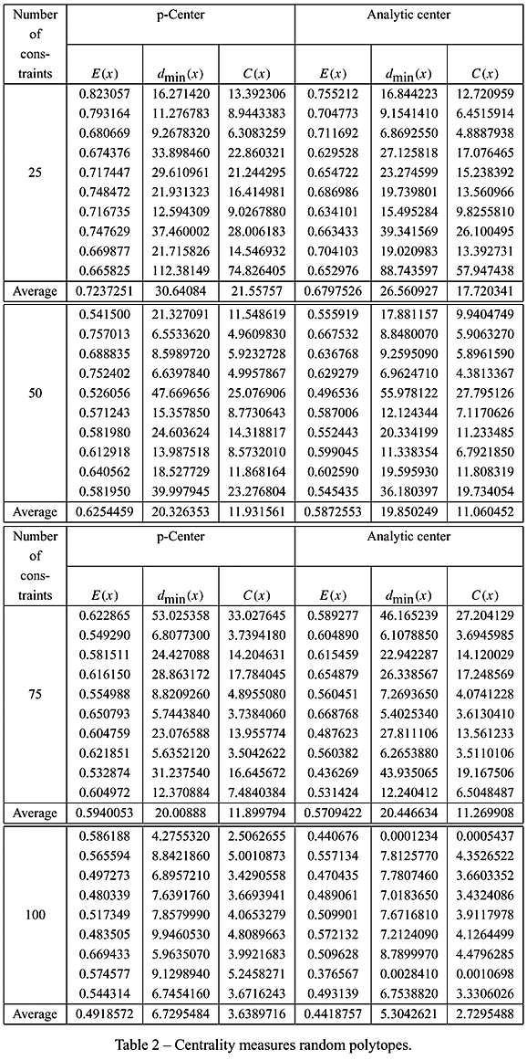
4.3 Randomly generated polytopes

We consider the problem of applying the projection method in randomly generated polytopes. Since special structure consistent with the class of real world problems being simulated is welcome, we generated the polytopes based on the work done by May [11]. We worked on polytopes with different dimensions and for each dimension we generated 10 different polytopes. The tables below present the measures E(x),d_min(x),C(x) and the average obtained for each dimension on each measure.

If we take in account the average for each dimension, we observed that the p-Center behaved better than the analytic center in all those problems.

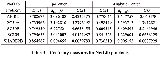
4.4 Netlib polytopes

Finally, we performed the computational experiences on some Netlib problems. We have transformed the problem to the dual format, i.e., all the constraints are of type " < ". In all the examples we have reached convergence. And, once more, the p-Center behaved well considering the measure used.

4.5 An application

Let us consider the problem of finding a feasible point in the region

W = {x Î Âⁿ : Ax < b, x > 0}

where we assume W is a full dimensional polytope. Also, we assume that

a_i = 1, i.e., b_i - is the real distance from x to the hyperplane {x Î Âⁿ : b_i - = 0}. The following algorithm will explain how the method works.

Algorithm: to find a feasible point in W

Initialization step :

S⁰ = {x Î Âⁿ : 0 < x < u}

where u = (M, M, ¼, M)^t, M Î Â is a large number

such that W Í S⁰.

Let x⁰ = *(1, 1, ¼, 1)^t.

Let k = 0.

The k^th iteration :

If x^k Î W then stop : we have reached a feasible point.

Otherwise :

There exist a k such that b_k - ^k > 0.

Let S^k+1 = S^k È{< ^k }.

Let x^k+1 be the center of S^k+1.

Let k = k + 1.

In the next section, we give an example to illustrate this procedure. We also apply the procedure to the same NetLib problems used in the previous section. The p-Center needs less cuts than the analytic center to get to a feasible point. We believe that this happens because the p-Center is more central than the analytic center.

4.5.1 An illustrative example

Let us consider the bidimensional polytope shown in the figures below as a shaded region. We define a square that contains the original polytope and its center as the initial point for the process. We use x₀ to denote the initial point and the symbol '*' is used to denote the center for each iteration. Figure (5) show that the analytic center used 4 cuts against 2 cuts for the p-Center.

4.5.2 NetLib problems

We solved some NetLib problems to verify the performance of the p-Center against the analytic center. Table (4) shows the outcomes for the feasibility problem applied to some NetLib problems.

As we can note, the p-Center needed less cuts than the analytic center to get to a feasible point. We believe this is the case because the p-Center is more central than the analytic center and, therefore, cuts a larger portion of the polytope.

4.6 Conclusions

The method described in this article has some nice properties as

• no changes are made to the original matrix: to compute the projections we need only the original data;

• it is less prone to accumulation errors: in each iteration, we use only the original data, therefore, there are no rounding errors from one iteration to the following iterations;

• it is easily implemented in a parallel environment: the projections are independent, we need only the actual iterate and then the projections can be done separately;

• it is less sensitive to redundant constraints: since the p-Center is geometrical.

Therefore, it can be applied in an environment of huge, sparse and unstructured matrices. And, to speed up the results a parallel implementation would be a must.

Based on our numerical experiments, the p-Center is more central than the analytic center. The performance of the p-Center was better than the analytic center if we consider our notion of centrality. Also, the p-Center behaved better for the feasibility problem applied to some NetLib problems. This brings us the belief that the p-Center is more central than the analytic center because the numerical experiences show it cuts a larger portion of the artificial polytope, pushing the centers towards the original polytope at a faster pace.

5 Acknowledgements

We are grateful to the two anonymous referees for their valuable remarks.

#538/01.

• [1] Bartle, R., The Elements of Real Analysis, second edition, John Wiley and Sons (1964).
• [2] Barnes, Earl and Moretti, Antonio C., A New Characterization of the Center of a Polytope, Computational and Applied Mathematics, 16(3) (1997), pp. 185-204.
• [3] Boggs, P., Domich, P., Donaldson, J. and Witzgall, C., Algorithmic Enhancements to the Method of Centers for Linear Programming Problems, ORSA Journal on Computing, 1(3) (1989), pp. 159-171.
• [4] Fenchel, W., Convex Cones, Sets, and Functions, report, Princeton University, N.J. (1953).
• [5] Freund, R., Projective Transformation for Interior Point Methods and a Superlinear Convergent Algorithm for the w-Center Problem, Mathematical Programming, 58 (1993), pp. 385-414.
• [6] Huard, P., Resolution of Mathematical Programming with Nonlinear Constraints by the Method of Centres, J. Abadie ed., Nonlinear Programming, North-Holland, (1967), 207-219.
• [7] Jarre, F., Sonnevend, G. and Stoer, J., An Implementation of the Method of Analytic Center, Lecture Notes in Control and Inform. Sci., Springer-Verlag 111 (1988), pp. 297-307.
• [8] John, F., Extreme problems with inequalities as subsidiary conditions, Studies and Essays , presented to Courant on the ocassion of his sixtieth birthday, Interscience Publishers, New York, (1948), pp. 187-204,
• [9] Kaiser, M.J., Morin, T.L. and Trafalis, T.B., Centers and Invariant Points of Convex Bodies, DIMACS Series in Discrete Mathematics and Theoretical Computer Science, 4 (1991), pp. 367-385.
• [10] Klee, V., Convexity, Proceedings of the Seventh Symposium in Pure Mathematics of The American Mathematical Society (1963).
• [11] May, Jerrold H. and Smith, Robert L., Random Polytopes: Their Definition, Generation and Aggregate Properties, Mathematical Programming, 24, pp. 39-54.
• [12] Renegar, J., A Polynomial-Time Algorithm, Based on Newton's Method, for Linear Programming, Mathematical Programming, 40 (1988), pp. 59-93.
• [13] Roos, C. and Vial, J.P., A Polynomial Method of Approximate Centers for Linear Programming, Mathematical Programming, 73 (1992), pp. 291-341.
• [14] Schrijver, A., Theory of Linear and Integer Programming, Wiley-Interscience series in discrete mathematics and optmization, (1986).

*

Supported by research grant 300198/93-0, CNPq-Brazil.

Publication Dates

• Publication in this collection
  19 July 2004
• Date of issue
  2003