Periodic boundary value problems for impulsive neutral differential equations with multi-deviation arguments

Periodic boundary value problems for impulsive neutral differential equations with multi-deviation arguments

Guobing Ye^I,*; Jianhua Shen^II; Jianli Li^III

^ICollege of Science, Hunan University of Technology, Zhuzhou Hunan 412008, PR, China

IICollege of Science, Hangzhou Normal University, Hangzhou Zhejiang 310036, PR, China

IIICollege of Mathematics and Computer Science, Hunan Normal University Changsha Hunan 410081, PR, China E-mails: [e-mail] / [e-mail] / [e-mail]

ABSTRACT

We develop the impulsive inequality and the classical lower and upper solutions, and establish the comparison principles. By using these results and the monotone iterative technique, we obtain the existence of solutions of periodic boundary value problems for a class of impulsive neutral differential equations with multi-deviation arguments. An example is given to demonstrate our main results.

Mathematical subject classification: Primary: 34A37; Secondary: 34k10.

Key words: Impulsive neutral differential equation, periodic boundary value, impulsive inequality, lower and upper solutions, monotone iterative technique, extremal solution.

1 Introduction

Impulsive differential equations have become more important in recent years in some mathematical models of real phenomena, especially in control, biological or medical domains (see, for example, [1-5]). As to periodic boundary value problems for impulsive differential equations, many authors have obtained excellent existence results; see, for instance, [7-11] for impulsive differential equations, [15-18] for impulsive neutral functional differential equations, [19] for abstract impulsive neutral functional differential equations. In [15-19], the characters of their neutral types are

respectively. In this paper, however, the character of its neutral type is (u(θ(t)))'. The character is different from the previous ones. Consider the following periodic boundary value problems for impulsive neutral differential equations with multi-deviation arguments of the form

where 0 = t₀ < t₁ < ... < t_p < t_p+1 = T; θ ∈ C¹(J,), θ is monotone increasing with 0 < θ(t) < t (t ∈ J),θ(0) = 0,θ(T) = T, and set θ(ζ_k) = t_k (k = 1,...,p),J₀ = J \{t₁,...,t_p}, J₁ = J \{ζ₁,...,ζ_p}; f: J×^q+1→ is continuous almost everywhere, and φ_i:J→ continuous with φ_i(J) ⊆ J (i = 1,...,q); and I_k ∈ C(,), Δu(t_k) = u-u(t_k). Denote by PC(X,Y), where X ⊂ ,Y ⊂ , the set of all functions u: X→Y which are piecewise continuous in X with points of discontinuity of the first kind at the points t_k ∈ X, i.e., there exist the limits u< ∞ and u = u(t_k) < ∞. PC¹(X,Y) denotes the set of all functions u ∈ PC(X,Y), that are continuously differentiate for t ∈ X, t ≠ t_k. Let Ω = PC([0,T],)∩PC¹([0,T],).

Definition. We say that the functions α,β ∈ Ω are lower and upper solutions of (1.1), respectively, if there exist M > 0 and 0 < L_k < 1 such that

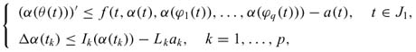
where

and

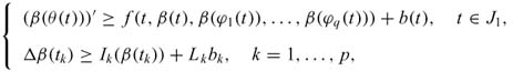
where

The definitions of classical lower and upper solutions make reference to the case α(0) < α(T) and β(0) > β(T).

2 Preliminaries

Lemma 1. Let s ∈ [0,T], c_k> 0, α_k,k = 1,...,p be constants, p,q ∈ PC(J,), x ∈ PC¹(J,) and θ be set by (1.1). If

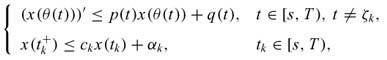
then for t ∈ [s,T],

This proof is similar to the one of [1], here we omit it.

Lemma 2. Let u ∈ Ω, M > 0, N_i > 0 (i = 1,...,q), 0 < L_k < 1 and θ be set by (1.1), such that

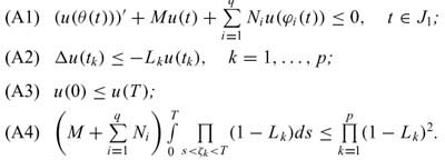
Then u< 0 on J.

Proof. By (A1) and (A2), we have

To prove u(t) < 0 on J, we shall consider the following two cases.

Case 1. u(t) > 0 for all t ∈ J. In this case, by (2.2) and (2.3) and the properties of θ, we get u'(t) < 0 on J₀ and u

< u(t_k), k = 1,...,p. Therefore u(t) is a non-increasing function on J. Then u(0) > u(T). Since u(0) < u(T), u(t) ≡ c on J (c is a non-negative constant), and u' = 0 on J₀. This and (A1) imply (M+N_i)c < 0. Then u ≡ 0 on J.

Case 2. There exists t^*∈ J such that u(t^*) > 0 and u(t) can take negative values in J. Let θ(ζ^*) = t^*. Again let = min{t ∈ J, inf_s∈J u(θ(s)) = u(θ(t)) = -λ, λ > 0}. Since (A3), ∈ [0,T). Without loss of generality, let ≠ ζ_k,, k = 1,...,p (If = ζ_k or , the proof is similar, here we omit.). In this case, we consider two subcases.

Subcase 1. u(T) > 0. From (2.1), we have

In view of (2.4), (2.3), and Lemma 1, we can get for t ∈ [,T],

Let t = T. Then we have

Since u(T) > 0, we get

which is contradictory to (A4).

Subcase 2. u(T) < 0. In this subcase, then < ζ^* or > ζ^*.

(i) < ζ^*. According to the same arguments as (2.5), we get

Multiplying both sides of the above inequality by Π_ζ*< ζ_k < T(1-L_k)(If ζ^* > ζ_p, this reduction is not needed.), we obtain

Since u(θ(ζ^*)) > 0, we have

which is contradictory to (A4).

(ii) > ζ^*. By (A3), we have u(0) < 0. This and the properties of θ imply 0 < ζ^*. According to the same arguments as (2.5), we get

Since u(θ(ζ^*)) > 0, we have

By (2.5) and (2.6), we obtain

Multiplying both sides of the above inequality by Π_ζ*< ζ_k < T(1-L_k) (If ζ^* > ζ_p, this reduction is not needed.), we get

which is contradictory to (A4).

Thus, in either case u < 0 on J. Therefore the proof of the Lemma iscomplete.

Lemma 3. Let u ∈ Ω, M > 0, N_i > 0 (i = 1,...,q), 0 < L_k < 1 and θ be set by (1.1), such that

(B1) (u(θ(t)))'+Mu(t)+N_iu(φ_i(t)) +[u(0)-u(T)] < 0, t ∈ J₁;

(B2) Δu(t_k) < -L_ku(t_k)-L_k×[u(0)-u(T)], k = 1,...,p;

(B3) u(0) > u(T).

Also assume that (A4) holds. Then u < 0 on J.

Proof. Set m(t) = u(t)+t/T·[u(0)-u(T)]. Clearly, m(0) = m(T). It follows that for t ∈ J₀,

and for t = t_k,

Δm(t_k) = Δu(t_k) < -L_ku(t_k)-L_k×t_k/T·[u(0)-u(T)] = -L_km(t_k).

By Lemma 2, we obtain m(t) < 0 on J, and so u(t) < 0 on J. Thus, we have completed the proof of the Lemma.

3 Existence for linear problem

In this section, we consider the linear problem of (1.1)

where σ(t) ∈ PC(J,), γ_k ∈ , k = 1,...,p, M > 0, N_i > 0 (i = 1,...,q), 0 < L_k < 1 and θ is set by (1.1). For α, β ∈ Ω, set [α,β] = {u|α(t) < u(t) < β(t),t ∈ J}.

Theorem 1. Suppose that there existα, β ∈ Ω such that

(C1) α < β on J;

(C2) (α(θ(t)))'+Mα(t)+N_iα(φ_i(t)) < σ(t)-a(t), t ∈ J₁

Δα(t_k) < -L_kα(t_k)+γ_k-a_k, k = 1,...,p;

(β(θ(t)))'+Mβ(t)+N_iβ(φ_i(t)) > σ(t)+b(t), t ∈ J₁

Δβ(t_k) > -L_kβ(t_k)+γ_k+b_k, k = 1,...,p,

where a(t),b(t),a_k,b_k are defined by (1.2)-(1.5). Also assume that (A4) holds. Then there exists a unique solution u for (3.1) with u ∈ [α,β].

Proof. We shall prove the Theorem in the following three steps.

Step 1. If u₁,u₂ are solutions of (3.1), set v₁ = u₁-u₂ and v₂ = u₂-u₁, then

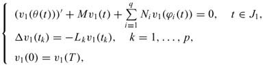
and

By Lemma 2, we obtain v₁ = u₁-u₂< 0 and v₂ = u₂-u₁< 0. Thus u₁ = u₂. Then there exists a unique solution u for (3.1).

Step 2. We prove that if ω,γ are classical lower and upper solutions, respectively, for (3.1) with ω < γ, then (3.1) has a solution u ∈ [ω, γ].

Let u(·,a) denote the unique solution of the following equation

Firstly, we show ω(0) < u(T,ω(0)) and γ(0) > u(T,γ(0)). Assume ω(0) > u(T,ω(0)). Let v(t) = ω(t)-u(t,ω(0)). Then the function v satisfies

By Lemma 2, we have v(t) < 0 on J. This implies v(T) = ω(T)-u(T,ω(0)) < 0. Thus ω(0) < ω(T) < u(T,ω(0)), which is contradictory to the above assumption. Then ω(0) < u(T,ω(0)). Similarly, we have γ(0) > u(T, γ(0)).

Next, we prove that there exists c ∈ [ω(0), γ(0)] such that u(0,c) = u(T,c). Now, we consider two cases.

Case 1. ω(0) = γ(0). In this case, we get ω(0) <u(T,γ(0)) <γ(0) = ω(0). Thus u(T,γ(0)) = ω(0). Then we choose c = ω(0), and so u = u(·,c) is a solution of (3.1).

Case 2. ω(0) < γ(0). In this case, we define the map F: [ω(0),γ(0)]→ by F(s) = s-u(T,s). Clearly F is continuous. Since F(ω(0)) < 0 < F(γ(0)), there must exist one point c ∈ [ω(0),γ(0)] such that F(c) = 0. Then u = u(·,c) is a solution of (3.1).

Finally, we claim u ∈ [ω,γ]. Let m₁(t) = ω(t)-u(t,c) and m₂(t) = u(t,c)-γ(t). It is evident that m₁,m₂∈ Ω, and

and

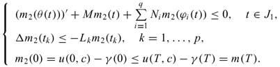
Using Lemma 2, we obtain m₁< 0 and m₂< 0 on J. Thus ω < u(·,c) < γ on J.

Step 3. We prove that (t),(t) are classical lower and upper solutions, respectively, for (3.1) with < , moreover [,] ⊆ [α,β], where

and

It is evident that α < and < β on J. Thus (0) = α(0) < (T) and (0) = β(0) > (T).

(i) If α(0) < α(T), then

and add to (0) < (T).

(ii) If α(0) > α(T), then

and add to (0) < (T).

Thus, in either case, is a classical lower solution for (3.1). The same arguments show that is a classical upper solution for (3.1).

Now, we consider the function m = -.

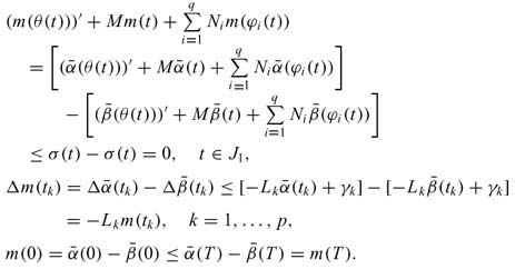
Using Lemma 2, we get m < 0 on J, i.e., < on J.

Thus, we have completed the proof of Theorem 1.

4 Existence for nonlinear problem

In this section, we establish the existence criteria for solutions of (1.1) by the lower and upper solutions and the monotone iterative technique.

Theorem 2. Suppose that there exist α,β ∈ Ω such that

(D1) α and β are lower and upper solutions for (1.1) with α < β;

(D2) f(t,x₂,y₁₂,...,y_q2)-f(t,x₁,y₁₁,...,y_q1) > -M(x₂-x₁)

N_i(y_i2-y_i1) for every t ∈ J₁, α < x₁< x₂< β,

α(φ_i(t)) <y_i1(φ_i(t)) <y_i2(φ_i(t)) <β(φ_i(t)) (i = 1,...,q);

(D3) I_k(x)-I_k(y) > -L_k(x-y) for α(t_k) < y(t_k) < x(t_k) < β(t_k),

k = 1,...,p.

Also assume that (A4) holds. Then there exist monotone sequence {_n(t)}, {_n(t)} with ₀ = ,₀ = , where ,are defined by (3.3) and (3.4), such that lim_n→∞

_n(t) = ψ(t) and lim_{n →∞}

_n(t) = ψ(t) uniformly hold on J,where ψ(t),ψ(t) are minimal and maximal solutions of (1.1), respectively.

Proof. We shall prove the Theorem in the following three steps.

Step 1. It is evident that α < and β < on J. Thus α(0) = (0) < (T) and (0) = β(0) > (T).

Let the function m = -, then m(0) = (0)-(0) < (T)-(T) = m(T). Next, we consider two cases.

Case 1. α(0) > α(T) and β(0) < β(T).

Firstly, by (D2), we get

Again, by (D3), we obtain

Finally, add to m(0) < m(T). Using Lemma 2, m(t) < 0 on J, i.e., < on J.

It follows that

Since α < < β, by (D2), we get

Then

From (D3), we get

Case 2. α(0) <α(T) and β(0) >β(T). In this case, it is trivial that we get (4.1) and (4.2).

Thus, in either case, is a classical lower solution. Similarly, is a classical upper solution. Moreover [,] ⊆ [α,β].

Step 2. For any η ∈ [,], we consider

Then, by Theorem 1, (4.3) has a unique solution u ∈ Ω.

Define operator A by u = Aη. Then A possesses the following properties:

(E1)

< A,> A;

(E2) Aη₁< Aη₂ for η₁,η₂∈ [,] with η₁< η₂.

Firstly, let m = -₁, where ₁ = A. Then we get

By Lemma 2, we have m(t) < 0 on J, i.e., < A. Similarly, we get > A.

Next, set v₁ = Aη₁ and v₂ = Aη₂, where η₁,η₂∈ [,] with η₁< η₂. Let m = v₁-v₂. By (D2), (D3) and (4.3), we get

By Lemma 2, we get m(t) < 0 on J, i.e., v₁< v₂ on J. Then Aη₁< Aη₂ for η₁, η₂ [, ] with η₁< η₂.

Step 3. Define the sequence {_n(t)}, {_n(t)} by _n+1 = A

_n, _n+1 = A_n, ₀ = , ₀ = . From (E1) and (E2), we get

Thus it is immediate to verify that

uniformly hold on J.

We consider the equation

and pass to the limit when n tends to ∞. Thus we obtain that ρ is a solution of (1.1). Analogously, ψ is also a solution of (1.1).

Finally, let u be any solution of (1.1) on [,]. Clearly ₀< u. Assume _n< u. We get that _n+1< u by considering the function m = u-_n+1 and using Lemma 3 again. Then by passing to the limit, we conclude ρ < u on J. Similarly, u < ψ on J. Then ρ(t), ψ(t) are minimal and maximal solutions of (1.1), respectively. Thus, we have completed the proof of Theorem 2.

5 An example

Now we consider the equation

Firstly, it is obvious that α = 0 is a classical lower solution for (5.1). Certainly α = 0 is a lower solution. Similarly β = 1 is an upper solution. Moreover α < β on J = [0,1]. Next,

for α < x₁< x₂< β, α

< y₁₁

< y₁₂

< β, α

< y₂₁

< y₂₂

< β, α

< y₃₁

< y₃₂

< β, where M = , N₁ = N₂ = N₃ = . Further, I₁(x)-I₁(y) = -x+y > -(x-y), for α

< y

< x

< β, where 0 < L₁ = < 1. Finally,

Then all the conditions of Theorem 2 are satisfied. Thus (5.1) has minimal and maximal solutions in [α,β].

In addition, we consider β₁(t) = , t ∈ [0,1]. Clearly β₁(0) < β₁(1), then b(t) =(++)+ and b₁ = . We still take M = , N₁ = N₂ = N₃ = . From

we have (β₁(t²))^'> - [β₁+β₁+β₁]+t+b(t). From 0 > -(×+)+×, we get Δβ₁

> I₁(β₁)+L₁b₁.

These show that β₁(t) is an upper solution for (5.1). Moreover α < β₁ on J. Similarly, we get the existence of monotone sequence that approximate the extremal solutions for (5.1) in [α,β₁].

Acknowledgements. The authors are very grateful to the referee for useful remarks and interesting comments.

Received: 02/X/09.

Accepted: 18/V/10.

• [1] D.D. Bainov and P.S. Simeonov, Impulsive Differential Equations: Periodic Solutions and Applications. Longman Scientific and Technical, Harlow (1993).
• [2] V. Lakshmikantham, D. Bainov and P. Simeonov, Theory of Impulsive Differential Equations. World Scientific, Singapore (1989).
• [3] A. Halanay and D. Wexler, Qualitative Theory of Impulse Systems. Editura Academic Republic Socialiste Romania, Bucuresti (1968).
• [4] A.M. Samoilenko and N.A. Perestyuk, Impulsive Differential Equations [M]. World Scientific, Singapore (1995).
• [5] X.L. Fu, B.Q. Yan and Y.S. Liu, Theory of impulsive differential system. Science Press, Beijing (2005).
• [6] R. Bellman, Mathematical Methods in Medicine. World Scientific, Singapore (1983).
• [7] M. Yao, A. Zhao and J. Yan, Periodic boundary value problems for second-order impulsive differential equations. Nonlinear Anal., 70 (2009), 262-273.
• [8] Y. Liu, Further results on periodic boundary value problems for nonlinear first order impulsive functional differential equations. J. Math. Anal. Appl., 327 (2007), 435-452.
• [9] J. Li and J. Shen, Periodic boundary value problems for delay differential equations with impulses. J. Comput. Appl. Math., 193 (2006), 563-573.
• [10] J. Li and J. Shen, Periodic boundary value problems for impulsive integro-differential equations of mixed type. J. Appl. Math. Comput., 183 (2006), 890-902.
• [11] J. Li and J. Shen, Periodic boundary value problems for impulsive differential-difference equations. Indian J. Pure Appl. Math., 35 (2004), 1265-1277.
• [12] Z. He and X. Ze, Monotone iterative technique for impulsive integro-differential equations with periodic boundary conditions. Comput. Math. Appl., 48 (2004), 73-84.
• [13] J. Shen, New maximum principles for first-order impulsive periodic boundary value problems. Appl. Math. Lett., 16 (2003), 105-112.
• [14] G. Song and X. Zhu, Extremal solutions of periodic boundary value problems for first order integro-differential equations of mixed type. J. Math. Anal. Appl., 300 (2004), 1-11.
• [15] Y.-K. Chang, A. Anguraj and M. Mallika Arjunan, Existence results for impulsive neutral functional differential equations with infinite delay. Nonlinear Analysis: Hybrid Systems, 2 (2008), 209-218.
• [16] A. Anguraj and K. Karthikeyan, Existence of solutions for impulsive neutral functional differential equations with nonlocal conditions. Nonlinear Anal., 70 (2009), 2717-2721.
• [17] C. Cuevas, E. Hernández and M. Rabelo, The existence of solutions for impulsive neutral functional differential equations. Comput. Math. Appl., 58 (2009), 744-757.
• [18] J.Y. Park, K. Balachandran and N. Annapoorani, Existence results for impulsive neutral functional integrodifferential equations with infinite delay. Nonlinear Anal., 71 (2009),3152-3162.
• [19] Eduardo Hernández Morales, Hernán R. Henríquez and Mark A. McKibben, Existence results for abstract impulsive second-order neutral functional differential equations. Nonlinear Anal., 70 (2009), 2736-2751.

*

The first author is supported by the NNSF of China (n. 10871062)

Publication Dates

• Publication in this collection
  22 Nov 2010
• Date of issue
  2010

History

• Received
  02 Oct 2009
• Accepted
  18 May 2010