A QUANTITATIVE EVALUATION OF DGPS PERFORMANCE IN THE POSITION AND PSEUDORANGE DOMAINS

Abstract:

This study compares in quantitative terms two methods of differential corrections to GPS positioning from the code-based pseudoranges. The differential method calculated from the coordinates (Latitude, Longitude and Altitude), called Position-Domain DGPS, has simple implementation and easy transmission by the correction vector. The second method, called Pseudorange-Domain DGPS has a more elaborate algorithm, focused on the pseudorange correction for each visible satellite, which consumes more processing time and increases the complexity in the transmission of the corrections. Notwithstanding a few variations from this DGPS techniques proposed, this work intends to verify in a numeric way the bias and precision offered by these two well-known methods in different devices and situations, to assess in which context each method would be more advantageous when one what to apply a simple DGPS correction; showing how much is the gain by way of bias the more elaborated method is. The results demonstrate that in favorable conditions, the Position-Domain offered an improvement of approximately 50% in positioning, 35% in dispersion, but without any significant bettering in altimetry or in the maximum values; wile the Pseudorange-Domain method showed 70% in positioning, 75% in precision, 60% for maximum values and numbers close to zero on average altimetry.

Keywords:
Differential GPS; Position-Domain DGPS Correction; Pseudorange-Domain DGPS Correction

1. Introduction

The techniques of GNSS (Global Navigation Satellite Systems) positioning can be divided into two main methods: absolute and relative positioning. Absolute positioning uses a single receiver to acquire and calculate its position, while relative positioning is based on the use of reference stations to support the user receiver. Generally, the absolute method is less accurate than the relative one and will not be studded in this article, but only be used as a reference for the quantitative analyses. The improvement when used the relative method occurs because there is a high correlation among ionospheric, tropospheric and satellite ephemeris errors between two stations. It can be especially true if the two stations are quite close, i.e., within a given area in which a certain homogeneity of the atmosphere can be considered (Seeber, 2003), that can be about 10 km.

Differential Global Positioning System (DGPS) is a relative technique to enhance the positioning using one or more reference stations, each equipped with a GPS receiver and sending corrections to user receiver (also called rover receiver). DGPS was originally developed to reduce the effects of the Selective Availability (SA), an intentional error imposed on the GPS in the absolute mode for civil users. SA was discontinued on May 1, 2000, but DGPS is still recommended for high-performance activities (Kaplan and Hegarty, 2006; Digglen, 2009; Seeber, 2003; Leick, 2015). Although the DGPS term is used in various relative positioning methods, historically the term has referred to the corrections made in the Carrier Code Positioning, also called standard point positioning (SPP) and in real-time (MONICO, 2008).

DGPS can be divided into two domains: Position Domain and Pseudorange (also called Measurement-Domain by some authors) Domain (Seeber, 2003; Kaplan and Hegarty, 2006; Sohn, 2017). Both are designed to provide differential corrections in real time (or near real-time). These corrections are calculated at the reference station and transmitted to users in formatted messages (usually Receiver Independent Exchange Format - RINEX data for post-processing/near real-time applications and Radio Technical Commission for Maritime Services - RTCM data for real-time applications) (Seeber, 2003). Although those methods are wheel known and widely divulgated in the literature, they always have a qualitative approach, where the pros and cons involved the two methods are discussed, but there is a gap in the literature about the quantitative approach, or how much a method is more accurate than the other, which makes the choice of one of the two methods difficult when one wants to make his election based in a weighting distribution between enhance and facility.

GPS receivers are produced by different receiver manufacturers with different technologies, components and algorithms, thereby producing different levels of precision and bias in the positioning. So, using different models of receivers, this research aims to compare in quantitative terms, the improvement of positioning obtained from the corrections calculated by the two methods to facilitate the choice of when a more accurate method is better in despite of an increased cost in the processing of information. Notwithstanding a few variations from the initial DGPS technique was proposed (Landau et al, 2009; Park et al, 2013 and Sohn et al 2017), here only the two well-known methods will be described and availed. Here it is appropriate to make it clear that in this work it was used a simulated DGPS, in other words, there was no transmission of corrections via radio link.

2.DGPS Fundamentals

If it is necessary to determine a position in real-time using only one GPS receiver, the recommendation is to use the code pseudoranges. This method, however, has some inherent errors deriving from the clocks of satellites, the satellites ephemeris parameters, atmospheric propagation, multipath and receiver noise (Monteiro, Moore and Hill, 2005; Kaplan and Hegarty, 2006). The DGPS technique was originally proposed to remove or at least to reduce the autonomous positioning errors (Seeber, 2003; Leick, 2015). This is based on the premise of a high correlation of errors between two separate GPS receivers from a reasonable distance (in Monteiro et al. 2005, the authors present an estimated error growth of 0.22 m per 100 km). The technique uses a Reference Station (RS) at a known location to calculate and send corrections to user receiver. The methods to calculate the corrections can be divided into two types: Position-Domain Correction and Pseudorange-Domain Correction.

2.1 Position-Domain DGPS Correction

Position-Domain DGPS Correction is the technique in which the position of a Reference Station is well-know a priori, and it is compared with the calculated position obtained from satellites. A vector of differences between these positions coordinates (latitude, longitude and geodetic altitude) is calculated according to the Equation 1:

$∆{\stackrel{⃑}{p}}_{RS}={\stackrel{⃑}{p}}_{RSfixed}-{\stackrel{⃑}{p}}_{RS}$ (1)

where $\mathrm{\Delta }{\stackrel{⃑}{p}}_{RS}$ is the correction vector (∆x, ∆y, ∆z or ∆φ, ∆λ, ∆h), ${\stackrel{⃑}{p}}_{RSfixed}$ are the coordinates from Reference Station and ${\stackrel{⃑}{p}}_{RS}$ is the calculated coordinates of Reference Station from signals of satellites. The vector calculated is transmitted and used to correct the position of a rover receiver (Figure 1). In most situations, the coordinate differences between the reference station and the rover receiver represent the most common errors in the positioning solution for a given moment.

Figure 1:
Position-Domain DGPS.

After receiving the correction vectors sent by the Reference Station, the rover applies the errors mitigation in its own solution (Equation 2), obtaining an improved positioning solution (Park et al., 2013):

${\stackrel{⃑}{p}}_{DGPS}={\stackrel{⃑}{p}}_{rover}+∆{\stackrel{⃑}{p}}_{RS}$ (2)

where ${\stackrel{⃑}{p}}_{DGPS}$ is the rover corrected solution, ${\stackrel{⃑}{p}}_{rover}$ is the rover estimated coordinates, and Δ p RS is the correction vector sent by Reference Station.

This technique has two major needs to be efficient (Kaplan and Hegarty, 2006): firstly, all receivers need to make pseudorange measurements of the same set of satellites to ensure the treatments of same type of errors. This can be made by a combination between Reference Station and rover receivers, or the Reference Station can send all possible combinations of the visible satellites. Secondly, all receivers need to employ the same techniques (algorithms, filters, etc.).

2.2 Pseudorange-Domain DGPS Correction

The Pseudorange-Domain DGPS (or Measurement-Domain DGPS) method consists of determining and applying the corrections to pseudoranges for each visible satellite before calculating the position (Seeber, 2003; Kaplan and Hegarty, 2006; Park et al., 2013). In principle, it is a more effective method and more widely used than the Position-Domain Correction. Figure 2 shows a diagram of the method.

Figure 2:
Pseudorange Domain DGPS.

Pseudorange is the distance between a specific satellite and a receiver antenna at the time of the code emission and reception (Park et al., 2013). Because it is a noisy estimate, it is also called “pseudo” range. It can simply be expressed by the mathematical model of Equation 3 (Seeber, 2003; Verhagen, 2005):

Where:

$P{R}_r^s=R_r^s+c\left(d{t}_r-d{t}_s\right)+I_r^s+T_r^s+{\delta }_{r.orbit}^s+{\delta }_{r.multipath}^s+\epsilon$ (3)

$P{R}_r^s$ is the pseudorange between the antenna of a satellite s_i (at the instant of transmission) and receiver r (at the instant of reception);

$R_r^s$ is the geometric distance between the antenna of satellite s_i at the instant of transmission, and receiver r at the instant of reception;

c is speed of light in vacuum;

dt_r is the receiver clock offset at reception instant;

dt_s is the satellite clock offset at transmission instant;

$I_r^s+T_r^s$ refer respectively to the ionospheric and tropospheric delays;

${\delta }_{r.orbit}^s+{\delta }_{r.multipath}^s$ describe the orbital and multipath errors; and

Ɛ refers to other effects not modeled.

The geometric distance is the true distance between two points. If the satellite and the receiver coordinates are known in the Earth Centered, Earth Fixed (ECEF) system, the geometric distance between these two points can be calculated using Equation 4:

$R_r^s=\sqrt{{(X_s-X_r)}^2+{(Y_s-Y_r)}^2+{(Z_s-Z_r)}^2}$ (4)

where (X_s , Y_s , Z_s ) are the satellites coordinates, (X_r , Y_r , Z_r )are the receiver coordinates.

From the pseudorange for each satellite, it is calculated the Pseudo Range Correction (PRC) at a reference time t₀ is given by Equation 5 (Hofmann-Wellenhof, Lichtenegger and Wasle, 2007):

${PRC}_s\left(t_0\right)={PR}_r^s\left(t_0\right)-R_r^s-c({dt}_r-{dt}_s)$ (5)

and the components of this expression have already been defined above.

Over time, there is a variation in the corrections, which occurs in an approximately linear way. Thus, the differential correction in the pseudorange accumulates, by the experience, an error of approximately 1.00 m every 10 s (Hofmann-Wellenhof, Lichtenegger and Wasle, 2007). It is hence necessary to calculate the rate of update of this correction. Therefore, in case a time interval value between corrections is necessary so that the result is not affected by this variation, not only Pseudo Range Correction is used, but also Range Rate Corrections (RRC) in time. The RRC is expressed in Equation 6:

$RRC\left(t_0\right)=\frac{PRC\left(t\right)-\left(PRC\right(t_0)}{(t-t_0)}$ (6)

where t₀ is the reference epoch, t is the epoch in which the PRC is intended and t-t₀ is the time interval that can be regarded as the age of correction, also called latency.

A new updated correction is produced for a given time t, which is expressed in Equation 7:

$PRC\left(t_i\right)=PRC\left(t_0\right)+RRC\left(t_0\right)x(t_i-t_0)$ (7)

Thus, the correction updated in time must be added to the pseudorange obtained from the rover receiver.

3. Experiments

This research compares bias and precision between the two DGPS methods previously cited. The tern bias is here used as stated by Monico (2009) and refers to systematics errors, wile precision indicates the spread or dispersion. For testing, two antennas were used as Reference Stations: both were installed at two points with well-known coordinate and positioned in open-sky, i.e. without obstructions or interference with the horizon line, thus, with a good reception of signals transmitted from almost all the satellites that could be visible.

The first antenna used has the name “Escola Politécnica da USP”, with id = “POLI” and International Code “41630M001”. This antenna is in the city of São Paulo, Brazil, and it is part of the Brazilian Network for Continuous Monitoring (in Portuguese Rede Brasileira de Monitoramento Contínuo - RBMC). This base has a GNSS choke ring antenna (TRM 59800.00) and a TRIMBLE receiver NETR8 model. The second antenna (from the same manufacturer and model of first antenna) was placed on top of the Civil Engineering Building of Polytechnic School of University of São Paulo, with 155.08 meters away from the first antenna and 1.83 meter lower in altitude. This proximity together with a very clear sky ensures a good scenario for the corrections, as almost always the two receivers will be tracking the same satellite set at the same time, ensuring for that moment the best correlation and PDOD which was always between 1.2 and 1.8 for the two stations.

From the second antenna four campaigns were carried out with four different types of equipments, just to check if all devices show the same performance. They are:

Novatel L1 receiver: which collected data from 08:55:45 h December 21, 2015 to 10:48:00 h December 23, 2015, with a collect rate of 15 seconds.

Topcon Hiper (L1/L2) receiver: that collected data from 16:21:30 h December 14, 2015 to 16:59:00 h December 16, 2015, with a collect rate of 15 seconds, too.

Magellan ProMark 3 (L1) receiver: that collected data from 17:19:30 h April 14, 2016 to 10:47:45 h April 16, 2016, with a collect rate of 5 seconds.

U-blox Lea-6T (L1) receiver: that collected data from 18:00:00 h April 14, 2016 to 13:41:00 h of April 20, 2016, with collect rate of 5 seconds.

Despite measuring the carrier phase differences among other observables, the receivers also measure the pseudorange from the code, the object of this study. All devices generated RINEX files that were analyzed and edited in the freeware software TEQC, developed and maintained by UNAVCO (Estey and Wier, 2014), and the result was a consistent file with only the pseudorange observable. The program was implemented with the option of excluding all observables other than C1 (GURTNER, 2001), i.e. in the RINEX file, just code pseudoranges obtained by CA on L1 frequency remain. To be compared with the knows positions, the coordinates of the stations were processed by the single-point positioning, conducted by the RTKLIB Software, an open source program package for standard and precise positioning with GNSS (Takasu and Yasuda, 2013).As the rover station coordinates are known with millimetric precision, the bias evaluation was performed by comparing the calculated coordinates with these known coordinates. This was done for the coordinates obtained by single positioning coordinates and for those obtained by both methods of differential correction. In turn, the precision was assessed by the standard deviation of each set of measures.

For calculating the DGPS in the Position Domain, the corrected coordinates were determined by the simple addition of the correction vector. Whereas, for the corrections in the Pseudorange Domain, a C programming language software was developed for the present work: from two RINEX files, it calculates the point position coordinates, and using the algorithms described in item 2.1, it provides the epoch to epoch coordinates correction.

As stated earlier, the correction vector from the positions (Position Domain) is intrinsically related to the fact that both the reference station and the rover station track the same set of satellites. Thus, another program was created, also in C programming language, which emulates an urban canyon by calculating satellites azimuths and elevations for a given position and generating a mask that simulates obstructions and eliminates the satellites that would not be available for tracking. This program generated a modified new RINEX file, which was also submitted to the same tests described above.

3.1 DGPS without satellite cut

Three types of positioning are compared in this step: 1) Single Point Positioning, 2) DGPS in Position Domain and 3) DGPS in Pseudorange Domain. All the processed information was obtained from the RINEX files.

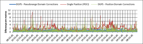
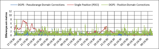
The position error can be estimated by the plane distance between the Rover Station (with known coordinates) and the point defined by the GPS estimated coordinates. The behavior of this value (variable over time), for each receiver, can be seen in Figures 3 to 6.

Figure 3:
2D Error or difference in positioning from 16:21:30 h December 14, 2015 to 16:59:00 h December 16, 2015 - Hiper.

Figure 4:
2D Error or difference in positioning from 08:55:45 h December 21, 2015 to 10:48:00 h December 23, 2015 - Novatel.

Figure 5:
2D Error or difference in positioning from 17:19:30 h April 14, 2016 to 10:47:45 h April 16, 2016 - ProMark 3.

Figure 6:
2D Error or difference in positioning from 18:00:00 h April 14, 2016 to 13:41:00 h of April 20, 2016 - U-blox LEA 6T.

These graphics show the horizontal distances (that are associated to the bias) which is obtained with the single position minus known position, taken as correct; in the vertical axis, varying over universal time - UT (on the horizontal axis). In red is the behavior obtained by absolute positioning (single receiver), which shows quite a noisy behavior and subject to atmospheric interferences, such as greater dispersion of the TEC (Total Electron Content) at night when can be seen the majors discrepancies in the graphics, due to the ionospheric effects (Fonseca Júnior, 2002; Dey et al, 2016).

The green line shows the errors when the correction in the Position Domain is chosen, a solution that generally presents improvements with respect to the solution of single positioning (in red), and apparently fixes (mitigates) the atmospheric effects; this was expected since the distance between the base station and the rover station is short. Still it shows to be quite noisy (sharp peaks) and, in addition, at various times a worsening in positioning is noticed rather than an improvement (green line positioned above the red). This situation becomes more common the cheaper the receiver is, probably due to the lower quality of its electronic components, as for example in the quality of the oscillator (clock), which influences the correlation process, responsible for obtaining the pseudoranges.

The performance of the Pseudorange Domain corrections is shown in blue. It can be seen a more homogeneous behavior in comparison with the others (smaller fluctuations and peaks), regardless of the model of the equipment, with a smaller amplitude range and with few points outside of a defined range (for example, 2 m).

These graphs show a similar and cyclic behavior for the various receivers. For the autonomous positioning (red line), there are daily peaks around the 20:00 UT, which corresponds to the moments of usually occurs the greatest ionospheric effects, how can be seen in Fonseca Júnior (2002). This is mitigated with the correction in the Position Domain (green line) and practically removed with the correction in the Pseudorange Domain.

Tables 1 to 4 present the statistical summary of the values obtained for each of the techniques applied, not only for the horizontal distance, but also differences for each coordinate separately in columns dLat, dLong, dAlt and RMS, displaying, respectively, the differences in meters in Latitude, Longitude, Altitude and horizontal distance between the calculated and known values of the Rover Station. The column improvement (Improv.) exhibits in percentage how much the bias was improved, as is the case of the distance (RMS), when comparing this value calculated by the Single Point Positioning and that obtained by the DGPS method, which is exposed in equation 8. Negative values indicate a worsening in the process.

$Improv=\frac{\left({RMS}_{SinglePositioning}-{RMS}_{DGPS}\right)}{{RMS}_{SinglePositioning}}\times 100$ (8)

Table 1:
Statistical summary of the data obtained by the receiver Hiper.

Hiper	Single Positioning				DGPS Position Domain					DGPS Pseudorange Domain
	dLat	dLon	dAlt	RMS	dLat	dLon	dAlt	RMS	Improv.	dLat	dLong	dAlt	RMS	Improv.
Mean (m)	1.25	-0.96	1.82	2.21	0.25	-0.04	1.68	1.08	51%	0.13	-0.06	0.13	0.74	67%
Std-Deviation (m)	1.78	1.32	2.74	1.59	1.11	0.92	3.23	0.98	38%	0.62	0.55	1.31	0.41	74%
Range (m)	10.40	7.95	20.87	8.17	12.78	14.56	53.22	8.39	-3%	7.01	4.60	23.43	3.75	54%
Minimum (m)	-3.11	-5.86	-8.22	0.01	-5.80	-7.38	-12.6	0.01	-52%	-3.27	-2.38	-6.01	0.00	53%
Maximum (m)	7.29	2.09	12.65	8.18	6.99	7.17	40.61	8.40	-3%	3.74	2.22	17.41	3.75	54%
Count	11670				11670					11670

Table 2:
Statistical summary of the data obtained by the receiver Novatel.

NOVATEL	Single Positioning				DGPS Position Domain					DGPS Pseudorange Domain
	dLat	dLon	dAlt	RMS	dLat	dLon	dAlt	RMS	Improv.	dLat	dLong	dAlt	RMS	Improv.
Mean (m)	1.04	-0.63	-1.52	2.01	0.14	-0.23	0.20	0.81	60%	0.12	-0.03	0.14	0.53	74%
Std-Deviation (m)	1.52	1.25	3.65	1.14	0.88	0.79	2.70	0.90	21%	0.44	0.40	0.91	0.29	74%
Range (m)	13.50	12.43	32.21	10.99	13.43	9.99	42.98	9.52	13%	4.27	3.38	8.95	2.42	78%
Minimum (m)	-4.89	-8.30	-21.2	0.00	-5.65	-6.90	-18.8	0.00	32%	-2.18	-1.70	-4.54	0.00	63%
Maximum (m)	8.60	4.13	11.02	11.00	7.78	3.10	24.14	9.52	13%	2.09	1.68	4.41	2.42	78%
Count	11792				11792					11792

Table 3:
Statistical summary of the data obtained by the receiver ProMark 3.

ProMark3	Single Positioning				DGPS Position Domain					DGPS Pseudorange Domain
	dLat	dLon	dAlt	RMS	dLat	dLon	dAlt	RMS	Improv.	dLat	dLong	dAlt	RMS	Improv.
Mean (m)	1.13	-0.60	-1.30	1.61	0.16	-0.11	2.17	0.98	39%	0.15	-0.06	0.05	0.57	65%
Std-Deviation (m)	1.51	0.99	2.60	1.52	1.03	0.77	2.81	0.85	44%	0.47	0.43	1.03	0.33	78%
Range (m)	8.17	6.16	16.30	7.58	12.20	7.41	22.35	8.09	-7%	4.78	5.21	14.78	3.49	54%
Minimum (m)	-1.60	-4.60	-8.10	0.01	-4.11	-3.86	-5.63	0.01	0.5%	-1.80	-2.00	-5.23	0.01	22%
Maximum (m)	6.57	1.56	8.20	7.59	8.09	3.55	16.72	8.10	-7%	2.98	3.22	9.55	3.50	54%
Count	9839				9839					9839

Table 4:
Statistical summary of the data obtained by the receiver U-blox LEA 6T.

Ublox	Single Positioning				DGPS Position Domain					DGPS Pseudorange Domain
	dLat	dLon	dAlt	RMS	dLat	dLon	dAlt	RMS	Improv.	dLat	dLong	dAlt	RMS	Improv.
Mean (m)	1.50	-0.81	-3.53	2.23	0.80	-0.33	0.48	1.35	39%	0.14	0.09	0.00	0.75	66%
Std-Deviation (m)	1.77	1.24	3.89	1.61	1.05	0.98	3.47	0.99	38%	0.61	0.57	1.26	0.42	74%
Range (m)	18.03	10.70	40.58	12.25	15.19	10.98	52.45	10.20	17%	8.58	7.38	15.43	5.03	59%
Minimum (m)	-6.38	-6.97	-30.1	0.01	-5.01	-6.51	-33.0	0.01	-2%	-4.06	-3.78	-7.15	0.00	66%
Maximum (m)	11.66	3.73	10.50	12.27	10.18	4.47	19.44	10.21	17%	4.51	3.61	8.28	5.04	59%
Count	32323				32323					32323

In these tables, the value of the average error (mean) and its standard deviation can be compared for each type of equipment in the three methods; the RMS and Improv. columns summarize the resulting improvement. The range, in turn, is a measure of the fluctuation or amplitude of the results. Before making a final assessment, another way to evaluate the results in graphic form is presented.

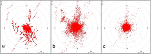
Another way to illustrate the behavior and trends of positioning is using the scatter plot, which consists in plotting or drawing points through its coordinates (dLat and dLong), epoch by epoch, around a point source, which represents the Rover Station known coordinates. Figure 7 shows the horizontal alignment error of the surveys performed by the ProMark3 receiver in meters and using the same scale for the three cases. The graphs of the other receiver features present the same pattern as for the dispersal and therefore will not be represented.

Figure. 7:
Errors dispersions for the rover station - a) Single Positioning; b) DGPS in Position Domain; c) DGPS in Pseudorange Domain.

By analyzing the graphs, the differential correction in the Position Domain is verified to provide a clear improvement in the bias of the coordinates, which is proven by the numbers in Table 3, where an improvement of 39% on the value of the horizontal distance or in bias average is observed; it decreases from 1.61 m to 0.98 m. There is also an improvement of 44%, in this variable precision, which decreases from 1.52 m to 0.85 m. There are some occasional fluctuations, however, which determine a larger range (8.09 versus 7.58), reflecting the value of -7%. However, in altitude there is degradation in the quality in all cases.

The points plotted from the DGPS Pseudorange Domain correction proved to be better, with most of values within the range of 2.00 m, a fact associated with a better bias and lower standard deviation. The values of Table 1 also show that the bias and precision obtained via this method are closer to the values taken as true, in addition to improving the values of altimetry in all types of equipment tested.

Regarding bias, the mean values of the differences in Latitude and Longitude (dLat and dLon) listed in the Tables from 1 to 4 cannot fail to be noted. This approach is due to the large number of samples and only has some representative meaning if the purpose of positioning is in the static mode, since in the kinematic mode, the averages of the coordinates do not make sense; cause each point positioning will be taken in a different place.

One of the ways to measure where the mean tendency is converging to is by the progressive average. Progressive average is calculated for each time, using the help of simple arithmetic average of the cumulative average. Unlike the moving average, all values are used without discarding information over time. The graphs presented in Figure 8 show the trend of convergence when used the ProMark 3 receiver during the test for a period of 24 hours; this tendency was obtained by the progressive and moving averages calculated from the Latitudes and Longitudes differences obtained from the tracking and the known rover station coordinates.

Figure 8:
Positioning tendency from the Progressive Average and the moving average - ProMark 3.

The single positioning is show in blue lines, the DGPS in the Position Domain in green and the DGPS with Pseudorange Domain in red; the continuous line demonstrates progressive average and the dotted one, a 1-hour moving average period.

The solid line shows an improvement in the first hour of data collection followed by a worsening in the second and third hours. This behavior could mislead us to believe that the best results could be obtained with 1 hour of tracking. Yet the moving average (1-hour period) demonstrates that those values vary throughout the day, the time of year and the solar cycle, in the same way as noticed in previous graphs.

Another result from this graph is that the autonomous positioning tends to stabilize after 8:00 hours of tracking, the DGPS in the Position Domain between 4:00 and 5:00 hours and DGPS in the Pseudorange Domain around 3:00 hours.

3.2 DGPS with satellite cut

As above, the single positioning generally occurs in places where the horizon is blocked by buildings, trees or hills; therefore, for simulations, a software written in C-language was developed to simulate the cut of some satellites in this situation, using the same data tracked and used previously. This cut is made by a mask that simulates obstructions in certain regions of space, with intervals of azimuth and vertical cutting angles.

From the coordinates of the satellites and the known position of the Rover Station, the azimuth and elevation were calculated for each visible satellite at any given instant, eliminating those that were within the range defined by the cutting mask, generating a new RINEX file.

Initially, a clipping mask was tested between the azimuths from 30° to 150° and from 210° to 330°, with an elevation of 60°. The result was unsatisfactory, since there were a few epochs with less than four satellites, the minimum quantity to obtain a point positioning solution. Thus, maintaining the ranges in azimuth, a cutting angle of 30° in elevation was adopted for the new mask. This value simulates an urban canyon with a street of two-story houses on each side.

Hence, the survey from the four receivers previously studied underwent simulated obstructions with this mask, generating new data that were processed by following the same methodology as in previous section “DGPS without satellite cut”.

As expected, the results showed deterioration in the quality of the positioning, since there was a decrease in the number of tracked satellites and, consequently, an increase in Position (3D) Dilution of Precision (PDOP)and other Dilution of Precision (DOP)s.

Yet, despite some points which are out of place, with disparate values, they do not result in a trend in the results (average offset), or major modifications in the standard deviation, probably by size, still great, of the sample. These “outliers” do not appear on the charts, as shown in Fig. 10; they were cut because their magnitude would greatly decrease the scale, which would hinder the visualization of information.

Since the behavior of the degradation is similar in all the equipment used, then just the graphs obtained by ProMark 3 data (Figure 9) depict the behavior of the absolute deviation in position, and can be compared with Fig. 5 (same receiver, without satellite cut). It may be immediately noted that the best method (DGPS Pseudorange Domain correction, in blue) presents some peaks of great error magnitude (about 10 m).

Figure 9:
Absolute positioning deviation with mask - ProMark 3.

Figure 10 displays the scatter of the single positioning, DGPS (Position Domain) and DGPS (Pseudorange Domain).

Figure 10:
Errors dispersions for the rover station with mask - a) Single positioning; b) DGPS in Positioning Domain; c) DGPS in Pseudorange Domain

Tables 5 to 8 show the statistical summary of the new data for each of the techniques applied to the four receivers.

The DGPS in the Position Domain was calculated by resorting to the same vectors previously used, i.e. with a different set of satellites to the base and to the rover; to the base there were, on average, 11 satellites visible in the sky; after cutting, there were only 6 satellites, on average.

Table 5:
Statistical summary of the data obtained by the receiver Hiper - with mask.

Hiper	Single Positioning				DGPS Position Domain					DGPS Pseudorange Domain
	dLat	dLon	dAlt	RMS	dLat	dLon	dAlt	RMS	Improv.	dLat	dLong	dAlt	RMS	Improv.
Mean (m)	0.71	-0.53	2.45	2.05	-0.30	0.40	2.31	1.82	11%	0.12	-0.06	0.02	0.92	55%
Std-Deviation (m)	2.15	1.41	9.82	1.79	1.94	1.60	10.19	1.81	-1%	1.05	0.71	4.12	0.89	50%
Range (m)	65.45	42.66	415.84	53.47	63.87	45.67	414.19	53.06	1%	39.44	15.76	185.36	20.44	62%
Minimum (m)	-51.7	-13.8	-368.9	0.02	-51.7	-11.9	-372.3	0.01	69%	-19.0	-6.05	-59.17	0.01	45%
Maximum (m)	13.77	28.85	46.93	53.49	12.15	33.82	41.94	53.06	1%	20.42	9.71	126.19	20.45	62%
Count	11636				11636					11636

Table 6:
Statistical summary of the data obtained by the receiver Novatel - with mask.

NOVATEL	Single Positioning				DGPS Position Domain					DGPS Pseudorange Domain
	dLat	dLon	dAlt	RMS	dLat	dLon	dAlt	RMS	Improv.	dLat	dLong	dAlt	RMS	Improv.
Mean (m)	0.53	-0.21	-0.46	1.71	-0.37	0.21	1.26	1.58	7%	0.10	-0.01	0.02	0.74	57%
Std-Deviation (m)	1.71	1.27	6.94	1.38	1.61	1.27	6.80	1.37	1%	0.91	0.57	3.82	0.79	43%
Range (m)	23.03	17.89	153.15	16.16	27.34	19.19	154.59	16.84	-4%	28.43	20.75	250.98	18.26	-13%
Minimum (m)	-15.0	-9.02	-112.1	0.01	-16.7	-7.22	-112.2	0.00	48%	-13.7	-10.78	-142.7	0.00	58%
Maximum (m)	8.03	8.87	41.07	16.17	10.67	11.96	42.41	16.84	-4%	14.74	9.97	108.30	18.26	-13%
Count	11892				11892					11892

Table 7:
Statistical summary of the data obtained by the receiver ProMark 3 - with mask.

ProMark3	Single Positioning				DGPS Position Domain					DGPS Pseudorange Domain
	dLat	dLon	dAlt	RMS	dLat	dLon	dAlt	RMS	Improv.	dLat	dLong	dAlt	RMS	Improv.
Mean (m)	0.85	-0.27	0.82	2.20	-0.12	0.22	4.27	1.93	12%	0.11	-0.08	0.01	0.72	67%
Std-Deviation (m)	3.24	2.15	11.08	3.33	3.22	2.15	10.83	3.36	-1%	0.77	0.62	3.33	0.70	79%
Range (m)	166.67	106.94	436.59	102.64	167.11	107.20	434.83	102.04	1%	24.27	15.43	132.67	17.93	83%
Minimum (m)	-85.89	-56.22	-229.7	0.02	-85.07	-56.37	-227.6	0.02	13%	-15.2	-9.47	-65.27	0.00	80%
Maximum (m)	80.78	50.72	206.85	102.66	82.04	50.83	207.18	102.05	1%	9.05	5.96	67.40	17.93	83%
Count	9941				9941					9941

Table 8:
Statistical summary of the data obtained by the receiver Ublox - with mask.

Ublox	Single Positioning				DGPS Position Domain					DGPS Pseudorange Domain
	dLat	dLon	dAlt	RMS	dLat	dLon	dAlt	RMS	Improv.	dLat	dLong	dAlt	RMS	Improv.
Mean (m)	0.70	-0.43	-0.95	2.01	0.02	0.03	3.06	1.84	8%	0.17	0.26	0.11	1.06	47%
Std-Deviation (m)	2.02	1.70	9.97	1.89	1.92	1.72	9.79	1.81	4%	0.96	0.90	4.49	0.84	56%
Range (m)	34.73	42.74	337.82	26.83	37.35	42.51	338.52	25.93	3%	24.96	20.65	252.50	13.28	51%
Minimum (m)	-19.7	-26.8	-160.1	0.01	-21.7	-25.8	-158.0	0.01	-40%	-13.3	-10.48	-121.8	0.00	93%
Maximum (m)	15.00	15.98	177.72	26.84	15.64	16.67	180.52	25.94	3%	11.68	10.17	130.75	13.28	51%
Count	32518				32518					32518

The Figure 10 shows an inconstant behavior for this method under these circumstances, improving the positioning in some moments and worsening in others. From Table 7, the DGPS, in the Position Domain, presents an average improvement of 12% in the plane position, or 0.27 m in 2.20 m, with a significant worsening occurring in altitude (1.93, when it was 0.82). It also points to an improvement in bias (dLat and dLong averages) and maintenance of precision (standard deviation).

However, the DGPS Pseudorange Domain proved to be more constant, by using only the correction for the same set of satellites, without including a new source of errors such as the PDOP difference of the two stations. In Fig. 8, in blue, the Pseudorange Domain appears more regularly decreasing the errors in a more significant way, although in a few cases it presents greater values than those from single positioning.

In statistical terms, it introduces improvements in all aspects, both in bias with 67%, and in precision (standard deviation) that reaches 79%. The correction in altitude is 99%, bringing the altimetry average error from 0.82 m to 0.01 m with standard deviation of 3.33 m, when used the ProMark 3, and with similar results to the other receivers.

In all the cases and for all the receivers, the “Range” values (third line in the tables) increase compared with the values without satellite cut. It is very nonstandard: it grew significantly, in some cases reaching 300, 400 m or more. That is because the sample was contaminated with very poor point solutions in the coordinate calculation with very few satellites, just four, sometimes, and with a very bad geometry.

4. Discussion and conclusion

The scenario created for the tests produced a highly favorable situation for applying differential correction methods, notably: the proximity of the two bases, the placement of the antennas with free horizon and use of choke ring antennas with ground plane which allow minimizing multipaths.

Under these conditions and for these types of equipment, the single positioning or autonomous positioning reveal an expected error of 2.00 m in planimetry and a standard deviation (measure of precision) of ± 1.50 m, and may also present maximum error values in the order of 12.00 m; in average values. In altimetry, the average error (measure of bias) was -1.10 m with a standard deviation of 3.20 m.

The DGPS in the Position Domain offered an improvement of approximately 50% in positioning and 35% in precision, but without improvement or in some cases with some worsening in altimetry and with the same results in the maximum values. The Pseudorange Domain method showed 70% improvement in bias, 75% in precision and 60% for maximum values and numbers close to zero on average altitudes.

With the mask insertion, emulating a situation closer to common uses, for example in the urban environment, the situation of the Single Positioning does not change significantly in terms of bias and precision, but the maximum values grow much, and may reach 100.00 m. Such a situation can be avoided by including GDOP limits validating the calculation of the positioning solution by discarding these points, thus allowing to reach the maximum possible error near 30.00 m.

Without the same set of satellites, the Position Domain has no efficiency and despite the ease of application, starts to serve only as a collected data integrity checker. The Pseudorange Domain does not offer the same correction capability as in the situation without a mask, but it still offers substantial improvements in most cases, less in the range (which means some peaks) for only one of the receivers. In addition, the maximum errors are within the acceptable limits.

The methodology employed will allow further studies, simulating other situations, using other masks to cut satellites, and increasing the distance between the base stations to check the effect of this variable.

Commonly in the literature (Hofmann-Wellenhof, 2007; Leick, 2015; Seeber , 2003), there are statements about the improvement of positioning that this two DGPS methods offer and usually it is stated some values for the error (RMS) in planimetry, for example, 5 m for the Position Domain and 0.5 m for the Pseudorange Domain.

As it is clear by his work, the values for the error (RMS) in planimetry depend on the circumstances: used receivers, horizons situation (number of visible satellites), and distance between the antennas. In this work, taking an average for several receivers, the results were as follows: in ideal conditions the RMS is around 1 m for the Position Domain and a little less to the Pseudorange Domain. In situations of low horizons, those values double.

ACKNOWLEDGEMENT

The authors are grateful to Prof. Dr. Ricardo Ernesto Schaal (In Memoriam) for the suggestions, advice and installation of the antenna that was used as the Rover Station and to Maria Cristina Vidal Borba for translation and revision of the English version of this paper.

References

• Dey, A., Reddy, K.S., Dashora, N. 2016. ‘Low latitude ionospheric effects on GNSS performance: A case study of GPS positioning’, Proceedings of 2nd IEEE International Conference on Engineering and Technology, ICETECH, art. no. 7569291, pp. 437-442.
• Digglen, F. V. 2009. A-GPS: Assisted GPS, GNSS, and SBAS. Norwood, MA: Artech House.
• Estey, L. and Wier, S. 2014. Teqc Tutorial: basics of Teqc use and Teqc products. Boulder, Colorado.
• Fonseca Junior, E. S. da. 2002. O Sistema GPS como ferramenta para à avaliação da refração ionosférica no Brasil, Universidade de São Paulo, 2002
• Gurtner, W. 2001. RINEX: The Receiver Independent Exchange Format Version 2.1. Astronomical Institute, University of Berne.
• Hofmann-Wellenhof, B., Lichtenegger, H. and Wasle, E. 2007. GNSS - Global Navigation Satellite Systems - GPS, GLONASS, Galileo, and more. Springer-Verlag Wien.
• Kaplan, E. D. and Hegarty, C. J. 2006. Understanding GPS: Principles and applications. Norwood, MA: Artech House .
• Landau H., Chen X., Klose S., Leandro R., Vollath U. (2009) ‘Trimble’s Rtk And Dgps Solutions In Comparison With Precise Point Positioning’. In: Sideris M.G. (eds) Observing our Changing Earth. International Association of Geodesy Symposia, vol 133. Springer, Berlin, Heidelberg.
• Leick, A.; Rapoport, L.; Tatarnikov, D. 2015. GPS satellite surveying. Hoboken, NJ: John Wiley & Sons, Inc.
• Monico, J. F. G. Posicionamento pelo GNSS: descrição, fundamentos e aplicações. São Paulo: Ed. UNESP, 2008. 476 p.
• Monico, J. F. G., Póz, A. P. D., Galo, M., Santos, M. C., & Oliveira, L. C. 2009. ‘Acurácia e precisão: revendo os conceitos de forma acurada’, Boletim de Ciências Geodésicas, 15, 469-483.
• Monteiro, L. S., Moore, T. and Hill, C. 2005. ‘What is the accuracy of DGPS?’, Journal of Navigation, 58(2), pp. 207-225.
• Park, B., Lee, J., Kim,Y., Yun, H. and Kee, C.. 2013. ‘DGPS Enhancement to GPS NMEA Output Data: DGPS by Correction Projection to Position-Domain’, Journal of Navigation , 66(2), pp. 249-264.
• Seeber, G. 2003. Satellite Geodesy. Berlin: Walter de Gruyter.
• Sohn D-H, Park K-D, Tae H. 2017. ‘Modeling DGNSS Pseudo-Range Correction Messages by Utilizing Satellite Repeat Time’. Basel, Switzerland. Sensors. 17(4):834
• Sohn D-H, Park K-D, Tae H. ‘Modeling DGNSS Pseudo-Range Correction Messages by Utilizing Satellite Repeat Time’. Sensors (Basel, Switzerland). 2017;17(4):834.
• Takasu, T. and Yasuda, A. 2013. RTKLIB ver. 2.4.2 Manual. Tokyo.
• Verhagen, S. 2005. ‘The GNSS integer ambiguities: estimation and validation’, Journal of Geodesy. Delft, The Netherlands: Nederlandse Commissie voor Geodesie Netherlands Geodetic Commission.

Publication Dates

• Publication in this collection
  02 Dec 2019
• Date of issue
  2019

History

• Received
  27 July 2018
• Accepted
  17 Dec 2018