Determination of vertical land movements through the integration of tide gauge observations and satellite altimetry data at the Brazilian Vertical Datum from 2002 to 2015

Abstract:

Satellite altimetry missions and tide gauges allow the monitoring of sea level variations over time. While tide gauges monitor sea level relative to a local reference, satellite altimetry missions do so in relation to the Earth’s geocenter. From the comparison between time series generated by these two methods, we observed differences that may be related to possible vertical land movement (VLM). Our objective in this study is to determine the linear trends of VLMs from the difference between the sea level trend found by the satellite altimetry missions TOPEX/Poseidon, JASON 1, 2 and 3 (v _SA ) and the sea level trend found by the tide gauge of Imbituba in Santa Catarina (SC), Brazil (v _TG ). For this, we demarcated cells along the satellite tracks at a radius of up to 500 km over the ocean from the location of the tide gauge station. The mean values for v _SA (1992-2017) and v _TG (2002-2015) were 2.5 mm/a ±1.2 mm/a and 5.4 mm/a ±1.9 mm/a, while the mean values for v _SA (2007-2015) and v _TG (2007-2015) were 7.1 mm/a ±4.6 mm/a and 13.0 mm/a ±4.2 mm/a, respectively. The comparison of VLM obtained between the combination of v _SA and v _TG and GNSS showed results with better consistency over longer time series.

Keywords:
sea level; vertical land movement; satellite altimetry; Imbituba-SC tide gauge

1. Introduction

According to Plag et al. (2009), Geodesy is defined as the science of determining the geometry, gravity field and rotation of the Earth, with their evolution in time. This science contributes significantly with studies about a range of geodynamic processes and global climate change. In this context, sea level monitoring has become a relevant practice, since progressive sea level rise may cause flooding in coastal areas in the future.

Brazil has about 10800 kilometers of Atlantic coastline - predominantly in the latitudinal direction - where an expressive portion of the population resides and a large part of the economic flows are held (Prates et al. 2012). Despite having a large coastal area, few studies have attempted to determine vertical land movement (VLM) and mean sea level variation based on Global Navigation Satellite System (GNSS) time series, tide gauge data, and satellite altimetry in the country. Furthermore, the studies carried out focus on the Imbituba Brazilian Vertical Datum in the state of Santa Catarina (SC). As examples, we cite the studies of Dalazoana (2006), Da Silva and De Freitas (2014) and Da Silva (2019), which found mean sea level rise trends around 2.00 mm/a, 2.05 mm/a, and 2.24 mm/a, respectively.

More than 60% of the Brazilian population lives in coastal cities and these are exposed to sea level rise and coastal flooding. In this context, the report prepared by the Brazilian Panel on Climate Change (PBMC - Painel Brasileiro de Mudanças Climáticas) aims to assess the impacts, vulnerability and options for adapting Brazilian coastal cities to climate change (PBMC, 2016).

One of the limiting aspects of these studies is the short duration of the tide gauge series and the length of the GNSS position time series. Another limitation is the quantity of tide gauges intended for systematic sea level monitoring that are currently in operation on the Brazilian coast through the Permanent Maregraphic Network for Geodesy (RMPG - Rede Maregráfica Permanente para Geodésia) implemented and maintained by Brazilian Institute of Geography and Statistics (IBGE - Instituto Brasileiro de Geografia e Estatística). Therefore, to monitor sea level in regions far from tide gauges, studies that obtain sea level observations by other techniques, such as satellite altimetry, are justified.

For almost two centuries, tide gauges have been the most reliable instruments for sea level observations (Barnett, 1984). Long time series of tide gauge observations defined the mean sea level as coincident with an equipotential surface of the Earth’s (or geoid) gravity field. These observations were the basis for the classical definition of Vertical Datum.

The 1970s and 1980s saw a major development of satellite altimetry systems, with the launch of the SKYLAB (1973-1974), GEOS-3 (1975-1979), SEASAT-1 (1978), and GEOSAT (1985) missions (Escudier et al. 2017). Starting in the mid-1990s, satellite altimetry missions with the same orbital characteristics were launched to study ocean phenomena over time and space, e.g., TOPEX/Poseidon, JASON 1, 2 and 3. Through satellite altimetry it became possible to obtain sea level observations on a global scale and in a geocentric reference system.

Tide gauge and satellite altimetry observations are subject to many variations that affect sea level. As tide gauges are fixed to the earth’s crust, they also record tectonic movements. Thus, the time series of tide gauge data may be contaminated by VLMs. The integration of tide gauge and satellite altimetry observations makes it possible to determine the absolute VLM trend in the tide gauge region (Montecino et al. 2017).

The main objective of this study is to verify the possibility of determining absolute VLMs at the tide gauge station of Imbituba, Santa Catarina - belonging to RMPG - from the difference between the trend of sea level variation observed by the satellite altimetry missions relative to the geocenter () and the trend of sea level variation observed by the tide gauge relative to the earth’s crust (). The validation of this approach will be carried out through the VLM derived from the observations of a GNSS station of the Brazilian Network for Continuous Monitoring of GNSS Systems (RBMC - Rede Brasileira de Monitoramento Contínuo dos Sistemas GNSS) co-located with a tide gauge station at Imbituba.

2. Methodology

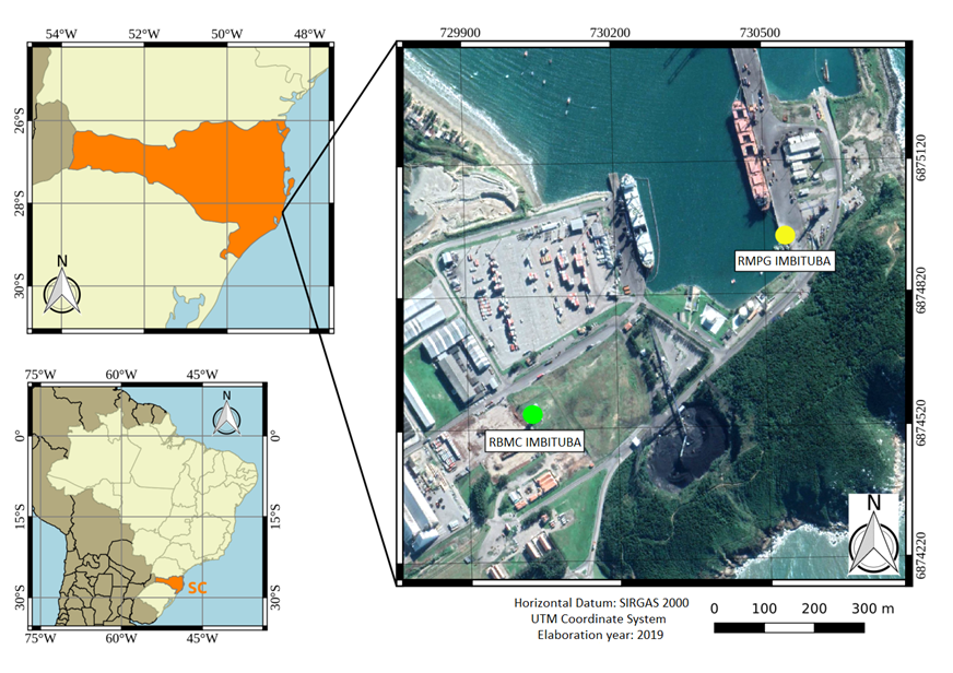
2.1 Study area

Figure 1 shows the location of the tide gauge station and the GNSS continuous monitoring station in Imbituba. The two stations are located approximately 650 meters apart.

Figure 1:
Location of the RMPG Tide Gauge and the RBMC GNSS Station in Imbituba.

We delimited the area of the altimetric observations based on the studies of Garcıa et al. (2011); and Montecino et al. (2017), who analyzed an area that allowed obtaining Sea Surface Height (SSH) values over a 500 km radius over the ocean from the tide gauge location. According to the authors, this radius was determined by convoluting the satellite altimetry data into a two-dimensional Gaussian function centered on the tide gauge location. The function assumes the value of 1/2 (half intensity) at a distance of 50 km from the tide gauge and disappears beyond 500 km (no intensity).

2.2 Satellite altimetry time series

The altimetric product employed in this study was SSH, which consists of the difference between the satellite altitude relative to a reference ellipsoid and the satellite altitude relative to the surface of the oceans (Escudier et al. 2017). The SSH values were obtained from the Open Altimeter Database (OpenADB) maintained and created by the Deutsches Geodätisches Forschungsinstitut (DGFI). The data time series covers the period from 1992 to 2017 (Schwatke et al. 2010). We used the data available along the tracks of the TOPEX/POSEIDON, Jason 1, 2, and 3 satellites at a radius of up to 500 km over the ocean from the Imbituba tide gauge location. We demarcated cells for each satellite track, so that each cell contains at least one altimetric observation for each satellite revisit. The cells were 7 km long and 3 km wide. They were defined based on the sampling rate of the satellite altimetry data - 1 Hz. This sampling rate corresponds to a sea level measurement approximately every 7 km along the track (Schwatke et al. 2010).

For the VLM analysis, we analyzed the 15 SSH cells that provided the best correlations with tide gauge data from 2002 to 2015. We chose this time period because calculating the correlation coefficient requires two time series of the same length. Thus, the tide gauge series from 2002 to 2015 was the one that showed no evidence of a change in the source reference of the readings. It is worth mentioning that prior to the correlation analysis, we eliminated SSH outliers using the (3( rule.

Data from satellite altimetry missions processed by OpenADB/DGFI received geophysical corrections according to what was suggested by Bosch et al. (2014). Therefore, in order to consider that the satellite altimetry missions and the tide gauge are observing the same ocean signal, we removed ocean tide and ocean load corrections from the SSH values using an empirical model called EOT11a (Empirical Ocean Tide Model 11a) provided by the DGFI. In addition, we applied atmospheric corrections to the tide gauge data, which will be detailed in section 2.3.

Finally, we applied the linear regression model to the 15 cells that showed a correlation coefficient greater than 0.69 which equates to a moderate to strong correlation according to Shimakura (2006) in order to determine the linear trends of sea level variation observed by satellite altimetry missions in relation to the Earth’s geocenter (v _sa ).

2.3 Tide gauge time series

The water level data detected by the Imbituba tide gauge were acquired for the period from 2002 to 2015. After data acquisition, we removed water level outliers using the (3( rule. Since there were some data gaps in the time series, we chose to fill in the missing data with synthetic tides produced using the observed water level values. The synthetic tides were generated by the ‘tidem’ function installed in the ‘oce’ library, created by Kelley (2019) and available for R programming language. This function extracts the sine and cosine components of the tidal frequencies contained in the tide gauge observations. Based on the resulting coefficients of the sine and cosine terms, we calculated amplitude and phase, which allowed the generation of synthetic tides.

We then applied atmospheric corrections to the tide gauge data. These corrections were generated from the global Dynamic Atmospheric Correction model, which designs the ocean’s barotropic response to wind and atmospheric pressure forces estimated by the Mog2D-G model, for periods shorter than 20 days, and by inverse barometer approximation for longer periods (Fenoglio-Marc et al. (2012); Cipollini et al. (2017)). In sequence the time series were filterd by a low pass filter available in Pugh (1987).

To calculate Pearson’s correlation coefficient, we resampled the tide gauge data to match the temporal resolution interval of the satellite altimetry data. We used the ‘resample’ function provided in the ‘signal’ package for the R programming language (Ligges, 2015). The ‘signal’ package consists of a set of functions for signal processing, which involves filtering, resampling routines, and filter models visualization. The ‘resample’ function allows us to resample the time interval of continuous variables, such as tide gauge time series, from the sum of the normalized cardinal sine function of the neighborhood points (Smith 2002; Smith and Gossett 1984). Finally, we applied the linear regression model to the tide gauge series to determine the trend of sea level variation observed by the tide gauge relative to the earth’s crust (v _TG ).

In contact with the RMPG, the expansion of the port of Imbituba between 2010 and 2012 did not impact the tide gauge, because it is installed in the oldest part of the pier.

2.4 GNSS time series

The SIRGAS Continuously Operating Network (SIRGAS-CON) is materialized by more than 400 continuously operating GNSS stations distributed in the Americas and the Caribbean, whose objective is to provides weekly positions of stations (referred to a specific reference epoch) and their changes with time (station velocities) (SIRGAS 2021). In Brazil, all RBMC stations are part of the SIRGAS-CON network. The establishment and maintenance of RBMC stations are under the responsibility of IBGE.

The SIRGAS also provides the multi-year (cumulative) solutions (positions + velocities) for practical and scientific applications requiring time dependent positioning (SIRGAS 2021). In the present study, the multi-year solutions presented in Table 1 were used for the Imbituba Tide Gauge Station:

Table 1:
SIRGAS Multi-year solutions.

Multi-year solutions	Satellite systems	Aligned to	Epoch	Time span	Reference
SIR10P01	GPS	ITRF2008	2005.0	2007-09-05 thru 2010-06-05	Seemüller et al. (2010)
SIR11P01	GPS	ITRF2008	2005.0	2007-09-05 thru 2011-04-16	Sánchez and Seitz (2011a) and Sánchez and Seitz (2011b)
SIR15P01	GPS and GLONASS	IGb08	2013.0	2010-03-14 thru 2015-04-11	Sánchez and Drewes (2016a) and Sánchez and Drewes (2016b)
SIR17P01	GPS and GLONASS	IGS14	2015.0	2011-04-17 thru 2017-01-28	Sánchez and Drewes (2020a) and Sánchez and Drewes (2020b)

2.5 Integration of tide gauge and satellite altimetry data

While tide gauge and satellite altimetry observations are subject to the many variations that affect sea level, tide gauges, as they are fixed to the earth’s crust, also record tectonic movements. Considering this context, we aimed to determine the absolute VLM trend (v_U) in the tide gauge region by the difference between v _SA and v _TG , as presented in Equation (1) (Nerem and Mitchum 2002; Montecino et al. 2017):

$v_U=v_{SA}-v_{TG}$ (1)

The values of (v _SA ) and (v _TG ) were determined from the linear regression model. Therefore, the noise for tide gauge and satellite altimetry time series regression is assumed to be white and uncorrelated. According to Moore (2010), linear regression aims to find a mathematical relationship of a set of random data, usually in the form of a straight line. Suppose that h(t) is the dependent variable (plotted on the vertical axis), t and t ₀ are the independent variables (plotted on the horizontal axis) which in the case for time series corresponds to the time difference between instant t and t ₀ . Simple linear regression describes the relationship between h(t) and (t-t ₀ ) through a straight line that has the following form:

$h\left(t\right)=h_0+v(t-t_0)+e$ (2)

where h ₀ is the intercept estimate of a value of h(t) when (t-t ₀ )=0, v is the estimate of the regression slope or vertical velocity and e is the estimate of the residual value.

There are three possible interpretations for the value of v _U , as presented below:

v_U=0: no VLM;

v_U>0: VLM is upward (uplift); and

v_U<0: VLM is downward (subsidence).

The verification of the proposed methodology was performed through the analysis between v _U , determined by equation (1), and v _GNSS .

We determined the values of v _SA , v _TG , and v _GNSS considering two different scenarios, as presented in Table 2. In the first scenario, we considered the maximum time periods for the time series. Here, the satellite altimetry data time series comprises the time period from 1992 to 2017 (OpenADB/DGFI version 33), the tide gauge series comprises the time period from 2002 to 2015 (in this period, there is no indication of change in the source reference of the observations), and the GNSS data series comprises the period from 2007 to 2019 (the Imbituba GNSS station started operating in 2007). In the second scenario, we chose to delimit all time series to September 2007 until December 2015, as this time interval comprises the largest coincident time series of tide gauge, satellite altimetry, and GNSS observations. The overlap between tide gauge and satellite altimetry time series, as presented in Table 2, follows the criteria in Ray et al. (2010), which calls for an overlap of at least five years of data.

Table 2:
Time intervals.

Trend	v SA	v TG
Scenario 1	1992 - 2017	2002 - 2015
Scenario 2	2007 - 2015	2007 - 2015

3. Results

As seen earlier, we correlated the tide gauge data with each SSH cell along the tracks of the TOPEX/Poseidon, JASON 1, 2, and 3. Thus, considering a 500 km radius from the tide gauge, we demarcated 363 cells along tracks 0050, 0076, 0152, 0163, 0228, and 0239.

Figure 2 presents the variation in the value of the correlation coefficient established between the tide gauge data time series and the SSH time series for the period from 2002 to 2015 in each cell. The correlations get higher as the cells get closer to the tide gauge. We observed the highest correlations in the cells located in track 0163.

Figure 2:
Variation of the correlation coefficient along the satellite tracks in relation to tide gauge data from 2002 to 2015.

3.1 Evolution of the sea level trend in Imbituba

The trend of mean sea level variation (v _SA ) presented in Figure 3 derived from the SSH data for each cell within the study area between 1992 and 2017 (Scenario 1). This trend resulted in a sea level rise of around 2 to 3 mm/a, which is close to the global mean sea level trend of 3.3 mm/a ±0.4 mm/a obtained by Nicholls and Cazenave (2010) for the period between 1993 and 2009. For this estimate, we kept the Openadb/DGFI corrections in the SSH data. Figure 3 shows that cells closer to the coast showed larger oscillations in the sea level trend value compared to cells farther from the coast.

Figura 3:
Sea level trend measured by satellite altimetry in the study area from 1992 to 2017.

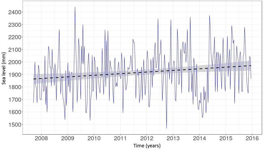
By analyzing the regression line of tide gauge data between 2002 and 2015 (Scenario 1), presented in Figure 4, we found a mean sea-level trend of 5.4 mm/a ±1.9 mm/a. For the period from 2007 to 2015 (Scenario 2), we estimated a sea-level of 13.0 mm/a ± 4.2 mm/a, as shown in Figure 5. Between the middle of 2013 and the middle of 2014 there was an apparent decrease and then a rise in sea level. Therefore, it is important that the period of time covered in the mean sea level analysis is as long as possible. In addition, further studies about possible instrumental effects on the tide gauge data time series are needed.

Figure 4:
Sea level trend measured by tide gauge in Imbituba from 2002 to 2015.

Figure 5:
Sea level trend measured by tide gauge in Imbituba from 2007 to 2015.

For the VLM analysis, we selected the 15 SSH cells that presented the highest correlation with the tide gauge data from Imbituba between 2002 and 2015. Tables 3 and 4 present the results we obtained considering scenarios 2 and 1, respectively.

Table 3 presents the results of v _TG and v _SA between September 2007 and December 2015 (Scenario 2). The mean values of v _TG and v _SA were 13.0 mm/a ± 4.2 mm/a and 7.1 mm/a ± 4.6 mm/a, respectively. The negative signs of v _U characterize a descendent VLM of the crust, i.e., possible crustal subsidence.

Table 3:
Linear regression results of tide gauge and satellite altimetry data between September 2007 and December 2015 and difference between tide gauge and altimetry data.

Center position of the cell	Correlation Coefficient	Dist. km	mm/a 2007 − 2015	mm/a 2007 − 2015	mm/a 2007 − 2015
26°19 ‘32.16” S	0.71	299.9	6.2 ± 5.0	13.0 ± 4.2	-6.8 ± 6.6
46°29 ‘59.04” W
26°26 ‘47.87” S	0.71	286.4	9.1 ± 5.0	13.0 ± 4.2	-3.9 ± 6.5
46°33 ‘26.58” W
26°43 ‘56.52” S	0.70	254.9	7.3 ± 4.7	13.0 ± 4.2	-5.7 ± 6.3
46°41 ‘40.09” W
26°23 ‘12.63” S	0.69	293.0	8.5 ± 4.8	13.0 ± 4.2	-4.5 ± 6.4
46°31 ‘44.28” W
26°33 ‘49.55” S	0.69	273.4	4.6 ± 4.7	13.0 ± 4.2	-8.4 ± 6.3
46°36 ‘48.71” W
26°36 ‘55.76” S	0.69	267.7	6.2 ± 4.7	13.0 ± 4.2	-6.8 ± 6.3
46°38 ‘17.48” W
27°4 ‘56.49” S	0.69	217.5	8.2 ± 4.4	13.0 ± 4.2	-4.7 ± 6.1
46°51 ‘47.90” W
26°47 ‘40.33” S	0.69	248.1	9.5 ± 4.6	13.0 ± 4.2	-3.5 ± 6.2
46°43 ‘26.80” W
26°40’14.45 “ S	0.69	261.6	6.1 ± 4.8	13.0 ± 4.2	-6.9 ± 6.4
46°39 ‘52.73” W
26°30 ‘24.37” S	0.69	279.7	8.2 ± 4.8	13.0 ± 4.2	-4.8 ± 6.4
46°35 ‘10.08” W
27°8 ‘28.27” S	0.69	211.4	6.2 ± 4.3	13.0 ± 4.2	-6.8 ± 6.0
46°53 ‘29.63” W
27°18 ‘36.51” S	0.69	194.2	5.1 ± 4.3	13.0 ± 4.2	-7.9 ± 6.0
46°58 ‘25,95” W
27°22 ‘11.47” S	0.68	188.3	9.0 ± 4.3	13.0 ± 4.2	-4.0 ± 6.1
47°00’10.84 “ W
26°51 '15.74" S	0.68	241.7	5.6 ± 4.6	13.0 ± 4.2	-7.4 ± 6.3
46°45 '10.52" W
28°00 '36.24" S	0.68	133.3	5.9 ± 4.2	13.0 ± 4.2	-7.1 ± 5.9
47°19 '01.13" W
Mean	0.69	243.4	7.1 ± 4.6	13.0 ± 4.2	-5.9 ± 6.3

Table 4 presents the results of v _TG and v _SA for the periods 2002 to 2015; 1992 to 2017, respectively (Scenario 1). The mean values of v _TG and v _SA were 5.4 mm/a ± 1.9 mm/a and 2.5 mm/a ± 1.2 mm/a, respectively.

Table 4:
Linear regression results of tide gauge and satellite altimetry data for different time intervals and difference between tide gauge and altimetry data.

Center position of the cell	Correlation Coefficient	Dist. km	mm/a 1992 − 2017	mm/a 2002 − 2015	mm/a
26°19 ‘32.16” S	0.71	299.9	2.1 ± 1.3	5.4 ± 1.9	-3.3 ± 2.3
46°29 ‘59.04” W
26°26 ‘47.87” S	0.71	286.4	2.9 ± 1.3	5.4 ± 1.9	-2.5 ± 2.3
46°33 ‘26.58” W
26°43 ‘56.52” S	0.70	254.9	2.6 ± 1.0	5.4 ± 1.9	-2.8 ± 2.1
46°41 ‘40.09” W
26°23 ‘12.63” S	0.69	293.0	3.0 ± 1.1	5.4 ± 1.9	-2.4 ± 2.2
46°31 ‘44.28” W
26°33 ‘49.55” S	0.69	273.4	1.8 ± 1.0	5.4 ± 1.9	-3.7 ± 2.2
46°36 ‘48.71” W
26°36 ‘55.76” S	0.69	267.7	1.7 ± 1.3	5.4 ± 1.9	-3.8 ± 2.3
46°38 ‘17.48” W
27°4 ‘56.49” S	0.69	217.5	2.6 ± 0.9	5.4 ± 1.9	-2.8 ± 2.1
46°51 ‘47.90” W
26°47 ‘40.33” S	0.69	248.1	3.9 ± 1.2	5.4 ± 1.9	-1.5 ± 2.2
46°43 ‘26.80” W
26°40’14.45 “ S	0.69	261.6	1.7 ± 1.2	5.4 ± 1.9	-3.7 ± 2.3
46°39 ‘52.73” W
26°30 ‘24.37” S	0.69	279.7	3.0 ± 1.3	5.4 ± 1.9	-2.4 ± 2.3
46°35 ‘10.08” W
27°8 ‘28.27” S	0.69	211.4	2.6 ± 1.2	5.4 ± 1.9	-2.8 ± 2.2
46°53 ‘29.63” W
27°18 ‘36.51” S	0.69	194.2	1.4 ± 0.9	5.4 ± 1.9	-4.0 ± 2.1
46°58 ‘25,95” W
27°22 ‘11.47” S	0.68	188.3	2.0 ± 0.9	5.4 ± 1.9	-3.5 ± 2.1
47°00’10.84 “ W
26°51 ‘15.74” S	0.68	241.7	2.1 ± 1.2	5.4 ± 1.9	-3.3 ± 2.2
46°45 ‘10.52” W
28°00 ‘36.24” S	0.68	133.3	3.6 ± 1.8	5.4 ± 1.9	-1.8 ± 2.6
47°19 ‘01.13” W
Mean	0.69	243.4	2.5 ± 1.2	5.4 ± 1.9	-3.0 ± 2.2

The mean regression standard errors for the values of v _SA were ±4.6 mm/a and ±1.2 mm/a for the time periods of 2007 to 2015 (Table 3) and 1992 to 2017 (Table 4), respectively. This demonstrates that using longer time series of satellite altimetry data allows for more consistent results to quantify sea level variation. We also found lower mean error values in v _TG in longer time series: ±4.2 mm/a and ±1.9 mm/a for the time periods of 2007 to 2015 (Table 3) and 2002 to 2015 (Table 4), respectively.

Table 3 and 4 presents a mean correlation of 0.69 between 2002 and 2015. All 15 cells were located along pass 0163 and at a mean distance of 243.4 km from the tide gauge. We did not extrapolate the satellite altimetry data to the coast nor correct instrumental drift errors contained in the tide gauge observations. These aspects are under study and will be considered in future studies.

The root mean squared error (RMSE) results of the residues were 167.1 mm and 175.3 mm for the between 2002 and 2015 and between 2007 and 2015, respectively. The longest time series (2002-2015) showed a closer approximation between the observed values and those predicted by the linear regression model.

All the values of v _U shown in Tables 4 and 5 are negative, which means that the values of were greater than v _SA . An analysis of mean sea level at RMPG stations between 2001 and 2015, conducted by IBGE, found a systematic effect on tide gauge data due to tide gauge sensor drift or instrumental drift at the Imbituba station (IBGE 2016). This may influence the results we presented, in this way more studies about the instrumental effect should be carried out in the future, as well as studies about the extrapolation of satellite altimetry data to the coast, in order to allow a comparison of time series for the same geographical position.

Table 5 presents the values of v _GNSS related to four SIRGAS Multi-year solutions at different periods: SIR10P01 (2007-2010), SIR11P01 (2007-2011), SIR15P01 (2010-2015), and SIR17P01 (2011-2017). It was noted that v _GNSS showed close values for the time periods with the most overlapping data, that is, SIR10P01 (2007-2010) and SIR11P01 (2007-2011) solutions had values of -0.8 mm/a ± 0.3 mm/a and - 0.1 m/a ± 1.7 mm/a, respectively, while solutions SIR15P01 (2010-2015) and SIR17P01 (2011-2017) had values of -3.4 mm/a ± 0.3 mm/a and -2.0 mm/a ± 0.7 mm/a, respectively. All solutions presented a trend of crustal subsidence in Imbituba.

Table 5:
VLM estimated from SIRGAS Multi-year solutions in Imbituba.

Multi-year solutions	Time span	(mm/a)
SIR10P01	2007-09-05 thru 2010-06-05	-0.8 ± 0.3
SIR11P01	2007-09-05 thru 2011-04-16	- 0.1 ± 1.7
SIR15P01	2010-03-14 thru 2015-04-11	-3.4 ± 0.3
SIR17P01	2011-04-17 thru 2017-01-28	-2.0 ± 0.7

When analyzing Table 3, 4 and 5, it is noted that the values of v _GNSS obtained from the Multi-year solutions SIR15P01 and SIR17P01 (-3.4 mm/a ± 0.3 mm/a and -2.0 mm/a ± 0.7 mm/a, respectively) were close to the values of v _U (mean -3.0 mm/a ± 2.2 mm/a) presented in Table 4 in relation to the values of v _U (mean -5.9 mm/a ± 6.3 mm/a) presented in Table 3. This fact demonstrates that the use of longer series of tide gauge, satellite altimetry and GNSS, tends to produce more consistent results.

4. Conclusion

The mean values of v _U for the period from 2007 to 2015 and for other periods (v _SA (1992-2017) - v _TG (2002-2015)) were -5.9 mm/a ±6.3 mm/a and -3.0 mm/a ±2.2 mm/a. The mean values of v _GNSS were also negative in all periods of time we analyzed. Hence, the negative signs indicate that the VLM in the region of Imbituba is in the downward direction, i.e., they indicate possible crustal subsidence in that region. The comparison of VLM obtained between v _U and v _GNSS showed results with better consistency over longer time series, that is, the v _GNSS values from the Multi-year solutions SIR15P01 and SIR17P01 were close to the values of v _U determined by the difference between v _SA (1992-2017) and v _TG (2002-2015).

Regarding mean sea level variation, we observed that the mean values for v _SA (1992-2017) and v _TG (2002-2015) were 2.5 mm/a ±1.2 mm/a and 5.4 mm/a ± 1.9 mm/a, respectively, while the mean values for v _SA (2007-2015) and v _TG (2007-2015) were 7.1 mm/a ± 4.6 mm/a and 13.0 mm/a ±4.2 mm/a. The use of longer SSH time series and tide gauge data allowed us to reduce the value of the regression standard error, which provides a closer match of the regression line to the observed data.

As for recommendations for future studies, we suggest considering the temporal and spatial variations of the sea surface between the tide gauge station and the SSH cells. In addition, we advise analyzing other tide gauges belonging to the RMPG in order to verify the methodology employed in this study.

ACKNOWLEDGMENT

This study was carried out with the support of the Coordination for the Improvement of Higher Education Personnel (CAPES) - Funding Code 001. The authors would like to thank the Academic Publishing Advisory Center (Centro de Assessoria de Publicação Acadêmica, CAPA - www.capa.ufpr.br) of the Federal University of Paraná (UFPR) for assistance with English language translation and developmental editing.

REFERENCES

• Barnett, T. P. 1984. The estimation of “global” sea level change: a problem of uniqueness. Journal of Geophysical Research: Oceans 89 (C5), pp. 7980-7988.
• Bosch, W. Dettmering, D. and Schwatke, C. 2014. Multi-Mission Cross- Calibration of Satellite Altimeters: Constructing a Long-Term Data Record for Global and Regional Sea Level Change Studies. Remote Sensing 6 (3), pp. 2255- 2281. DOI: 10.3390/rs6032255.
  » https://doi.org/10.3390/rs6032255
• Montecino, H. D., Ferreira, V. G., Cuevas, A., Cabrera, L. C., Báez, J. C. S. and De Freitas, S. R. 2017. Vertical deformation and sea level changes in the coast of Chile by satellite altimetry and tide gauges. International Journal of Remote Sensing 38(24), pp. 7551-7565. DOI: 10.1080/01431161.2017.1288306.
  » https://doi.org/10.1080/01431161.2017.1288306
• Cipollini, P., Calafat, F. M., Jevrejeva, S., Melet, A. and Prandi, P. 2017. Monitoring Sea Level in the Coastal Zone with Satellite Altimetry and Tide Gauges. Surveys in Geophysics 38 (1), pp. 33-57. DOI: 10. 1007/s10712-016-9392-0.
  » https://doi.org/10. 1007/s10712-016-9392-0
• Da Silva, L. M., & de Freitas, S. R. C. (2019). Análise da evolução temporal do Datum Vertical Brasileiro de Imbituba [Analysis of the temporal evolution of the Imbituba Brazilian Vertical Datum].Revista Cartográfica, (98), pp. 33-57. DOI: 10.35424/rcarto.i98.140.
  » https://doi.org/10.35424/rcarto.i98.140
• Da Silva, L. M. and De Freitas, S. R. C. 2014. Análise da variação temporal do nível médio do mar nas estações da RMPG [Analysis of the temporal variation of the mean sea level in the RMPG stations]. In: Symposium SIRGAS 2014 (La Paz, Bolivia).
• Dalazoana, R. 2006. Estudos dirigidos à análise temporal do Datum Vertical Brasileiro [Studies aimed at the temporal analysis of the Imbituba Brazilian Vertical Datum].Boletim de Ciências Geodésicas, 12 (1), pp.173-174.
• Escudier, P., Couhert, A., Mercier, F., Mallet, A., Thibaut, P., Tran, N., Amarouche, L., Picard, B., Carrere, L., Dibarboure, G., Ablain, M., Richard, J., Steunou, N., Dubois, P., Rio, M. H. and Dorandeu, J. 2017. Satellite Radar Altimetry: Principle, Accuracy, and Precision. In: Satellite altimetry over oceans and land surfaces CRC Press, pp. 1-70.
• Fenoglio-Marc, L., Braitenberg, C. and Tunini, L. 2012. Sea level variability and trends in the Adriatic Sea in 1993-2008 from tide gauges and satellite altimetry. Physics and Chemistry of the Earth 40 - 41, pp. 47-58. DOI: 10.1016/j.pce. 2011.05.014
  » https://doi.org/10.1016/j.pce. 2011.05.014
• Garcıa, F. Vigo, M. I. Garcıa-Garcıa, D. and Sánchez-Reales, J. M. 2011. Combination of Multisatellite Altimetry and Tide Gauge Data for Determining VLMs along Northern Mediterranean Coast. Pure and Applied Geophysics 169 (8), pp. 1411-1423, DOI:10.1007/s00024-011-0400-5.
  » https://doi.org/10.1007/s00024-011-0400-5
• IBGE, Instituto Brasileiro de Geografia e Estatística 2016. Análise do Nível Médio do Mar nas Estações da Rede Maregráfica Permanente para Geodésia - RMPG 2001/2015 [Analysis of the Mean Sea Level at Rede Maregráfica Permanente para Geodésia - RMPG 2001/2015] Rio de Janeiro. Available at: <Available at: http://geoftp.ibge.gov.br/informacoes_sobre_posicionamento_geodesico/rmpg/relatorio/relatorio_RMPG_2001_2015_GRRV.pdf > [Accessed 02 May 2020].
  » http://geoftp.ibge.gov.br/informacoes_sobre_posicionamento_geodesico/rmpg/relatorio/relatorio_RMPG_2001_2015_GRRV.pdf
• Kelley, D. E. 2019. Analysis of Oceanographic Data Available at: <Available at: https://www.rdocumentation.org/packages/oce/versions/1.1-1 > [Accessed 20 October 2019].
  » https://www.rdocumentation.org/packages/oce/versions/1.1-1
• Ligges, U. 2015. Signal Processing Available at: <Available at: https://www.rdocumentation.org/packages/signal > [Accessed 05 May 2020].
  » https://www.rdocumentation.org/packages/signal
• Moore, D. S. 2010. Basic Practice of Statistics, 5th Edition New York: W. H. Freeman e Company.
• Nerem, R. S. and Mitchum, G. T. 2002. Estimates of Vertical Crustal Motion Derived from Differences of TOPEX/POSEIDON and Tide Gauge Sea Level Measurements. Geophysical Research Letters 29 (19), pp. 40-1-40-4. DOI: 10.1029/2002gl015037.
  » https://doi.org/10.1029/2002gl015037
• Nicholls, R. J. and Cazenave, A. 2010. Sea-Level Rise and Its Impact on Coastal Zones. Science 328 (5985), pp. 1517-1520. DOI: 10.1126/science.1185782.
  » https://doi.org/10.1126/science.1185782
• PBMC, Painel Brasileiro de Mudanças Climáticas 2016. Impacto, vulnerabilidade e adaptação das cidades costeiras brasileiras às mudanças climáticas: Relatório Especial do Painel Brasileiro de Mudanças Climáticas [Impact, vulnerability and adaptation of Brazilian coastal cities to climate change: Special Report of the Brazilian Panel on Climate Change] UFRJ. Rio de Janeiro, Tech. rep., p. 184. Available at: <Available at: https://www.researchgate.net/publication/328388678_Impacto_vulnerabilidade_e_adaptacao_das_cidades_costeiras_brasileiras_as_mudancas_climaticas_Relatorio_Especial_do_Painel_Brasileiro_de_Mudancas_Climaticas > [Accessed 06 May 2020].
  » https://www.researchgate.net/publication/328388678_Impacto_vulnerabilidade_e_adaptacao_das_cidades_costeiras_brasileiras_as_mudancas_climaticas_Relatorio_Especial_do_Painel_Brasileiro_de_Mudancas_Climaticas
• Plag, H. P., Altamimi, Z., Bettadpur, S., Beutler, G., Beyerle, G., Cazenave, A., Crossley, D., Donnellan, A., Forsberg, R., Gross, R., Hinderer, J., Komjathy, A., Ma, C., Mannucci, A. J., Noll, C., Nothnagel, A., Pavlis, E. C., Pearlman, M., Poli, P., Schreiber, U., Senior, K., Woodworth, P. L., Zerbini, S. and Zuffada, C. 2009. The goals, achievements, and tools of modern geodesy. In: Global Geodetic Observing System: Meeting the Requirements of a Global Society on a Changing Planet in 2020 Berlin, Heidelberg: Springer Berlin Heidelberg, pp. 15-88. DOI: 10.1007/978-3-642-02687-4_2.
  » https://doi.org/10.1007/978-3-642-02687-4_2
• Prates, A. P. L., Gonçalves, M. A. and Rosa, M. R. 2012. Panorama da Conservação dos Ecossistemas Costeiros e Marinhos no Brasil [Overview of the Conservation of Coastal and Marine Ecosystems in Brazil] Brasília: Ministério do Meio Ambiente, Secretaria de Biodiversidade e Florestas, Gerência de Biodiversidade Aquática e Recursos Pesqueiros, p. 152. Available at: <Available at: https://www.terrabrasilis.org.br/ecotecadigital/images/abook/pdf/2016/15-Panorama%20da%20Conservao.pdf > [Accessed 12 May 2020].
  » https://www.terrabrasilis.org.br/ecotecadigital/images/abook/pdf/2016/15-Panorama%20da%20Conservao.pdf
• Pugh, D. T. 1987. Tides, Surges and Mean Sea-Level Swindon: John Wiley Sons, p. 472.
• Ray, R. D., B. Beckley, D. and Lemoine, F. G. 2010. Vertical crustal motion derived from satellite altimetry and tide gauges, and comparisons with DORIS measurements. Advances in Space Research 45 (12), pp. 1510-1522. DOI: 10. 1016/j.asr.2010.02.020.
  » https://doi.org/10. 1016/j.asr.2010.02.020
• Sánchez L. and Drewes H. 2016a. SIR15P01: Multiyear solution for the SIRGAS Reference Frame, open access. DOI: 10.1594/PANGAEA.862536.
  » https://doi.org/10.1594/PANGAEA.862536
• Sánchez L. and Drewes H. 2016b. Crustal deformation and surface kinematics after the 2010 earthquakes in Latin America. Journal of Geodynamics 102, pp. 1-23. DOI: 10.1016/j.jog. 2016.06.005.
  » https://doi.org/10.1016/j.jog. 2016.06.005
• Sánchez L. and Drewes H. 2020a.SIRGAS 2017 reference frame realization SIR17P01, open access. DOI: 10.1594/PANGAEA.912349.
  » https://doi.org/10.1594/PANGAEA.912349
• Sánchez L. and Drewes H. 2020b. Geodetic monitoring of the variable surface deformation in Latin America. International Association of Geodesy Symposia Series, 152. DOI: 10.1007/1345_2020_91.
  » https://doi.org/10.1007/1345_2020_91
• Sánchez, L. and Seitz, M. 2011a. SIRGAS reference frame realization SIR11P01 Deutsches Geodätisches Forschungsinstitut der Technischen Universität München, PANGAEA, DOI: 10.1594/PANGAEA.835100.
  » https://doi.org/10.1594/PANGAEA.835100
• Sánchez, L. and Seitz, M. 2011b. Recent activities of the IGS Regional Network Associate Analysis Centre for SIRGAS (IGS RNAAC SIR) - Report for the SIRGAS 2011 General Meeting August 8 - 10, 2011. Heredia, Costa Rica. DGFI Report, 87, 48 pp. Available at: <Available at: https://www.sirgas.org/fileadmin/docs/DGFI_Report_87.pdf > [Accessed 15 December 2021].
  » https://www.sirgas.org/fileadmin/docs/DGFI_Report_87.pdf
• Schwatke, C. Bosch, W. Savcenko, R. and Dettmering, D. 2010. OpenADB - An open database for multi-mission altimetry EGU, Vienna, Austria EGU 2010. Poster. Vienna, Austria.
• Seemüller W., Sánchez L., Seitz M. and Drewes H. (2010).The position and velocity solution SIR10P01 of the IGS Regional Network Associate Analysis Centre for SIRGAS (IGS RNAAC SIR) DGFI Report No. 86, Munich. Available at: <Available at: http://www.sirgas.org/fileadmin/docs/SIR10P01_DGFI_Report_86.pdf > [Accessed 15 December 2021].
  » http://www.sirgas.org/fileadmin/docs/SIR10P01_DGFI_Report_86.pdf
• Shimakura, S. (2006) Interpretação do coeficiente de correlação [Interpretation of the correlation coefficient] Departamento de Estatıstica UFPR. CE003-Estatıstica II. Available at: <Available at: http://leg.ufpr.br/~silvia/CE003/node74.html > [Accessed on: 5 May 2022].
  » http://leg.ufpr.br/~silvia/CE003/node74.html
• Smith, J. 2002. Digital audio resampling home page Available at: <Available at: ccrma.stanford.edu/~jos/resample/ > [Accessed 10 May 2020].
  » ccrma.stanford.edu/~jos/resample/
• Smith, J. and P. Gossett (1984). A flexible sampling-rate conversion methodIn: ICASSP ’84. IEEE International Conference on Acoustics, Speech, and Signal Processing Vol. 9, pp. 112-115. DOI: 10.1109/ICASSP.1984.1172555.
  » https://doi.org/10.1109/ICASSP.1984.1172555

• Erratum

  On the first page, where it reads:
  Samoel Gehl
  Should read:
  Samoel Giehl
  On the first page, in “How to cite this article”, where it reads:
  GEHL, S.
  Should read:
  GIEHL, S.
  On the top of the pages 3, 5, 7, 9, 11, 13, where it reads:
  Gehl and Dalazoana
  Should read:
  Giehl and Dalazoana
  Bulletin of Geodetic Sciences, 28(3): e2022011, 2022

• Erratum

  Page 11, where it reads:
  When analyzing Table 3, 4 and 5, it is noted that the values of obtained from the Multi-year solutions SIR15P01 and SIR17P01 (-3.4 mm/a ± 0.3 mm/a and -2.0 mm/a ± 0.7 mm/a, respectively) were close to the values of (mean -3.0 mm/a ± 2.2 mm/a) presented in Table 4 in relation to the values of (mean -5.9 mm/a ± 6.3 mm/a) presented in Table 3. (...)
  Should read:
  When analyzing Table 3, 4 and 5, it is noted that the values of v_GNSS obtained from the Multi-year solutions SIR15P01 and SIR17P01 (-3.4 mm/a ± 0.3 mm/a and -2.0 mm/a ± 0.7 mm/a, respectively) were close to the values of v_U (mean -3.0 mm/a ± 2.2 mm/a) presented in Table 4 in relation to the values of v_U (mean -5.9 mm/a ± 6.3 mm/a) presented in Table 3. (...)
  Bulletin of Geodetic Sciences, 28(4): e2022020, 2022.

Publication Dates

• Publication in this collection
  01 July 2022
• Date of issue
  2022

History

• Received
  17 Aug 2021
• Accepted
  18 May 2022