Modeling and forecasting international tourism demand in Puno-Peru

Modelagem e previsão da procura por turismo internacional em Puno-Peru

Abstract

The tourism industry in Peru generates about 1.1 million jobs and contributes 3.3% of GDP, which makes it one of its main economic activities, so tourism is no longer just a commercial activity and transforms into a tool for the development of the Peruvian population especially in regions with high poverty rate and with numerous tourist attractions as it is the case of the Puno region with a poverty rate of 24.2% that is located in the south of the country and that has numerous tourist attractions of natural, historical, cultural, and gastronomic type. The objective of this research is to model and forecast the demand of international tourists visiting Puno using the ARIMA methodology of Box-Jenkins, for this the study considers monthly arrival information of foreign tourists between the years 2003 to 2017. Finally, using the statistics MAPE, Z, r, Akaike Information Criterion (AIC) and Schwarz Criterion (SC) was identified to the SARIMA (6, 1, 24)(1, 0, 1)12 model as the most efficient for modeling and forecasting the demand for international tourism in the Puno region.

Keywords:
Seasonality; Titicaca lake; Peru; ARIMA; Culture

Resumo

A indústria do turismo no Peru gera aproximadamente 1.1 milhão de empregos e contribui com 3.3% do PIB, o que a torna uma de suas principais atividades econômicas, portanto o turismo não é mais apenas uma atividade comercial mas é uma ferramenta para o desenvolvimento da população peruana, especialmente nas regiões com alto índice de pobreza e muitas atrações turísticas como é o caso da região de Puno com uma taxa de pobreza de 24.2% localizada no sul do país e com muitas atrações históricas, naturais, cultural e gastronômico. O objetivo desta pesquisa é modelar a procura de turistas internacionais que visitam Puno utilizando a metodologia ARIMA de Box-Jenkins, para este estudo considera informações mensais de chegadas de turistas internacionais entre os anos 2003 e 2017. Finalmente, usando estatísticas MAPE, Z, R, Critério de Informação de Akaike (AIC) e Critério de Schwarz (SC) se encontrou ao modelo SARIMA (6, 1, 24)(1, 0, 1)12 como o mais eficiente para a modelação e previsão da procura do Turismo Internacional na região de Puno.

Palavras-chave:
Sazonalidade; lago Titicaca; Peru; ARIMA; Cultura

Resumen

La industria del turismo en el Perú genera cerca de 1.1 millones de puestos de trabajo y aporta el 3.3% del PBI, lo que la convierte en una de sus principales actividades económicas, de esta forma el turismo deja de ser sólo una actividad comercial y se transforma en una herramienta para el desarrollo de la población peruana especialmente en las regiones con alta tasa de pobreza y con numerosos atractivos turísticos como es el caso de la región de Puno con una tasa de pobreza de 24.2% que está ubicada en el sur del país y que cuenta con numerosos atractivos turísticos de tipo naturales, históricos, culturales y gastronómicos. El objetivo de esta investigación es modelar y proyectar la demanda de turistas internacionales que visitan Puno utilizando la metodología ARIMA de Box-Jenkins, para ello el estudio considera información mensual de arribo de turistas internacionales entre los años 2003 a 2017. Finalmente, utilizando los estadísticos MAPE, Z, r, Criterio de Información de Akaike (AIC) y Criterio de Schwarz (SC) se identificó al modelo SARIMA (6, 1, 24)(1, 0, 1)12 como el más eficiente para el modelamiento y proyección de la demanda del turismo internacional en la región de Puno.

Palavras clave:
Estacionalidad; lago Titicaca; Perú; ARIMA; Cultura

1 INTRODUCTION

Considering the natural resources, culture, gastronomy, folklore, history, among others, the tourism industry is increasingly important in the economy of the countries since it is closely related to social and economic development. According to the World Tourism Organization (UNWTO), tourism has grown more rapidly in recent years becoming the third category of export behind chemicals and fuels and ahead of automotive products and food. International tourist arrivals in the world went from 674 million in 2000 to 1,235 million in 2016 and the income recorded by destinations around the world went from 495,000 million dollars in 2000 to 1.22 billion dollars in 2016 (OMT, 2017).

In Peru, this industry generates about 1.1 million jobs and contributes 3.3% of GDP (CAMARA, 2018) where in 2017 the GDP amounted to a value of 157,744 million dollars where the tourism sector represents 3.2% of this total being above the sectors of fisheries, aquaculture, electricity, and natural gas; and showing a growth of 1.4% compared to 2016 (BCRP, 2018), which makes the tourism sector one of its main economic activities due to the fact that same year, 4 million 32 thousand 339 international tourists arrived in the country, representing an 8% growth in incoming tourism compared to 2016 (MINCETUR, 2017a), where the main countries that visited Peru in 2017 were: Chile ( 27%), the United States (15%), Venezuela (5%), Ecuador (7%), Colombia (5%), and Argentina (5%) making a market share of 69% of arrivals to the country (GESTION, 2017). The main entry points to the country were: Jorge Chavez International Airport (58%), Tacna (23%), Tumbes (9%), and Puno (5%) (MINCETUR, 2017b). It is estimated that foreign currency revenues generated by incoming tourism in Peru, during the year 2017, reached 4,574 million dollars, representing a growth of 6% in relation to 2016 (MINCETUR, 2017b).

In recent years, the country has opted for sustainable tourism that promotes policies, practices, and ethical behavior through the efficient use of resources; also, it has sought to promote peace, development, and the eradication of poverty. In this way, tourism ceases to be just a commercial activity and becomes a tool for the development of the Peruvian population, especially in the regions with the highest poverty rate and with numerous tourist attractions such as the Puno region which is the fourth most visited by international tourists (see Figure 1), which to date has a poverty rate of 24.2%, placing it in the tenth poorest region of Peru (INEI, 2018a) and yet is endowed with many tourist attractions that could in the future be exploited more efficiently with sustainable tourism policies.

In 2017, GDP in the Puno region was more than 2,892 million dollars, representing a variation of 3.9% with respect to 2016, where the tourism sector represents 2% of the regional GDP that registered international visits for more than 62.5 million dollars in the same year that is above the fishing, electricity, and gas sector with a growth in 2017 of 2.43% compared to 2016. Likewise, the annual growth of the tourism sector in Puno since 2010 is always positive as well as the agricultural sector that is the most representative sector of GDP in Puno (INEI, 2018b).

Currently, tourism in Puno is important because it benefits hundreds of people, so the tourism sector in the Puno region in 2017 generated more than 90 thousand jobs; and the National Chamber of Tourism (CANATUR) estimates that tourism in 2035 will be one of the first sectors that will generate development and increase employment in the Puno region (CORREO, 2017); hence the importance for companies in the sector to have a good forecasting on the number of arrivals of international tourists in order to carry out a better planning, forecasting, and management of the activity.

Figure 1
Arrival of international visitors to accommodation establishments according to regions of Peru, 2003-2016

As a brief description, the region of Puno is located in southern Peru on the shores of Lake Titicaca-called the "highest navigable lake in the world" (INRENA, 1995) at a height of 3,827 masl with a cold dry climate and it is considered a good tourist destination due to the infrastructure, basic services, location, presence of diverse natural settings (Cayo & Apaza, 2017) and by the creation of new types of tourism in the region as is the case of ecotourism, rural tourism, adventure tourism, experiential tourism, and other forms of so-called alternative tourism mainly in the communities of Amantaní, Pucará, Llachón, Anapía, Atuncolla, and Sillustani where visitors can spend a few days in these communities learning more about their customs and traditions (Mamani, 2016). As main tourist attractions, it has: Lake Titicaca, eco-tourist boardwalk Bahía de los Incas, floating island of Uros (Figure 2), Amantaní Island, Taquile Island, Llachón, among others (PUNO, 2017). On the other hand, the region of Puno offers a diversity of historical-cultural tourist destinations including archaeological remains in various cities, and has a vast diversity in folkloric-cultural resources. Likewise, the region has a wide variety of gastronomic resources in each community.

The main objective of this research is to model and forecast the number of international tourists arriving in Puno through an analysis of the historical series of international tourist arrivals and their seasonal variations using monthly periodicity from 2003 to 2017. This research uses the ARIMA (Auto-Regressive Integrated Moving Average) methodology of Box & Jenkins (1976) for the modeling and forecasting of the statistical series whose usefulness of work is mainly foresight in the operational decisions of tourism, tour preparations, infrastructure, transportation, training in the service, among others. Finally, the document is structured as follows: the theoretical framework is presented, a description of the materials and methods used is made, later the results are presented using the Box-Jenkins methodology and finally the most outstanding conclusions for the present study.

Figure 2
Floating Island of the Uros on Lake Titicaca (3,827 masl) - Puno, Peru

2 LITERATURE REVIEW

In this regard, for the study and forecasting of tourism demand with time series, there are several research works, so for ARIMA modeling there are the works of Hosking (1981), Chang et al., (2009), Loganathan & Ibrahim (2010), Lim & Mcaleer (1999), Peiris (2016), Reisen (1994), Nanthakumar, Subramaniam, & Kogid (2012), Greenidge (2001). For the costs of tourism in ARIMA models, the work of Psillakis, Alkiviadis, & Kanellopoulos (2009); using the ARIMA-GARCH methodology there are the investigations of Coshall (2009), Shareef & McAleer (2005); with models ARMA-GARCH multivariate the work of Chan, Lim, & McAleer (2005). Likewise, works that use the ARFIMA models (ARIMA Fractionally Integrated models) of long memory are the works of Granger & Joyeux (1980), Peiris & Perera (1988), Baillie (1996); ARIMA and ARFIMA models that use the statistician MAPE, MAE and RMSE, are the works of Chu (2008), Shitan (2008) and Lee, Song, & Mjelde (2008); with ARFIMA-FIGARCH models for tourism the works of Chokethaworn et al., (2010) and Ray (1993); with modeling X-12-ARIMA and ARFIMA the work of Chaitip & Chaiboonsri (2015). Regarding the modeling of tourism supply and demand with VECM models, the work of Zhou, Bonham, & Gangnes (2007); or the forecasting of tourism demand in multivariate and univariate series the work of du Preez & Witt (2003). For the modeling and econometric forecasting of the tourism demand by OLS the works of Athanasopoulos & Hyndman (2006) and Botti, Peypoch, Randriamboarison, & Solonandrasana (2007) and for the forecasting of income due to tourism with the ARMAX methodology, the work of Akal (2004).

3 MATERIALS AND METHODS

The selection of materials and methods for the present investigation comprises three parts: the description of the data to be used, the ARIMA methodology, stationarity tests, and tests to choose more efficient models.

3.1. Data

For the development of this research information was used with monthly period for the years 2003 to 2017 extracted from the database of the Central Reserve Bank of Peru - Branch Puno (BCRP) for the total number of international tourist arrivals to the department of Puno.

3.2 Seasonal ARIMA methodology of Box-Jenkins

The seasonal ARIMA model of Box & Jenkins (1976) is used, consisting of the following methodology steps:

Preliminary analysis: perform a preliminary analysis of all the information in such a way that it is a stationary stochastic process.

Identification of a tentative model: in this step, the order (p, d, q) of the ARIMA model is specified, for which correlograms and simple and partial autocorrelation functions are used.

Estimation of the model: the next step is the estimation of the ARIMA model identified in the previous step. The estimate can be made by the method of least squares or maximum likelihood.

Diagnosis of results and selection: for this step, the models are reviewed using statistical tests for parameters and residues. Likewise, the Akaike Information Criterion (AIC) and the Schwarz Information Criterion (SC) are used to choose the best model. On the other hand, it is possible to use the statistic Mean Absolute Percentage Error (MAPE), the percentage of measurement of the result (Z) and the normalized correlation coefficient (r) for the selection of the most efficient model.

Forecasting: if the most efficient model from the previous step is the right one, then the model can be used for representation and projection.

For the definition of the ARIMA model we have the following processes $AR(p)$ and $MA(q)$:

$Y_t={\displaystyle \sum _{i=1}^p{\varphi }_i{Y}_{t-i}+{\epsilon }_t},$

$Y_t={\epsilon }_t+{\displaystyle \sum _{i=1}^q{\theta }_i{\epsilon }_{t-i}}.$

A model$ARIMA(\mathrm{0,}d\mathrm{,0})$ is a time series that becomes a white noise process after being differentiated $d$ times. The model $ARIMA(\mathrm{0,}d\mathrm{,0})$ is expressed as ${(1-L)}^d{Y}_t={\epsilon }_t$ or what is the same as $Y_t-Y_{t-d}={\epsilon }_t$. The general formulation of a model $ARIMA(p,d,q)$ is called the integrated process of moving averages of order $(p,d,q)$ and is written as

$Y_t-Y_{t-d}={\displaystyle \sum _{i=1}^p{\varphi }_i{Y}_{t-i}+{\epsilon }_t}+{\displaystyle \sum _{i=1}^q{\theta }_i{\epsilon }_{t-i}}$

or in its compact form,

$(1-{\varphi }_{1}L-{\varphi }_2{L}^2-\cdots -{\varphi }_p{L}^p){(1-L)}^d{Y}_t=(1-{\theta }_{1}L-{\theta }_2{L}^2-\cdots -{\theta }_q{L}^q){\epsilon }_t$

The series with secular tendency and cyclical variations can be represented with the $ARIMA(p,d,q)(P,D,Q)$ or $SARIMA(p,d,q)(P,D,Q)$ models. The first parenthesis refers to the secular trend or regular part and the second parenthesis to the seasonal variations or cyclic part of the series.

3.3 Stationarity tests

3.3.1 Unit root test of Augmented Dickey-Fuller (ADF)

The ADF test of Dickey & Fuller (1979) seeks to determine the existence of a unit root in a series of time. The null hypothesis of this test is that there is a unit root in the series. In a simple autoregressive model of order one, AR (1):

$y_t=\rho y_{t-1}+u_t$

where $y_t$ is the variable of interest, $t$ is the time variable, $\rho$is a coefficient, and $u_t$ is the error term. The unit root is present if $\rho =1$. In this case, the model would not be stationary. The regression model can be written as:

$\Delta y_t=(\rho -1)y_{t-1}+u_t=\delta y_{t-1}+u_t$

where $\Delta$ is the operator of the first difference. This model can be estimated and the tests for a unit root are equivalent to $\delta =0$ tests (where $\delta =\rho =-1$). Since the test is performed with the residual data instead of the raw data, it is not possible to use a standard distribution to provide critical values. Therefore, this statistic has a certain distribution known simply as the table of Dickey & Fuller (1979).

3.3.2 Phillips-Perron unit root test (PP)

The PP test of Phillips & Perron (1988) is a unit root test and is used in the analysis of time series to test the null hypothesis that a time series is integrated in order 1. It is based on the Dickey & Fuller (1979) with the null hypothesis is $\rho =0$ in $y_t=\rho y_{t-1}+u_t$ where $\Delta$is the first difference of the operator. Like the augmented Dickey-Fuller test, the Phillips-Perron test addresses the issue that the data generation process for $y_t$could have a higher order of autocorrelation that is admitted into the test equation by making endogenous ARIMA and invalidating so the Dickey-Fuller t-test. While the augmented Dickey-Fuller test addresses this issue by introducing $\Delta y_t$ delays as independent variables in the test equation, the Phillips-Perron test makes a nonparametric correction to the t-test statistic.

3.4 Selection tests of the optimal models

3.4.1 Akaike Information Criterion (AIC)

The Akaike Information Criterion was developed by Akaike (1974) and is a measure for the selection of the best estimated model. In the general case, you can write the equation as

$AIC=2k-2\ln (L)$

where k is the number of parameters in the statistical model and L is the value of the maximum likelihood function for the estimated model.

3.4.2 Schwarz Information Criterion (SC)

The Bayes Information Criterion (BIC) or Schwarz Information Criterion (SC) was developed by Schwarz (1978) and is a criterion for choosing the best model among a class of parametric models with different number of parameters. In the general case, it is written as

$-2\ln p(x|k)\approx BIC=-2\ln l$

where n is the number of observations or the sample size, k is the number of free parameters to be estimated including the constant and L the maximized value of the likelihood function.

3.4.3 Mean Absolute Percentage Error (MAPE)

The Mean Absolute Percentage Error (MAPE) is a measure of the occurrence of a time series. This is always expressed as a percentage, the formula of the MAPE statistic is as follows:

$MAPE=\frac{1}{n}{\displaystyle \sum _{i=1}^n\left|\frac{A_i-F_i}{A_i}\right|}$

where $A_i$ is the current value and $F_i$ is the forecasting value. The difference between $A_i$ and $F_i$ is divided by the current value of $A_i$. The absolute value of this calculation is added for each observation projected in time and divided by the number of observations n. This makes it a percentage error, so you can compare the error of adjusted time series that differ in level. The interpretation for the MAPE guidelines is as follows: if the MAPE value is less than 10% it is a "highly accurate" forecast. If the MAPE value is between 10% and 20% it is a "good" forecast. If the value of MAPE is between 20 and 50% it is a "reasonable" forecast. If the value of MAPE is higher than 50% it is an "inaccurate" forecast (Lewis, 1982).

3.4.4 Percentage of measurement of the result (Z)

The value of Z is used as a relative measure for acceptance levels. As a reference point for the optimal experimental results, Z will be used at a value of $\pm 5\%$, in this way the statistic is defined as:

$Z=\frac{{\displaystyle \sum _{i=1}^{n}j}}{n}*100\%for\{\begin{array}{l}j=1if\left|\frac{A_i-F_i}{A_i}\right|<0.01\\ j=0ifotherwise\end{array}$

where $A_i$ is the current value and $F_i$ is the forecasting value and n the number of observations used. For the choice of the best model should be considered one that has a greater Z value.

3.4.5 Standard correlation coefficient (r)

The normalized correlation coefficient r is a measure of the closeness of the observations and their forecasting is defined as:

$r=\frac{{\displaystyle \sum _{i=1}^n{A}_i*F_i}}{\sqrt{{\displaystyle {\sum }_{i=1}^n{(A_i)}^2*{\displaystyle {\sum }_{i=1}^n{(F_i)}^2}}}}$

where $A_i$ is the current value and $F_i$ is the forecasting value. To choose the best model, choose the one with the largest r statistic.

4 RESULTS

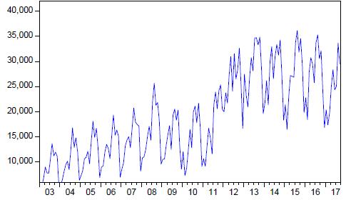
For the presentation of the results, the ARIMA methodology of Box & Jenkins (1976) is used, which consists of the identification, estimation of the model, diagnostic examination and finally the forecasting of the series. The statistical software Eviews 9 was used to analyze the data, using a total of 177 international tourist arrivals with a minimum of 4,650 arrivals and a maximum of 36,147 described in Table 1.

Table 1
Descriptive statistics

Variable	Abbreviation	Obs.	Mean	Stand. Dev.	Min.	Max.
Arrival of international tourists to Puno	arrivals	177	18,809	8,341	4,650	36,147

• Source: The authors

For the identification, Figure 3 shows the evolution of international arrivals in the department of Puno for the years 2003 to 2017, clearly showing a growth and gives evidence to the presence of non-stationarity in mean and variance.

Figure 3
Monthly arrivals of international tourists to Puno, 2003-2017

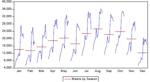
Figure 4 shows that each year arrivals of tourists to Puno have an annual seasonal cycle because they begin to rise from the month of February to May, falling slightly in the month of June recovering in July and reaching its peak in August falling in September recovering slightly in October and falling to a minimum in the month of December. This gives evidence for a 12-month ARIMA seasonal model.

Figure 4
Arrival of international tourists to Puno by stations

4.1. Stationarity tests

As a first step, it is determined if the series is stationary, for this purpose it uses the unit root ADF tests of Dickey & Fuller (1979), PP by Phillips & Perron (1988) and KPSS by Kwiatkowski, Phillips, Schmidt, & Shin (1992) those shown in Table 2.

Table 2
Stationarity tests

Variable	None		With intercept		With intercept and trend
	Level	First difference	Level	First difference	Level	First difference
ADF test	0.716	-2.68**	-1.335	-2.7901	-1.577	-2.868
	(0.868)	(0.007)	(0.612)	(0.061)	(0.798)	(0.175)
PP test	-0.158	-19.742**	-3.345*	-20.061**	-6.313**	-20.003**
	(0.627)	(0.000)	(0.014)	(0.000)	(0.000)	(0.000)
KPSS test	--	--	1.536	0.045**	0.112*	0.041*
	--	--	(0.463)~	(0.463)~	(0.146)~	(0.146)~

• Notes: (*) and (**) denotes statistical significance at 5% and 1%, respectively. Values ​​in () indicate the p-value of Mackinnon (1996). The symbol (~) indicates the critical asymptotic value of Kwiatkowski et al., (1992)
• Source: The authors

Table 2 shows the realization of three different stationarity tests at a level of 1% and 5% level of significance and it is concluded that the arrival of international tourists is not stationary at levels at 1% of significance. For this purpose, the series was calculated in the first difference and as a result, for the PP and KPSS tests, the series is stationary at 1% significance, which indicates that the series is stationary in first difference.

4.2 Autoregressive models and moving averages

The data in logarithms of the arrivals of international tourists to Puno are used to model tourism.

Table 3
Estimation of ARIMA models for the arrival of international tourists to Puno

Variable	Coefficient	t-Statistic	AIC/SC	DW
Model 1
constant	0.006854	2.786144	AIC = -1.179497 SC = -1.017370	2.038498
AR(1)	0.453359	3.636704
AR(3)	0.200060	2.056048
AR(6)	-0.163896	-2.390864
SAR(12)	0.980194	112.742800
MA(1)	-0.890632	-5.971538
MA(24)	-0.109057	-2.232342
SMA(12)	-0.570211	-8.484719
Model 2
constant	0.006666	2.065615	AIC = -1.013858 SC = -0.869745	2.063247
AR(24)	0.697326	12.588560
MA(1)	-0.413207	-4.621061
MA(2)	-0.219508	-2.262754
MA(6)	-0.198948	-2.342499
MA(25)	-0.168337	-1.983791
SMA(12)	0.666660	12.170440
Model 3
constant	0.007537	5.374423	AIC = -0.771678 SC = -0.591537	2.115759
AR(7)	-0.189815	-2.018016
MA(1)	-0.334045	-3.253787
MA(2)	-0.227877	-2.501011
MA(8)	-0.337994	-4.243167
MA(17)	-0.206669	-2.754134
MA(20)	-0.183917	-2.358140
MA(24)	0.325526	2.730460
SMA(12)	0.541756	7.663072
Model 4
constant	0.007277	2.207372	AIC = -0.746528 SC = -0.584401	2.144582
MA(1)	-0.296469	-3.837132
MA(2)	-0.220115	-2.778588
MA(8)	-0.319336	-5.463851
MA(17)	-0.215126	-2.671734
MA(20)	-0.164563	-2.304040
MA(24)	0.374000	4.732981
SMA(12)	0.614347	8.871496

• Notes: AIC and SC are the Criteria of Information of Akaike and Criteria of Schwarz, respectively. DW refers to the Durbin-Watson statistic of autocorrelation
• Source: The authors

Table 3 presents estimates of four autoregressive models (AR), moving averages (MA) and integrated autoregressive models and moving averages (ARIMA), which previously reviewed the correlograms for verification and their seasonality, so it was estimated by the methodology of least squares to determine the behavior of the arrivals of international tourists to Puno during 2003:m1 to 2017:m9. Likewise, the Akaike Information Criterion (AIC), the Schwarz Information Criterion (SC) for the choice of the best model and the Durbin-Watson (DW) statistic were calculated for a first analysis of the presence of autocorrelation in the estimated models.

For the selection of the model, Table 3 shows that the models with the highest adjustment do not present problems of autocorrelation, because the Durbin-Watson statistic (DW) of the models are around 2 (Durbin & Watson, 1950, 1971). Using the Akaike Information Criterion (AIC) due to Akaike (1974) and Schwarz Information Criterion (SC) to Schwarz (1978) for the choice of the best model, Table 3 shows that the best model that presents the minimum statistics of AIC and SC is the Model 1 given under its specification as SARIMA (6, 1, 24)(1, 0, 1)12 is the best model to represent the arrivals of international tourists to the Puno region for the periods 2003 to 2017.

Likewise, to evaluate the efficiency of the ARIMA models of Table 3, the MAPE, Z and r statistics were constructed, which are shown below:

4.2.1 Statistical MAPE

The Mean Absolute Percentage Error (MAPE) is a measure of the occurrence of a time series. This is often expressed as a percentage, the formula of the MAPE statistic is as follows (Lewis, 1982):

$MAPE=\frac{1}{n}{\displaystyle \sum _{i=1}^n\left|\frac{A_i-F_i}{A_i}\right|}$

where $A_i$ is the current value and $F_i$ is the forecast value. The difference between $A_i$ and $F_i$ is divided by the current value of $A_i$. The absolute value of this calculation is added for each forecasting observation over time and divided by the number of observations n forecasting over time. This makes it a percentage error, so you can compare the error of adjusted time series that differ in level. Also, this paper uses the precision measure MAPE. As for the guidelines for MAPE, the interpretation is as follows: if the value of MAPE is less than 10%, it is a "highly accurate" forecast. If the MAPE value is between 10% and 20%, it is a "good" forecast. If the MAPE value is between 20% and 50%, it is a "reasonable" forecast. If the value of MAPE is greater than 50%, it is an "inaccurate" forecast (Lewis, 1982).

For the construction of MAPE in this work, the forecasting of the previous step is used for each of the best models proposed. To perform the calculation for each of the forecasting the following formula was used

$MAPE=\frac{1}{n}{\displaystyle \sum _{i=1}^n\left|\frac{arrival{s}_i-arrivalsfm{J}_i}{arrival{s}_i}\right|},J=\mathrm{1,2,3,4}$

where $arrival{s}_i$ are the current values ​​of the arrival variable of tourists, $arrivalsfm{J}_i$ are the projected values ​​of the arrival variable of tourists using the ARIMA models J = 1, 2, 3 and 4. The results of the calculation are shown in Table 4.

4.2.2 Percentage of measurement of result (Z)

The value of Z is used as a relative measure for acceptance levels. As a reference point for the optimal experimental results, Z is used at a value of $\pm 5\%$ (Law & Au, 1999) in this way the statistic is defined as

$Z=\frac{{\displaystyle \sum _{i=1}^{n}j}}{n}*100\%for\{\begin{array}{l}j=1if\left|\frac{arrival{s}_i-arrivalsfm{J}_i}{arrival{s}_i}\right|<0.05,J=\mathrm{1,2,3,4}\\ j=0ifotherwise\end{array}$

where $arrival{s}_i$ are the current values ​​of the arrival variable of tourists, $arrivalsfm{J}_i$ are the forecasting values ​​of the arrival variable of tourists using the models ARIMA in J = 1, 2, 3 and 4, the results of the calculation are shown in Table 4

4.2.3 Standard correlation coefficient (r)

The normalized correlation coefficient r is a measure of the closeness of the observations and their forecasting (Law & Au, 1999), is defined as:

$r=\frac{{\displaystyle \sum _{i=1}^{n}arrival{s}_i*arrivalsfm{J}_i}}{\sqrt{{\displaystyle {\sum }_{i=1}^n{(arrival{s}_i)}^2*{\displaystyle {\sum }_{i=1}^n{(arrivalsfm{J}_i)}^2}}}},J=\mathrm{1,2,3,4}$

where $arrival{s}_i$are the current values ​​of the variable arrival of tourists, $arrivalsfm{J}_i$ are the forecasting values ​​of the arrival variable of international tourists using the models ARIMA in J = 1, 2, 3 and 4.

Table 4
Comparison of ARIMA models for tourism demand in Puno

Models		MAPE	Z	r
Model 1	SARIMA (6, 1, 24)(1, 0, 1)12	16.15	16.45	0.9836
Model 2	SARIMA (24, 1, 25)(0, 0, 1)12	19.01	15.13	0.9781
Model 3	SARIMA (7, 1, 24)(0, 0, 1)12	25.30	7.69	0.9668
Model 4	SARIMA (0, 1, 24)(0, 0, 1)12	45.36	2.27	0.9665

• Source: The authors

Table 4 shows the MAPE statistics, the percentage of the result measure (Z) and the normalized correlation coefficient (r) for the choice of the best proposed model. From the results we have that Model 1 whose specification is SARIMA (6, 1, 24) (1, 0, 1)₁₂ is the most suitable model because it has the lowest value of the MAPE statistic equal to 16.15%. Likewise, Model 1 presents the highest value of the percentage of the result measure (Z) equal to 16.45 and the highest value of the standardized correlation coefficient r = 0.9836. Then, it is concluded that Model 1 is the best model because it presents the lowest values ​​of the Akaike Information Criteria (AIC) and the Schwarz Criterion (SC) of the previous step and also has the lowest value of MAPE, the highest value Z y r, then Model 1 whose specification is SARIMA (6, 1, 24) (1, 0, 1)₁₂ can be used for the representation of tourism demand in the Puno region and its forecasting.

Figure 5
Inverse Roots of the AR / MA Polynomials of SARIMA (6, 1, 24)(1, 0, 1)₁₂

5 DIAGNOSIS TO THE SARIMA (6, 1, 24) (1, 0, 1)₁₂ MODEL

For the diagnosis of the SARIMA (6, 1, 24) (1, 0, 1)₁₂ model the Figure 5 shows that the roots of all the AR and MA are less than 1, this shows that the ARIMA model is stable as well as the mistakes. Also, Figure 6 shows the current values, forecasting values ​​and residuals of the SARIMA (6, 1, 24) (1, 0, 1)₁₂ model.

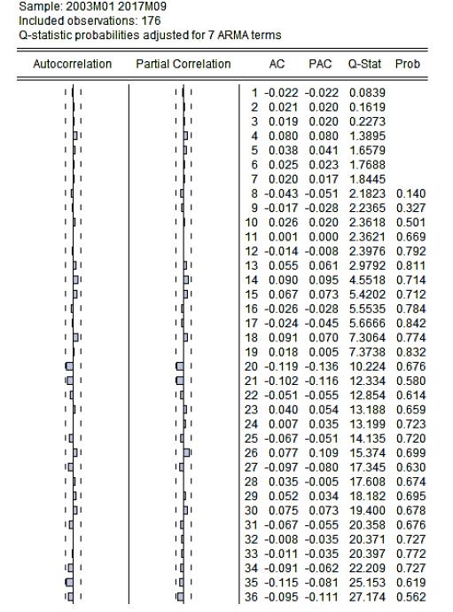
Uncorrelation. In Figure 7, the correlogram of the SARIMA (6, 1, 24) (1, 0, 1)₁₂ model analyzed by the Q statistic of Ljung-Box (Ljung & Box, 1978), shows that there is absence of autocorrelation in the error, that is, the behavior resembles that of a white noise. It is also observed that all the coefficients fall within the confidence band at 95% confidence, in addition all the p-values ​​associated with the Ljung-Box statistic for each delay (p-value) are large enough not to reject the null hypothesis that all coefficients are null. Also from Table 3 it is shown that the SARIMA (6, 1, 24) (1, 0, 1)₁₂ model, Model 1, does not present autocorrelation problems, because the Durbin-Watson (DW) statistic is around of 2 (Durbin & Watson, 1950, 1971). Consequently, the residues of the SARIMA (6, 1, 24) (1, 0, 1)₁₂ model are not correlated.

Figure 6
Residues of the SARIMA (6, 1, 24)(1, 0, 1)₁₂ model

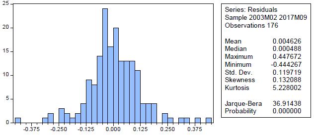
Normality. The Jarque-Bera statistic developed by Jarque & Bera (1980, 1981, 1987) is a goodness-of-fit test to verify if the study data have asymmetry or kurtosis in a normal distribution, i.e. if the residuals behave as a normal function. In Figure 8, the results of this statistic are shown, in this case the value of the probability equal to zero indicates the rejection of the hypothesis of a normal distribution. Since the value of the Jarque-Bera statistic is greater than the reference value of tables (approximately a value of 6) and the probability is less than $\alpha$=5%, the residuals of the model are not shared as a normal function. However, following the central theorem of the limit, it can be concluded that when working larger samples than the current one, it would guarantee that the errors behave as an asymptotically normal function (Laurente & Poma, 2016).

Figure 7
Correlogram of the residuals of the SARIMA (6, 1, 24)(1, 0, 1)12 model

Figure 8
Normality test of the SARIMA (6, 1, 24)(1, 0, 1)12 model

4.3 Analysis of intervention to the SARIMA (6, 1, 24)(1, 0, 1)12 model

In Figure 7 of the SARIMA (6, 1, 24) (1, 0, 1)12 model, it was proved that the residues follow a white noise behavior, that is, the residues are incorrect. On the other hand, reviewing Figure 3 and the error chart verifies the existence of two structural breaks (Chow, 1960) in February 2010 (2010m2) and February 2012 (2012m2) that was basically due to the international crisis of 2008 that affected the arrival of international tourists to Puno. Table 5 shows the estimation of the SARIMA (6, 1, 24) (1, 0, 1)12 model with intervention on both dates that represents a dummy variable with value 1 for the indicated date and 0 for its complementary, both variables are represented by the name of D2010m2 for the intervention dummy variable in the month of February 2010 and the dummy variable D2012m2 for the intervention in the month of February 2012

The results of Table 5 show the estimation of the SARIMA (6, 1, 24) (1, 0, 1)12 model previously chosen and three models that add to the indicated model the intervention in the 2010m2 and 2012m2 periods, giving as result that the best model ARIMA with intervention, is the model with intervention in 2010m2 where the variable that represents D2010m2 is statistically significant and where the model presents the lowest value of the statistics AIC (-1.255856) and SC (-1.075714) and with a value of DW = 2.066346 very close to 2, which would show the absence of autocorrelation in this model. Likewise, this SARIMA (6, 1, 24) (1, 0, 1)12 model with intervention in 2010m2 presents the statistics of AIC and SC smaller than the Model 1 because the break is being corrected in that period.

Table 5
Estimation of the SARIMA (6, 1, 24)(1, 0, 1)12 model with intervention

Variable	Coefficient	t-Statistic	AIC/SBC	DW
Model 1 (original)
constant	0.006854	2.786144	AIC = -1.179497 SC = -1.017370	2.038498
AR(1)	0.453359	3.636704
AR(3)	0.200060	2.056048
AR(6)	-0.163896	-2.390864
SAR(12)	0.980194	112.742800
MA(1)	-0.890632	-5.971538
MA(24)	-0.109057	-2.232342
SMA(12)	-0.570211	-8.484719
Model with intervention in 2010m2 and 2012m2
constant	0.007813	2.573121	AIC = -1.253463 SC = -1.055308	2.031727
AR(1)	0.448118	5.259712
AR(3)	0.189572	2.295910
AR(6)	-0.215457	-3.429775
SAR(12)	0.965115	70.765390
MA(1)	-0.871070	-9.652358
MA(24)	-0.128930	-8.000089
SMA(12)	-0.449673	-5.968413
D2010m2	-0.343730	-3.830428
D2012m2	0.148482	2.216329
Model with intervention in 2010m2
constant	0.009111	3.700238	AIC = -1.255856 SC = -1.075714	2.066346
AR(1)	0.454440	5.345148
AR(3)	0.250436	3.052563
AR(6)	-0.207885	-3.408019
SAR(12)	0.985662	144.602600
MA(1)	-0.886407	-9.171251
MA(24)	-0.113593	-7.596750
SMA(12)	-0.568242	-8.688046
D2010m2	-0.352696	-3.863401
Model with intervention in 2012m2
constant	0.005634*	1.699188	AIC = -1.186547 SC = -1.006406	2.018911
AR(1)	0.507835	3.803218
AR(3)	0.190494	2.074903
AR(6)	-0.148229	-2.005838
SAR(12)	0.977970	92.887210
MA(1)	-0.926452	-5.874378
MA(24)	-0.072634*	-1.612369
SMA(12)	-0.561978	-7.570291
D2010m2	0.192983	2.524706

• Notes: (*) means not significant at 5%. AIC and SC are the Akaike Information Criteria and the Schwarz Criteria, respectively. DW refers to the Durbin-Watson statistic of autocorrelation
• Source: The authors

Figure 9
Correlogram of the residuals of the SARIMA (6, 1, 24)(1, 0, 1)12 model with intervention in 2010m2

In Figure 9, the correlogram of the residuals of the SARIMA (6, 1, 24) (1, 0, 1)12 model with intervention in 2010m2 analyzed by the Q statistic of Ljung-Box (Ljung & Box, 1978) is shown , determines that there is an absence of autocorrelation in the residuals, that is, the behavior resembles that of a white noise because all the coefficients fall within the confidence interval at 95% confidence, in addition to all the p-values ​​associated with the statistical Ljung-Box for each delay (p-value) are large enough to not reject the null hypothesis that all coefficients are zero

Likewise, from Table 5 it is shown that the SARIMA (6, 1, 24) (1, 0, 1)12 model with intervention in 2010m2, does not present problems of autocorrelation since the Durbin-Watson (DW) statistic is found around 2. Consequently, the residues of the SARIMA (6, 1, 24) (1, 0, 1)12 model with intervention in 2010m2 are uncorrelated.

To verify if the residuals of the SARIMA (6, 1, 24) (1, 0, 1)12 model with intervention in 2010m2 behave like a normal distribution, Figure 10 shows the histogram for the Jarque-Bera statistic where its value probability is equal to zero, which indicates the rejection of the hypothesis of a normal distribution of errors since the value of the Jarque-Bera statistic is higher than the reference value of tables (approximately a value of 6) and the probability is less than $\alpha$=5%. However, following the central limit theorem, working with larger samples ensures that waste behaves as a normal function (Laurente & Poma, 2016).

Figure 10:
Normality test of the SARIMA (6, 1, 24)(1, 0, 1)12 model with intervention in 2010m2

4.4 Forecasting using the SARIMA (6, 1, 24)(1, 0, 1)12 model

After the diagnostic test performed on the SARIMA (6, 1, 24) (1, 0, 1)12 model, the forecasting of the study variable is performed (Box & Jenkins, 1976). The results are shown in Figure 11 where the variable arrivals is the original variable, arrivalsf is the forecast with the ARIMA model selected and the variable arrivalsf2010m2 is the forecast with the ARIMA model selected with intervention in 2010m2.

Figure 11
Current and forecast information with SARIMA (6, 1, 24)(1, 0, 1)12 model

Finally, using the SARIMA (6, 1, 24) (1, 0, 1)12 model, a two-year forecast of the arrival of international tourists to the Puno region is presented, which is used for administration in this sector.

Table 6
Forecasting of tourism demand using SARIMA (6, 1, 24)(1, 0, 1)12 model

	Without intervention			With intervention in 2010m2
Month-year	tourists	lower	upper	tourists	lower	upper
October 2017	31,028	23,296	38,761	30,948	23,554	38,341
November 2017	25,555	18,134	32,977	25,605	18,574	32,635
December 2017	18,019	12,493	23,546	18,030	12,855	23,205
January 2018	22,182	14,814	29,551	22,474	15,336	29,613
February 2018	19,092	12,282	25,902	19,335	12,723	25,947
March 2018	22,366	14,041	30,691	22,769	14,658	30,881
April 2018	27,166	16,854	37,478	27,991	17,863	38,119
May 2018	28,743	17,762	39,725	29,705	18,834	40,576
June 2018	25,266	15,552	34,980	26,119	16,442	35,797
July 2018	29,165	17,650	40,680	30,250	18,781	41,720
August 2018	33,763	20,497	47,029	35,247	21,965	48,530
September 2018	30,301	18,260	42,342	31,681	19,602	43,760
October 2018	32,451	18,573	46,330	33,946	19,867	48,024
November 2018	27,017	15,085	38,949	28,312	16,148	40,477
December 2018	19,434	10,761	28,107	20,306	11,466	29,146
January 2019	23,639	12,807	34,472	24,928	13,677	36,179
February 2019	20,893	11,086	30,700	22,054	11,717	32,390
March 2019	25,427	13,291	37,563	27,024	14,097	39,950
April 2019	31,291	16,091	46,491	33,590	17,226	49,955
May 2019	33,298	16,869	49,727	35,869	18,115	53,623
June 2019	29,591	14,794	44,389	31,856	15,865	47,848
July 2019	35,212	17,180	53,244	38,104	18,412	57,797
August 2019	40,583	19,635	61,530	44,167	21,315	67,020
September 2019	36,424	17,325	55,523	39,630	18,821	60,440

• Notes: (*) Bands built with ± 2S.E. 5% significance
• Source: The authors

5 CONCLUSIONS

This paper uses ARIMA modelling by Box & Jenkins (1976) for the modelling and projection of international tourism demand in the Puno region using monthly information from the years 2003 to 2017. Using the Akaike Information Criterion (AIC) and The Schwarz Criterion (SC) selected the SARIMA (6, 1, 24) (1, 0, 1)12 model as the most efficient model for the demand of international tourism in Puno. On the other hand, the Mean Absolute Percentage Error (MAPE), the percentage of measurement of the result (Z) and the normalized correlation coefficient (r) were constructed to demonstrate the efficiency of the models. The winning model of the four models proposed using these statistics is the SARIMA (6, 1, 24) (1, 0, 1)12 model with "good" forecast because it has the lowest value of the MAPE statistic equal to 16.15%. Likewise, the model presents the highest value of the percentage of the result measure (Z) equal to 16.45 and the highest value of the standardized correlation coefficient r = 0.9836. Then this winning model can be used to represent the demand for international tourism in the Puno region and its forecasting.

Finally, the results of this research can help the tourism sector in the Puno region and in Peru for proper planning and management of this very important sector in the economy.

ACKNOWLEDGEMENTS

The authors thank God for the guidance and blessing. Likewise, they thank the anonymous referees who contributed to the improvement of the work.

REFERENCES

• Akaike, H. (1974). A New Look at the Statistical Model Identification. IEEE Transactions on Automatic Control, 19(6), 716-723. https://doi.org/10.1109/TAC.1974.1100705
  » https://doi.org/10.1109/TAC.1974.1100705
• Akal, M. (2004). Forecasting Turkey’s tourism revenues by ARMAX model. Tourism Management, 25(5), 565-580. https://doi.org/10.1016/j.tourman.2003.08.001
  » https://doi.org/10.1016/j.tourman.2003.08.001
• Athanasopoulos, G., & Hyndman, R. J. (2008). Modelling and forecasting Australian domestic tourism. Tourism Management, 29 (October 2006), 19-31. https://doi.org/https://doi.org/10.1016/j.tourman.2007.04.009
  » https://doi.org/https://doi.org/10.1016/j.tourman.2007.04.009
• Baillie, R. (1996). Long Memory Processes and Fractional Integration in Econometrics. Journal of Econometrics, 73(1), 5-59. https://doi.org/10.1016/0304-4076(95)01732-1
  » https://doi.org/10.1016/0304-4076(95)01732-1
• Banco Central de Reserva del Perú - BCRP. Gerencia Central de Estudios Económicos (2018). Producto Bruto Interno por sectores productivos (millones S/ 2007). Retrieved March 26, 2019, from https://estadisticas.bcrp.gob.pe/estadisticas/series/anuales/resultados/PM05000AA/html
  » https://estadisticas.bcrp.gob.pe/estadisticas/series/anuales/resultados/PM05000AA/html
• Banco Central de Reserva del Perú - BCRP. Sucursal Puno. (2018). Síntesis de Actividad Económica, varios meses. Retrieved January 20, 2018, from http://www.bcrp.gob.pe/51-sucursales/sede-regional-puno.html
  » http://www.bcrp.gob.pe/51-sucursales/sede-regional-puno.html
• Botti, L.; Peypoch, N.; Randriamboarison, R.; & Solonandrasana, B. (2007). An Econometric Model of Tourism Demand in France. Tourismos: An International Multidisciplinary Journal of Tourism, 2(1), 115-126. Retrieved from http://mpra.ub.uni-muenchen.de/25390/
  » http://mpra.ub.uni-muenchen.de/25390/
• Box, G., & Jenkins, G. M. (1976). Time Series Analysis: forecasting and control. Oakland, California.
• CAMARA. (2018). Cámara de Comercio de Lima - Sector turismo representa 3.3% del PBI y genera 1.1 millones de empleos. Retrieved from https://www.camaralima.org.pe/repositorioaps/0/0/par/r820_2/informe economico.pdf
  » https://www.camaralima.org.pe/repositorioaps/0/0/par/r820_2/informe economico.pdf
• Cayo, N., & Apaza, A. (2017). Evaluación de la ciudad de Puno como destino turístico - Perú. Comuni@cción, 8(2), 116-124. Retrieved from http://www.scielo.org.pe/scielo.php?script=sci_arttext&pid=S2219-71682017000200005
  » http://www.scielo.org.pe/scielo.php?script=sci_arttext&pid=S2219-71682017000200005
• Chaitip, P., & Chaiboonsri, C. (2015). Forecasting with X-12-ARIMA y ARFIMA: International Tourist Arrivals to India. Annals of the University of Petroşani, Economics, 9(3), 147-162. Retrieved from http://repositorio.ana.gob.pe/handle/ANA/1564
  » http://repositorio.ana.gob.pe/handle/ANA/1564
• Chan, F., Lim, C., & McAleer, M. (2005). Modelling multivariate international tourism demand and volatility. Tourism Management, 26(3), 459-471. https://doi.org/10.1016/j.tourman.2004.02.013
  » https://doi.org/10.1016/j.tourman.2004.02.013
• Chang, C., Sriboonchitta, S., & Wiboonpongse, A. (2009). Modelling and forecasting tourism from East Asia to Thailand under temporal and spatial aggregation, Mathematics and Computers in Simulation, 79, 1730-1744. https://doi.org/10.1016/j.matcom.2008.09.006
  » https://doi.org/10.1016/j.matcom.2008.09.006
• Chokethaworn, K., Wiboonponse, A., Sriboonchitta, S., Sriboonjit, J., Chaiboonsri, C., & Chaitip, P. (2010). International Tourists’ Expenditures in Thailand: A Modelling of the ARFIMA-FIGARCH Approach. The Thailand Econometrics Society, 10(January), 85-98.
• Chow, G. (1960). Tests of Equality Between Sets of Coefficients in Two Linear Regressions. Econometrica, 28(3), 591-605. https://doi.org/10.2307/1913018
  » https://doi.org/10.2307/1913018
• Chu, F. L. (2008). A Fractionally Integrated Autoregressive Moving Average Approach to Forecasting Tourism Demand. Tourism Management, 29(1), 79-88. https://doi.org/10.1016/j.tourman.2007.04.003
  » https://doi.org/10.1016/j.tourman.2007.04.003
• CORREO. (2017). Turismo y empleo en la región Puno. Retrieved March 26, 2019, from https://diariocorreo.pe/peru/turismo-en-la-region-puno-genera-90-mil-empl-7289/
  » https://diariocorreo.pe/peru/turismo-en-la-region-puno-genera-90-mil-empl-7289/
• Coshall, J. T. (2009). Combining volatility and smoothing forecasts of UK demand for international tourism. Tourism Management, 30(4), 495-511. https://doi.org/10.1016/j.tourman.2008.10.010
  » https://doi.org/10.1016/j.tourman.2008.10.010
• Dickey, D. A., & Fuller, W. A. (1979). Distribution of the Estimators for Autoregressive Time Series With a Unit Root. Journal of the American Statistical Association, 74(366), 427-431. https://doi.org/10.2307/2286348
  » https://doi.org/10.2307/2286348
• du Preez, J., & Witt, S. F. (2003). Univariate versus multivariate time series forecasting: An application to international tourism demand. International Journal of Forecasting, 19(3), 435-451. https://doi.org/10.1016/S0169-2070(02)00057-2
  » https://doi.org/10.1016/S0169-2070(02)00057-2
• Durbin, J., & Watson, G. S. (1950). Testing for Serial Correlation in Least Squares Regression. I. Biometrika Trust, 58(1), 409-428. https://doi.org/10.2307/2332391
  » https://doi.org/10.2307/2332391
• Durbin, J., & Watson, G. S. (1971). Testing for serial correlation in least squares regression. III. Biometrika, 58(1), 1-19. https://doi.org/10.1093/biomet/58.1.1
  » https://doi.org/10.1093/biomet/58.1.1
• GESTION. (2017). Perú: Llegada de turistas por país. Retrieved March 25, 2019, from https://gestion.pe/economia/llegaran-4-8-millones-turistas-internacionales-peru-ano-10-2018-258028
  » https://gestion.pe/economia/llegaran-4-8-millones-turistas-internacionales-peru-ano-10-2018-258028
• Granger, C., & Joyeux, R. (1980). An Introduction to Long-Memory Time Series Models and Fractional Differencing. Journal of Time Series Analysis, I(1), 15-29. https://doi.org/https://doi.org/10.1111/j.1467-9892.1980.tb00297.x
  » https://doi.org/https://doi.org/10.1111/j.1467-9892.1980.tb00297.x
• Greenidge, K. (2001). Forecasting Tourism Demand An STM Approach. Annals of Tourism Research, 28(1), 98-112. https://doi.org/https://10.1016/S0160-7383(00)00010-4
  » https://doi.org/https://10.1016/S0160-7383(00)00010-4
• Hosking, J. R. M. (1981). Fractional differencing. Biometrika, 68(1), 165-176. https://doi.org/10.1093/biomet/68.1.165
  » https://doi.org/10.1093/biomet/68.1.165
• Instituto Nacional de Estadística e Informática - INEI (2018a). Pobreza por departamentos del Perú. Retrieved February 4, 2019, from https://www.inei.gob.pe/estadisticas/indice-tematico/living-conditions-and-poverty/
  » https://www.inei.gob.pe/estadisticas/indice-tematico/living-conditions-and-poverty/
• Instituto Nacional de Estadística e Informática - INEI. (2018b). Peru, PBI por departamentos según actividades económicas. Retrieved March 26, 2019, from https://www.inei.gob.pe/estadisticas/indice-tematico/pbi-de-los-departamentos-segun-actividades-economicas-9110/
  » https://www.inei.gob.pe/estadisticas/indice-tematico/pbi-de-los-departamentos-segun-actividades-economicas-9110/
• INRENA. (1995) Evaluacion de la contaminacion del lago titicaca. Retrieved from http://repositorio.ana.gob.pe/handle/ANA/1564
  » http://repositorio.ana.gob.pe/handle/ANA/1564
• Jarque, C., & Bera, A. (1980). Efficient tests for normality, homoscedasticity and serial independence of regression residuals. Economics Letters, 6(4), 255-259. https://doi.org/10.1016/0165-1765(81)90035-5
  » https://doi.org/10.1016/0165-1765(81)90035-5
• Jarque, C., & Bera, A. (1981). Efficient tests for normality, homoscedasticity and serial independence of regression residuals Monte Carlo Evidence. Journal of the American Statistical Association, 7, 313-318. https://doi.org/doi:10.1016/0165-1765(81)90035-5
  » https://doi.org/doi:10.1016/0165-1765(81)90035-5
• Jarque, C., & Bera, A. (1987). A test for Normality of observations and Regression Residuals. International Statistical Review, 55(2), 163-172. https://doi.org/10.2307/1403192
  » https://doi.org/10.2307/1403192
• Kwiatkowski, D.; Phillips, P.; Schmidt, P.; & Shin, Y. (1992). Testing the null hypothesis of stationarity against the alternative of a unit root. Journal of Econometrics, 54(1-3), 159-178. https://doi.org/10.1016/0304-4076(92)90104-Y
  » https://doi.org/10.1016/0304-4076(92)90104-Y
• Laurente, L. & Poma, R. (2016). Introducción a la teoría de las probabilidades (Primera Ed). Puno, Perú.
• Law, R., & Au, N. (1999). A neural network model to forecast Japanese demand for travel to Hong Kong. Tourism Management, 20(1), 89-97. https://doi.org/10.1016/S0261-5177(98)00094-6
  » https://doi.org/10.1016/S0261-5177(98)00094-6
• Lee, C. K.; Song, H. J.; & Mjelde, J. W. (2008). The forecasting of International Expo tourism using quantitative and qualitative techniques. Tourism Management, 29(6), 1084-1098. https://doi.org/10.1016/j.tourman.2008.02.007
  » https://doi.org/10.1016/j.tourman.2008.02.007
• Lewis, C. D. (1982). Industrial and business forecasting methods. London: Butterworths. Retrieved from http://interstat.statjournals.net/YEAR/2008/articles/0810005.pdf
  » http://interstat.statjournals.net/YEAR/2008/articles/0810005.pdf
• Lim, C., & Mcaleer, M. (1999). A seasonal analysis of Malaysian tourist arrivals to Australia. Mathematics and Computers in Simulation, 48(4), 573-583. https://doi.org/https://10.1016/S0378-4754(99)00038-5
  » https://doi.org/https://10.1016/S0378-4754(99)00038-5
• Ljung, G., & Box, G. (1978). Biometrika Trust On a Measure of Lack of Fit in Time Series Models. Biometrika, 65(2), 297-303. https://doi.org/https://doi.org/10.1093/biomet/65.2.297
  » https://doi.org/https://doi.org/10.1093/biomet/65.2.297
• Loganathan, N., & Ibrahim, Y. (2010). Forecasting International Tourism Demand in Malaysia Using Box Jenkins Sarima Application. South Asian Journal of Tourism and Heritage, 3(2), 50-60.
• Mackinnon, J. (1996). Numerical Distribution Functions for Unit Root and Cointegration Tests. Journal of Applied Econometrics, 11(6), 601-618. https://doi.org/https://doi.org/10.1002/(SICI)1099-1255(199611)11:6<601::AID-JAE417>3.0.CO;2-T
  » https://doi.org/https://doi.org/10.1002/(SICI)1099-1255(199611)11:6<601::AID-JAE417>3.0.CO;2-T
• Mamani, L. (2016). Impacto socioeconómico del turismo rural comunitario de Karina-Chucuito. Universidad Nacional del Altiplano. Retrieved from http://repositorio.unap.edu.pe/bitstream/handle/UNAP/1802/Articulo.pdf?sequence=1&isAllowed=y
  » http://repositorio.unap.edu.pe/bitstream/handle/UNAP/1802/Articulo.pdf?sequence=1&isAllowed=y
• MINCETUR. (2017a). Perú: Arribo de visitantes extranjeros a establecimientos de hospedaje, según región. Serie estadística 2003-2017. Retrieved January 17, 2018, from http://datosturismo.mincetur.gob.pe/appdatosTurismo/Content3.html
  » http://datosturismo.mincetur.gob.pe/appdatosTurismo/Content3.html
• MINCETUR. (2017b). Perú: Llegada de turistas internacionales según país de residencia permanente. Retrieved March 25, 2019, from http://datosturismo.mincetur.gob.pe/appdatosTurismo/Content1.html
  » http://datosturismo.mincetur.gob.pe/appdatosTurismo/Content1.html
• MiViaje. (2018). Descubre las islas de los uros en el lago Titicacaca - Panel fotográfico. Retrieved March 25, 2019, from https://miviaje.com/las-islas-de-los-uros-lago-titicaca/
  » https://miviaje.com/las-islas-de-los-uros-lago-titicaca/
• Nanthakumar, L., Subramaniam, T., & Kogid, M. (2012). Is “Malaysia Truly Asia”? Forecasting tourism demand from ASEAN using SARIMA approach. Tourismos, 7(1), 367-381. Retrieved from http://www.chios.aegean.gr/tourism/VOLUME_7_No1_art20.pdf
  » http://www.chios.aegean.gr/tourism/VOLUME_7_No1_art20.pdf
• Organización Mundial del Turismo - OMT. (2017). Panorama OMT del turismo internacional. Retrieved from http://www.e-unwto.org/doi/book/10.18111/9789284419043
  » http://www.e-unwto.org/doi/book/10.18111/9789284419043
• Peiris, H. (2016). A Seasonal ARIMA Model of Tourism Forecasting: The Case of Sri Lanka. Journal of Tourism, Hospitality and Sports, 22, 98-109. Retrieved from https://www.iiste.org/Journals/index.php/JTHS/article/view/33831
  » https://www.iiste.org/Journals/index.php/JTHS/article/view/33831
• Peiris, M. S., & Perera, B. J. C. (1988). On Prediction with Fractionally Differenced Arima Models. Journal of Time Series Analysis, 9(3), 215-220. https://doi.org/10.1111/j.1467-9892.1988.tb00465.x
  » https://doi.org/10.1111/j.1467-9892.1988.tb00465.x
• Phillips, P. C., & Perron, P. (1988). Testing for a unit root in time series regression. Biometrika, 75(2), 335-346. https://doi.org/10.1093/biomet/75.2.335
  » https://doi.org/10.1093/biomet/75.2.335
• Psillakis, Z., Alkiviadis, P., & Kanellopoulos, D. (2009). Low cost inferential forecasting and tourism demand in accommodation industry. Tourismos: An International Multidisciplinary Journal of Tourism, 4(2), 47-68.
• PUNO. (2017). Principales recursos turísticos em Puno. Retrieved from http://www.bcrp.gob.pe/docs/Sucursales/Puno/Puno-Atractivos.pdf
  » http://www.bcrp.gob.pe/docs/Sucursales/Puno/Puno-Atractivos.pdf
• Ray, B. K. (1993). Modeling Long Memory Processes for Optimal Long Range Prediction. Journal of Time Series Analysis, 14(5), 511-525. https://doi.org/10.1111/j.1467-9892.1993.tb00161.x
  » https://doi.org/10.1111/j.1467-9892.1993.tb00161.x
• Reisen, V. (1994). Estimation of the fractional difference parameter in the ARIMA (p,d,q) model using the smoothed periodogram. Journal of Time Series Analysis, 15(3), 335-350. https://doi.org/https://doi.org/10.1111/j.1467-9892.1994.tb00198.x
  » https://doi.org/https://doi.org/10.1111/j.1467-9892.1994.tb00198.x
• Schwarz, G. (1978). Estimating the Dimension of a Model. The Annals of Statistics, 6(2), 461-464. https://doi.org/10.1214/aos/1176344136
  » https://doi.org/10.1214/aos/1176344136
• Shareef, R., & McAleer, M. (2005). Modelling International Tourism Demand and Volatility in Small Island Tourism Economies. International Journal of Tourism Research, 7(6), 313-333. https://doi.org/10.1002/jtr.538
  » https://doi.org/10.1002/jtr.538
• Shitan, M. (2008). Time series modelling of tourist arrivals to Malaysia. Department of Mathematics, Faculty of Science, and Applied & Computational Statistics Laboratory, Institute for Mathematical Research, Universiti Putra Malaysia. Retrieved from http://interstat.statjournals.net/YEAR/2008/articles/0810005.pdf
  » http://interstat.statjournals.net/YEAR/2008/articles/0810005.pdf
• Zhou, T., Bonham, C., & Gangnes, B. (2007). Modeling the supply and demand for tourism: a fully identified VECM approach. Department of Economics and University of Hawaii Economic Reserch Organization. University of Hawaii at Manoa. Working Paper No. 07-17, July 20, 2007. https://doi.org/10.1001/archinte.165.8.854
  » https://doi.org/10.1001/archinte.165.8.854

• 1
  Peer-reviewed article.

Publication Dates

• Publication in this collection
  23 Mar 2020
• Date of issue
  Jan-Apr 2020

History

• Received
  05 Feb 2019
• Accepted
  09 Apr 2019