ABSTRACT:
RFID is an automatic contactless identification method based on radio frequency (RF). The reading process depends of the power of electromagnetic signal received by a tag. Thus an accurate characterization of RFID tags is crucial for early adopter in aerospace industry. The present study shows the preliminary approach to characterize the reading distance for UHF RFID passive tag from the low-cost application test deployment.
KEYWORDS:
RFID; Application test; Aerospace industry
INTRODUCTION
The RFID system, based on modulated backscatter process, is a wireless technology with a long history. The system has three major components: reader, antennas and tags attached at the unit under test. RFID tags can store data and modify it according to RF signal from the antennas connected to the readers. The passive tag itself can harvest power from the RF energy of the reader signal. It means that the energy to tag turn on is the key performance on the backscattered signal, where environment electromagnetic interference may significantly influence the reading process. Since current approaches to characterize UHF RFID passive tags are costly and time consuming, an economic deployment is necessary to accelerate this process. To propose such an innovative approach, an experimental study is conducted to demonstrate the feasibility of this low cost method. This paper may also be used as guideline to implement UHF RFID technology for the early adopter in the aerospace industry. It is directed to users performing application static testing of applied tags.
METHODOLOGY
The distance between UHF RFID passive tag and interrogator antenna is critical for the reading process (Nikitin et al. 2012Nikitin PV, Rao KVS, Lam S (2012) UHF RFID tag characterization: overview and state-of-the-art. Presented at: AMTA 2012. Proceedings of AMTA; Seattle, USA.). The maximum reading distance depends on the power of electromagnetic signal received by a tag (adapted from Gao et al. 2012Gao Y, Zhang Z, Lu H, Wang, H (2012) Calculation of read distance in passive backscatter RFID systems and application. Journal of System and Management Sciences 2(1):40-49.) (Fig. 1).
Luh and Liu (2013)Luh YP, Liu YC (2013) Measurement of effective reading distance of UHF RFID passive tags. Modern Mechanical Engineering 3(3):115-120. doi: 10.4236/mme.2013.33016
https://doi.org/10.4236/mme.2013.33016...
define this power as necessary to turn on the RFID tag (Pturn-on). To determine methodologically the value of (Pturn-on), EPC Global publishes the Application Static Test as industrial standard. Originally, this Application Test was methodologically consolidated in three phases (Fig. 2):
Response Test structure for the experimental component (adapted from EPC Global 2008EPC Global (2008) Static test method [S.l]; [accessed 2016 April 10]. https://www.gs1.org/epcglobal/
https://www.gs1.org/epcglobal/... and from Puleston and Foster 2006Puleston DJ, Forster I (2005) The test pyramid: a framework for consistent evaluation of RFID tags from design and manufacture to end use. Avery Dennison Press Release.).
PHASE 1: RF ENVIRONMENT INTERFERENCE
RF Interference in the environment is mostly guided to the aspects related to the places where the tests will take place (open or closed area), as well as to the attentions and minimum measures to be taken in each one of the scenarios (Griffin and Durgin 2009Griffin JD, Durgin GD (2009) Complete link budgets for backscatter-radio and RFID systems. IEEE Antennas and Propagation Maganize 51(2):11-25. doi: 10.1109/MAP.2009.5162013
https://doi.org/10.1109/MAP.2009.5162013...
). Ideally, it should be chosen application tests in closed areas (anechoic chamber), but in this case, they could not be performed for economic reasons and purpose of this paper. As per the EPC Policy, the minimum necessary area, characteristic of open areas, is 2,440 mm × 2,440 mm × 3,660 mm. Environment interferences above -60 dBm jeopardize the test in both open or closed areas.
Basic directive of noise measure in open area following EPC Global Policy
The maximum noise level allowed for open area is -60dBm, measured with frequency range between 0.5 and 3.0 GHz, band resolution (RBW) of 100 kHz and span of 50 MHz, during one reading hour (EPC Global 2008EPC Global (2008) Static test method [S.l]; [accessed 2016 April 10]. https://www.gs1.org/epcglobal/
https://www.gs1.org/epcglobal/...
). For example, this measurement can be made with Aaronia HF 2025E portable analyzer (Fig. 3).
Environment conditions
The required temperature and humidity conditions for the environment (open or closed areas) are described in Table (EPC Global 2008EPC Global (2008) Static test method [S.l]; [accessed 2016 April 10]. https://www.gs1.org/epcglobal/
https://www.gs1.org/epcglobal/...
).
PHASE 2: CORRECTION FACTOR DEFINITION
Correction Factor is used to define the UHF RFID tags operation sensitivity (Tag Turn On), being attached to units under test (UUT). This phase is subdivided in: Theoretical Maximum Power in the Reference Point; and Power correction factor calculus.
Theoretical Maximum Power in the Reference Point
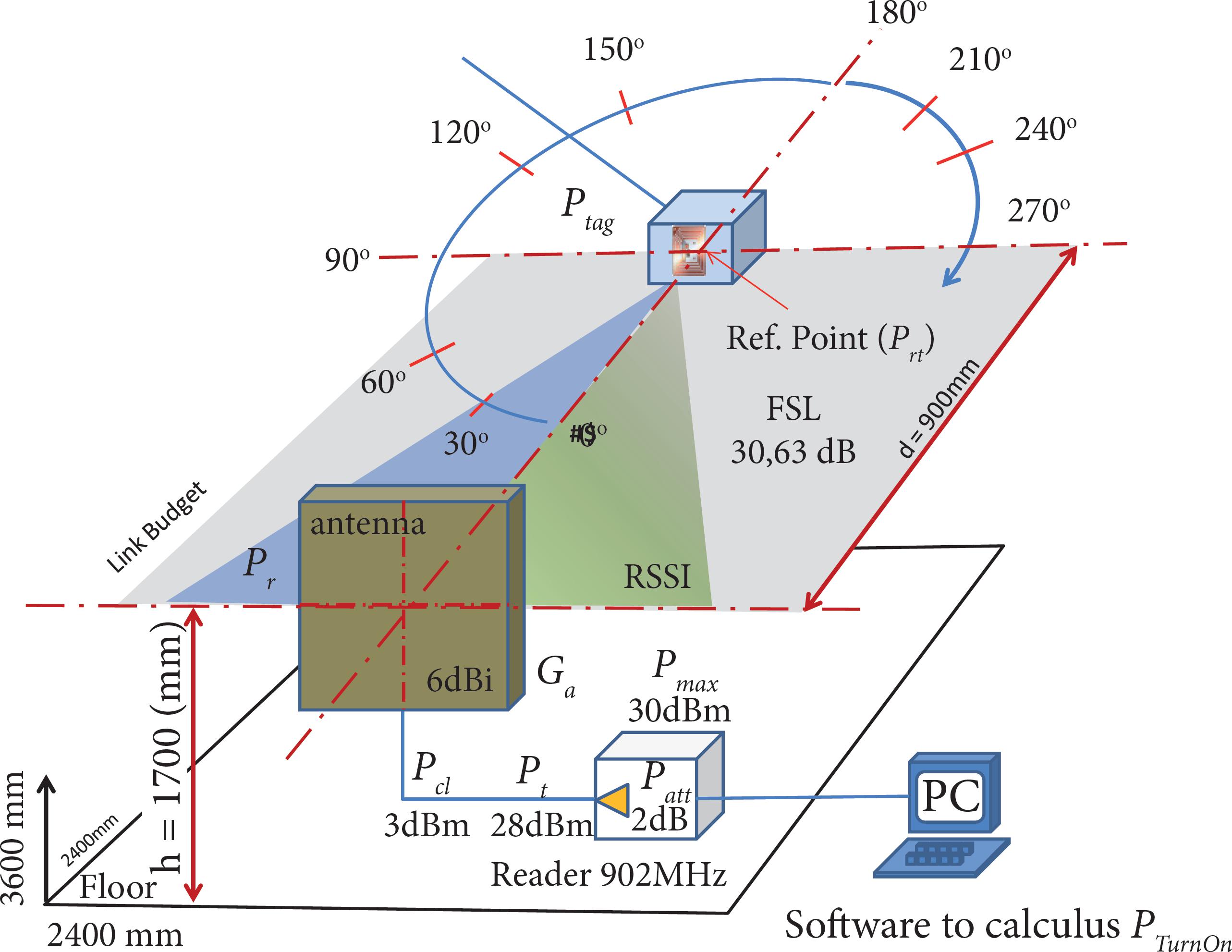
Proposed by EPC, the measure is made from a known dipole antenna (e.g., A.H. Systems, Model FCC-4), joining a power measure system (e.g., Spectrum Analyzer) in a closed ambient (anechoic chamber). Since we could not have access to an anechoic chamber or to a calibrated dipole antenna, this paper proposes an alternative way to find the power at the reference point in an open area. Figure 4 resumes the proposal (adapted from EPC Global 2008EPC Global (2008) Static test method [S.l]; [accessed 2016 April 10]. https://www.gs1.org/epcglobal/
https://www.gs1.org/epcglobal/...
) (adapted from Puleston and Foster 2006Puleston DJ, Forster I (2005) The test pyramid: a framework for consistent evaluation of RFID tags from design and manufacture to end use. Avery Dennison Press Release.):
According to Fig. 3, the theoretical maximum power (Prt) at the Reference Point can be calculated with known factors of this system. The first factor to be defined is the loss of free space propagation (FSL). The second factor is the losses in cables and connectors of the circuit, which is directly applied in the table calculus of the Prt.
The propagation loss (FSL) can be calculated from Eq. 1 (Nikitin et al. 2012Nikitin PV, Rao KVS, Lam S (2012) UHF RFID tag characterization: overview and state-of-the-art. Presented at: AMTA 2012. Proceedings of AMTA; Seattle, USA.):
where: d = distance in reading meters between the broadcasting antenna and the RFID tag; f = frequency in MHz to be tested.
Based on FSL (Eq. 1) and on theoretical loss in cables and connectors, it is possible to calculate the Theoretical Maximum Power (Prt) at the Reference Point (Table 2).
From the same rationale, Table 3 presents the (Prt) for three main frequencies used in UHF RFID passive tags:
There is an assumption that the reflections in the reference point do not jeopardize the tests results (height = 1700 mm above the floor), once the point was located in the center of the established dimensions for open area (minimize reflections from the walls and ceiling). Besides, the measured local noise was around -66.00 dBm for the frequencies of 902, 915 and 928 MHz, within the established limit in the EPC policy (< -60 dBm).
Once these values are defined, it's not necessary to recalculate them for new tests. This is valid if the setup reader/antenna/cable and open area are the same. Interference level always measured to be complied with EPC standards.
Power Correction Factor Calculus
Based on Table 2, it was created a reference table in order to find the theoretical Power Correction Factor for each frequency range (Table 4).
With the results on Table 4, it is possible to define the PturnOn in the next phase.
PHASE 3: DEFINE TAG TURN ON POWER
Theoretical Offset Calculus
Since an external attenuator was not utilized in the setup (Fig. 4), a theoretical attenuator (offset) could adopt and apply over reader power. According to Luh and Liu (2013)Luh YP, Liu YC (2013) Measurement of effective reading distance of UHF RFID passive tags. Modern Mechanical Engineering 3(3):115-120. doi: 10.4236/mme.2013.33016
https://doi.org/10.4236/mme.2013.33016...
and Nikitin and Rao (2008)Nikitin PV, Rao KVS (2008) Antennas and Propagation in UHF RFID Systems. Presented at: IEEE International Conference on RFID 2008. Proceedings of IEEE International Conference on RFID; Las Vegas, USA. p. 277-288. doi: 10.1109/RFID.2008.4519368
https://doi.org/10.1109/RFID.2008.451936...
(Eq. 2),
Considering initially tag sensitivity as Ptag = 0 (Fig. 1), Eq. 3 allows the definition of a theoretical offset (Patt):
where: reader Maximum Power Broadcasted (Pt) (e.g., 30.00 dBm); loss in connectors and cable (Pcl) (e.g., 3.00 dB); broadcasting Antenna Gain (Ga) (e.g. 6.00 dBi); loss in Free Space Propagation (FSL) (e.g., 30.75 dB for 0.9 m).
With the data provided as examples in Eq. 3, it is possible to calculate the attenuation to be inserted in the system (Eq. 4):
It means that the reader maximum power (Pti would initially be (Eq. 5):
In this case, the initial setup for the initial reader maximum power (Pti) would not be above 30.00 dBm, but 27.75 dBm (~ 28.00 dBm). From this value, the power would be attenuated in steps of 1.00 dBm directly in the reader, until the reading response stays below 50% of interrogations, following the EPC Global policy. Consequently, the calculated tag sensitivity, Ptag, would be reported for analysis effect between 0 dBm and -19.00 dBm. In real life, this covers almost all the RFID tags available in the market. The Offset should be used only when there is a need, not characterizing a mandatory procedure.
Tag Turn on Power Calculus
Based on the calculations and on the provided values in previous examples, consider the theoretical setup below (Fig. 5). Table 5 presents the final calculus of Tag Turn on Power in open area, and Table 6 summarizes all results.
Remark: The scope of this paper limited the test only in the 0° angle (Fig. 5).
EXPERIMENTAL STUDY AND RESULTS
The RFID system is designed to achieve better inventory control, responsive replenishment and improve its quality of service (Zhu et al. 2012Zhu X, Mukhopadhyay SK, Kurata H (2012) A review of RFID technology and its managerial applications in different industries. Journal of Egineering and Technology Management 29(1):152-167. doi: 10.1016/j.jengtecman.2011.09.011
https://doi.org/10.1016/j.jengtecman.201...
). In the aerospace industry RFID technology are used to track and identify items as part of trading partner programs, MRO and internal material management. To achieve this purpose it is important to select correctly the RFID tag. In the real world, temperature, dust, metal, chemical products (and many others) are omnipresent elements in all sectors of industry and particularly in Aerospace (Su et al. 2010Su Z, Cheung S, Chu KT (2010) Investigation of radio link budget for UHF RFID systems. Presented at: IEEE International Conference on RFID - Technology And Applications 2010. Proceedings of IEEE International Conference on RFID - Technology And Applications; Guangzhou, China. p. 164-169. doi: http://10.1109/RFID-TA.2010.5529938
http://10.1109/RFID-TA.2010.5529938...
). These elements are disturbing factors for wireless technologies including RFID (Wang et al. 2009Wang HG, Pei CX, Zheng F (2009) Performance analysis and test for passive RFID system at UHF band. The Journal of China Universities of Pots and Telecommunications 16(6):49-56. doi: 10.1016/S1005-8885(08)60288-5
https://doi.org/10.1016/S1005-8885(08)60...
). In this experimental study, the effective reading distance of a tag was characterized by the setup shown on Fig. 5, but all disturbing factors from environment were inconsiderate at this moment. Figure 6 presents the setup developed in the laboratory to validate the Application Static Test methodology.
In this setup (Fig. 6), the tag was oriented to match the reader antenna polarization. Table 7 presents a result with the simplified characterization process.
Comparison between tag Manufacturer information and Simplified Static Test developed (Tag Turn on).
Converting Tag turn on to maximum reading distance by the software under development (Table 8).
Comparison between tag Manufacturer information and Simplified Static Test results (Max Reading Distance).
It is possible to observe that the best tag sensitivity value (-3.23 dBm - Table 7) corresponds to the best tag range 2.26 m - Table 8).
CONCLUSIONS
The stat-of-the-art approach is to position the RFID tag from interrogator antenna in anechoic chamber and to attenuate the signal until backscattering drop from 50% reading tax. However, such approach is costly and time consuming. This preliminary study proposes a new approach to accelerate the characterization process for UHF RFID Passive Tags for early adopter in the Aerospace industry. The results presented are satisfactory considering the similarity with those provided by the Xerafy manufacturer to reading on free space. In this way, it is possible to extend the test to other components using the same tag manufacturer or other, thus verifying the result for each application. In addition, tests with other angles may present new results for the same component (see Fig. 5). This is important considering the process where the component will be read in the future.
REFERENCES
- EPC Global (2008) Static test method [S.l]; [accessed 2016 April 10]. https://www.gs1.org/epcglobal/
» https://www.gs1.org/epcglobal/ - Gao Y, Zhang Z, Lu H, Wang, H (2012) Calculation of read distance in passive backscatter RFID systems and application. Journal of System and Management Sciences 2(1):40-49.
- Griffin JD, Durgin GD (2009) Complete link budgets for backscatter-radio and RFID systems. IEEE Antennas and Propagation Maganize 51(2):11-25. doi: 10.1109/MAP.2009.5162013
» https://doi.org/10.1109/MAP.2009.5162013 - Luh YP, Liu YC (2013) Measurement of effective reading distance of UHF RFID passive tags. Modern Mechanical Engineering 3(3):115-120. doi: 10.4236/mme.2013.33016
» https://doi.org/10.4236/mme.2013.33016 - Nikitin PV, Rao KVS (2008) Antennas and Propagation in UHF RFID Systems. Presented at: IEEE International Conference on RFID 2008. Proceedings of IEEE International Conference on RFID; Las Vegas, USA. p. 277-288. doi: 10.1109/RFID.2008.4519368
» https://doi.org/10.1109/RFID.2008.4519368 - Nikitin PV, Rao KVS, Lam S (2012) UHF RFID tag characterization: overview and state-of-the-art. Presented at: AMTA 2012. Proceedings of AMTA; Seattle, USA.
- Puleston DJ, Forster I (2005) The test pyramid: a framework for consistent evaluation of RFID tags from design and manufacture to end use. Avery Dennison Press Release.
- Su Z, Cheung S, Chu KT (2010) Investigation of radio link budget for UHF RFID systems. Presented at: IEEE International Conference on RFID - Technology And Applications 2010. Proceedings of IEEE International Conference on RFID - Technology And Applications; Guangzhou, China. p. 164-169. doi: http://10.1109/RFID-TA.2010.5529938
» http://10.1109/RFID-TA.2010.5529938 - Xerafy (2015) Dash-in XS; [accessed 2016 April 10] http://www.xerafy.com/en/catalogue/product/dash-in-xs/2
» http://www.xerafy.com/en/catalogue/product/dash-in-xs/2 - Wang HG, Pei CX, Zheng F (2009) Performance analysis and test for passive RFID system at UHF band. The Journal of China Universities of Pots and Telecommunications 16(6):49-56. doi: 10.1016/S1005-8885(08)60288-5
» https://doi.org/10.1016/S1005-8885(08)60288-5 - Zhu X, Mukhopadhyay SK, Kurata H (2012) A review of RFID technology and its managerial applications in different industries. Journal of Egineering and Technology Management 29(1):152-167. doi: 10.1016/j.jengtecman.2011.09.011
» https://doi.org/10.1016/j.jengtecman.2011.09.011
Edited by
Publication Dates
-
Publication in this collection
2018
History
-
Received
12 May 2016 -
Accepted
08 Aug 2017