Synthesis of Sparse Arrays Based On CIGA (Convex Improved Genetic Algorithm)

Abstract

In this paper, a novel hybrid algorithm on beam pattern synthesis of sparse arrays is proposed, which aims at minimizing the peak sidelobe level (PSLL). Sparse arrays can provide higher spatial resolution and relatively lower sidelobe than general arrays, but it is necessary to solve the multi-constraint problem of nonconvex nonlinear. Thus, we propose a Convex Improved Genetic Algorithm (CIGA) that can adjust the positions and the excitation coefficients of arrays to achieve the minimum PSLL. The CIGA is an effective two-step approach to the synthesis of sparse array. Firstly, Improved Genetic Algorithm is proposed, which is suitable for beam pattern synthesis of sparse arrays. The Improved Genetic Algorithm is adopted to adjust the positions of arrays to achieve the local optimum PSLL, and then convex optimization method is used to calculate the excitation coefficients in expectation of reaching the minimum PSLL. Simulation results show that the PSLL obtained by CIGA is about 5dB better than the published methods in sparse linear arrays and prove that the CIGA is superior to the published methods.

Index Terms
Sparse arrays; beam pattern synthesis; peak sidelobe level (PSLL); convex optimization

I. INTRODUCTION

Nowadays, antenna arrays can be widely applied to a system including radar, radio astronomy and satellite communication system. Synthesis of antenna arrays has been researched for several decades. Different from synthesis of single-antenna, synthesis of antenna arrays can be considered as a multi-constraint optimization problem, which requires more advanced optimization methods [¹]. In many practical applications, antenna arrays often require low sidelobe. For example, the PSLL of uniform Substrate Integrated Waveguide slot antenna arrays is close to –13.60dB, but in common radar system, the lower PSLL is often required [²]. Therefore, it is necessary to research an effective method to depress the PSLL of antenna arrays.

Analyzing the expression of the array factor, we find that the element positions and amplitude and phase of the excitation coefficients are the main factors affecting the radiation pattern of antenna arrays. Generally, there are two categories of array layouts for unequally spaced arrays: Thinned Arrays, where selecting the appropriate array elements from the equally spaced arrays [³]; sparse arrays, where the array elements can be arranged arbitrarily within the array aperture [⁴]. It is clear that the former reduce the degree of freedom of the optimization process, and cannot get the minimum PSLL, so the former is limited in scope of application. The latter can make the PSLL as low as possible, but algorithm is relatively complex [⁵].

In the past few years, many synthesis methods of antenna arrays have been developed. The methods of antenna arrays synthesis based on stochastic optimization algorithm are proved effectively, such as genetic algorithm (GA) [⁶,⁷], differential evolution (DE) [⁸], particle swarm optimization (PSO) [⁹], invasive weed optimization [¹⁰] and cuckoo search algorithm[¹¹], dynamic parameters differential evolution algorithm (DPDE) [¹²], improved chicken swarm optimization [¹³]. Such methods are effective for optimizing amplitude and phase of the excitation coefficients of the equally spaced arrays or optimizing the element positions with the uniform excitation coefficients, but it cannot achieve the truly minimum PSLL when both the excitation coefficients and the element positions are considered. An effective method has been proposed in [¹⁴], which can consider both the excitation coefficients and the element positions simultaneously, but only the intelligent optimization algorithm is used, which leads to the result without good stability. Some other synthesis techniques are much more efficient than the stochastic optimization algorithms, such as compressive sensing based synthesis approaches in [¹⁵] and [¹⁶], bayesian compressive sensing based synthesis approaches in [¹⁷] and [¹⁸], the matrix pencil methods in [¹⁹] and [²⁰], two step approach (TSA) [²¹]. However, these methods reduce the degree of freedom of antenna arrays, leading to a local optimal solution eventually. Recently, a better arrays synthesis method can be achieved while improving the computational efficiency, utilizing a global optimization algorithm that applies the density tapper technology [²²].

In this paper, inspired by the idea that presented in [²²], the novel convex improved genetic algorithm (CIGA) is proposed for the non-uniform excitation coefficients arrays that the array elements can be arranged arbitrarily within the array aperture. Firstly, the uniform excitation coefficients are set under the condition of unchanged aperture of the array to obtain the optimal array layout. Then, this problem is transformed into a convex optimization problem that can be processed by Interior Point Method, Gradient Descent Method, or the like. Finally, the minimum PSLL can be obtained and experimental results verify the effectiveness and outperformance of the proposed method.

II. Problem Formulation

A. Array factor

In the following discussion, we will consider the case of planar arrays because linear arrays can be regarded as a special planar array. For example, there is an array of N radiation elements and the array factor AF of planar arrays can be mathematically formulated as follows [²³]:

(1) $$AF(u,v)={\displaystyle \sum _{n=1}^N{w}_n{e}^{j\beta (x_{n}u+y_{n}v)}}$$

where (x_n, y_n) is the coordinate of the nth array element, w_n is a complex variable that represents the excitation coefficient of the nth array element. β = 2π/λ is the free space wavenumber, λ is the wavelength. u = sin θ cos ϕ – sin θ₀ cos ϕ₀ and v = sin θ sin ϕ – sin θ₀ sin ϕ₀ (θ ∊ (0, π), ϕ ∊ (0, 2π)). θ₀ and ϕ₀ are the main beam pointing direction. The geometry and notation of planar arrays are demonstrated in Fig. 1.

Fig. 1
geometry and notation of planar arrays.

The radiation pattern of planar arrays can be expressed as [²⁴]:

(2) $$P_{{\Omega }_{1,}{\Omega }_2}(u,v)={\left|AF(u,v)\right|}^2$$

where Ω₁ and Ω₂ represent the main lobe region and sidelobe region, respectively.

B. Formulation description, NP-Hardness and convex optimization

1) Problem description

The purpose of this paper is to find an optimal set of the positions and amplitude and phase of the excitation coefficients, so that the PSLL is as low as possible. Thus, this optimization problem can be described as:

(3a) $$\min \Upsilon \text{(}w,x,y\text{)=10lg}\frac{{\max }_{(\theta ,\varphi )\in {\Omega }_2}P(u,v)}{{\max }_{(\theta ,\varphi )\in {\Omega }_1}P(u,v)}$$

(3b) $$s.t.0<\left|w_n\right|\le 1$$

(3c) $$P(u_0,v_0)=1$$

(3d) $$x_N=L_x,y_N=L_y$$

(3e) $$0\le x_n<L_x,0\le y_n<L_y,n=1,2,\cdots ,N-1$$

where (θ, ϕ) represents the visible area, w = [w₁, w₂, L, w_N] is the excitation coefficients vector, x = [x₁, x₂, L, x_N]^T and y = [y₁, y₂, L, y_N]^T are the coordinate vectors. Constraint (3b) gives the ranges of excitation coefficient of the nth element. Constraint (3d) and (3e) indicate the size of the array aperture. Constraint (3c) (u₀ = sin θ₀ cos ϕ₀, v₀ = sin θ₀ sin ϕ₀ (θ₀, ϕ₀) ∊Ω₁) represents normalized main beam pointing and it is actually the maximum value of the main lobe level, so the denominator of Eq. (3a) can be regard as fixed value 1.

2) NP-Hardness and convex optimization

To prove that this optimization problem is a NP-hard, we first simplify the continuous optimization problem to the discrete optimization problem. Take a 10-element linear arrays as an example and set λ = 1. The set of array elements spacing is S = {0.51, 0.52, 0.53, 0.54, 0.55, 0.56, 0.57, 0.58, 0.59}, the set of excitation coefficient of the antenna elements is C = {0.1, 0.2, 0.3, 0.4, 0.5, 0.6, 0.7, 0.8, 0.9, 1.0}. The coordinates of each array elements can obtained by the set of array elements spacing S, each array elements could have an excitation coefficient from the set C, so this problem is a combinatorial optimization problem. In general, the combinatorial optimization problem can be represented by three parameters (D, F, f), where D represents the domain of the decision variable, it is actually the Constraint (3b) and (3d). F represents the cost function, which is the Eq. (3a). f represents the region of feasible solution. Thus, the formulated problem in Eqs. (3a) - (3e) is NP-hard. When the element positions is fixed, we can convert cost function γ(w, x, y) into γ(w). γ(w) is obviously a convex function. So the optimization problem is transformed intow a convex optimization problem when the element positions are determined.

III. Problem Solution

The proposed algorithm is divided into two steps, the details will be described in this section.

Step A. optimal positions

Under the condition of the uniform excitation coefficients, the problem is transformed into a single objective optimization problem for finding the optimal positions. Since the problem of finding the optimal positions is non-linear and non-convex, an intelligent optimization algorithm is usually used. In this paper, the optimal array element positions are solved by the IGA. The optimization model can be expressed as:

(4a) $$\min \Upsilon \text{(}x,y\text{)=10lg}\frac{{\max }_{(\theta ,\varphi )\in {\Omega }_2}P(u,v)}{{\max }_{(\theta ,\varphi )\in {\Omega }_1}P(u,v)}$$

(4b) $$s.t.P(u_0,v_0)=1$$

(4c) $$x_N=L_x,y_N=L_y$$

(4d) $$0\le y_n<L_x\text{,\hspace{0.17em}}0\le y_n<L_y,n=1,2,\cdots N-1$$

The process of the IGA is as follows:

1. Initialization parameters: The population size is set as NP, iteration number is set as G and the number of elements of the array is set to N. Each individual is represented as (x_i,g, y_i,g) i = 1,2,L, NP, g = 1,2,…G, x_i,g and y_i,g are random numbers that satisfy the constraint (4d).

2. Selection: The traditional roulette method is adopted, and the possibility of the children reservation are determined by size of the individual fitness. The fitness of the ith is f_i, the probability of selection SP can be expressed as:

   (5) $$S{P}_i=\frac{f_i}{{\displaystyle \sum _{i=1}^{NP}{f}_i}},i=1,2,\dots ,NP$$

3. Crossover: Firstly, the population is divided into a set of odd number of individuals and a set of even number of individuals. The integers in [¹, N] are randomly selected as the intersection points, and then the crossover is carried out according to the crossover probability, and the respective partial genes are exchanged at the intersection point of the paired individuals and forming a pair of new individuals. To achieve a better optimizing performance than the traditional GA, we introduce adaptive crossover probability P_c:

   (6) $$P_c=k_1\times \frac{\arcsin (f_{ave}/f_{\max })-{\xi }_1}{\pi /2}$$

   where f_ave and f_max represent the average fitness and the maximum fitness, respectively. In this way, P_c can change dynamically during optimization process. In order to preserve the characteristics of genetic algorithm and prevent it from becoming the general stochastic search algorithm, the constants k₁ and ζ₁ are introduced. According to experience, k₁ is 1.9 and ζ₁ is 0.5.

4. Mutation: The mutation probability P_m of an individual is a parameter as important as the crossover probability P_c. A smaller fitness leads to a higher mutation probability. P_m is computed by

   (7) $$P_m=k_2\times \left(1-\frac{\arcsin (f_{ave}/f_{\max })-{\xi }_2}{\pi /2}\right)$$

where the constants k₂ and ζ₂ are introduced to prevent the maximum mutation probability P_m from exceeding 0.1, according to experience, we set k₂ = 0.18 and ζ₂ = 0.4.

Step B. optimal excitation coefficients

After the optimal positions of the array elements are obtained, the problem can be transformed into a convex optimization problem, and the optimal excitation coefficients are obtained by using the traditional convex optimization methods (Interior Point Method, Newton-Decline Method and so on). The optimization model can be expressed as:

(8a) $$\min \Upsilon \text{(}w\text{)=10lg}\frac{{\max }_{(\theta ,\varphi )\in {\Omega }_2}P(u,v)}{{\max }_{(\theta ,\varphi )\in {\Omega }_1}P(u,v)}$$

(8b) $$s.t.0<\left|w_n\right|\le 1$$

(8c) $$P(u_0,v_0)=1$$

IV. SIMULATION RESULTS

In this part, some simulation experiments are carried out to verify the effectiveness and the advantages of the CIGA. The proposed CIGA algorithm is evaluated by Matlab. The CPU used for simulation is CORE i7, the RAM is 4G and the operation system is Windows 10. First, by comparing with GA, the effectiveness of the algorithm proposed in the step A is explained. Second, the PSLL of the power patterns of the linear array antennas scenario and the planar array antennas scenario are optimized by CIGA.

A. Linear array antennas scenario

We consider a N-element linear sparse arrays, shown in Fig. 2.

Fig. 2
N-element linear sparse arrays.

To explain the effectiveness of the algorithm proposed in the step A, we compare the performance of the IGA with that of GA. We consider a linear sparse arrays with L = 98.5 λ and N = 152. Table I summarizes the comparative results between GA and the IGA, after 50 independent runs, the worst-case PSLL, the best-case PSLL and the average PSLL obtained by the IGA are better than that of GA. In addition, the CPU running time obtained by the IGA are shorter than that of GA. Fig. 3 shows the convergence during the optimization process obtained by GA and the IGA.

Table I
Comparative results

N	152
Method	GA	IGA
Population size	50	30
Number of generations	100	100
Worst-case PSLL(dB)	−16.20	−16.27
Best-case PSLL(dB)	−17.23	−17.50
Average PSLL(dB)	−16.66	−16.80
Runtime(s)	91.32	55.20

Fig. 3
Convergence during the optimization process obtained by GA and IGA.

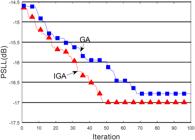
It can be seen that the accuracy, the convergence and the CPU running time can be effectively improved by using IGA. Note that the IGA is the first step of CIGA, the IGA is used to achieve the optimum array geometry that must meet the minimum spacing constraint. Once the optimum array geometry has been defined, we could calculate their excitation coefficients by means of convex programming, such as the CVX and SeDumi.

In order to illustrate the superiority of the proposed algorithm in this paper, the CIGA is compared with Dynamic parameters differential evolution algorithm (DPDE) [¹²], Two Step Approach (TSA) [²¹] and Improved Genetic Algorithm [¹⁴]. The minimum elements spacing d_c is 0.5λ, which is the same as that of the reference algorithms. The element coordinate vector x = [x₁, x₂,L, x_N]^T can be divided into two vectors.

(9) $$x=v+m$$

where m = [0, d_c, 2d_c, L, (N – 1)d_c]^T represents the minimum elements spacing vector and v represents the positions information of the array elements that need to be optimized.

Example A: In order to make comparison with the literature, the CIGA is set the same array parameters as provided in [¹²], L = 98.5λ and N = 152. Fig. 4(a) shows the normalized radiation pattern of the best solution obtained by the CIGA. Fig. 4(b) depicts the PSLL after that the proposed method runs 50 times. The best PSLL is −29.02dB and the mean PSLL is −28.55dB, as Table II shows, which is about 5dB better than the PSLL obtained by these algorithms mentioned in [¹²].

Table II
The psll obtained by different algorithms for 152-element arrays

Algorithm	Best-case PSLL(dB)	Average PSLL(dB)
CIGA	−29.2	−28.55
DPDE[12]	−24.14	−23.76
NBDE	−21.15	−20.78
Boolean PSO	−20.86	−20.20
BGA	−19.08	−18.17

Fig. 4
(a) Normalized radiation pattern. (b) The PSLL of runs 50 times.

Example B: In order to make fair comparison with the TSA [²¹], further researches of linear sparse arrays (LSA) with L = 9.7440λ, N = 17 and L = 21.9960λ, N = 37 are carried out to examine the performance of the CIGA. In 100 independent tests, the optimal positions and the optimal excitation coefficients of 17-element linear sparse arrays are depicted in Table IV, Table V. The CIGA has achieved a best PSLL of −23.14dB for the 17-element arrays and −24.76dB for the 37-element arrays, as Table III depicts, which are better than those algorithms mentioned by [²¹]. The pattern of 17-element arrays and 37-element arrays are plotted in Fig. 5(a) and Fig. 5(b).

Table III
The PSLL obtained by different algorithms for 17-element and 37-element arrays

Algorithm	PSLL(dB)
	17-element	37-element
CIGA	−23.14	−24.76
MGA	−19.80	−20.56
SaDE	−19.90	−20.94
TSA [21]	−19.90	−21.03

Fig. 5
(a) 17-element arrays radiation pattern. (b) 37-element arrays radiation pattern

Table IV
17-Element Positions (λ) Obtained by the CIGA

17-element
n	Position	n	Position
1	0	10	5.3235
2	0.5552	11	5.8614
3	1.5334	12	6.3805
4	2.1536	13	6.9213
5	2.7358	14	7.4869
6	3.2788	15	8.1790
7	3.7794	16	9.0014
8	4.2862	17	9.7440
9	4.8068

Table V
Optimal excitation Coefficients of 17-element Arrays

17-element
n	Excit	n	Excit	n	Excit
1	0.0358+0.0010i	7	0.0605+0.0016i	13	0.0587+0.0016i
2	0.0474+0.0013i	8	0.0691+0.0019i	14	0.0591+0.0016i
3	0.0616+0.0017i	9	0.0653+0.0018i	15	0.0616+0.0017i
4	0.0512+0.0014i	10	0.0723+0.0020i	16	0.0612+0.0016i
5	0.0639+0.0017i	11	0.0656+0.0018i	17	0.0424+0.0011i
6	0.0590+0.0016i	12	0.0649+0.0018i

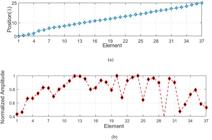
Example C: In this example, we consider a linear sparse arrays with L = 25λ and N = 37 and the selected parameters are the same as those in [¹⁴]. Fig. 6(a) and Fig. 6(b) display the optimal positions and amplitude of the normalized excitation coefficients. As exhibited in Fig. 7, the best PSLL of the CIGA is −23.69dB, which is about 1.2 dB better than the best result of the method in [¹⁴].

Fig. 6
(a) Positions obtained using the CIGA. (b) Normalized amplitude obtained using the CIGA.

Fig. 7
37-element arrays radiation pattern from the CIGA.

B. Planar array antennas scenario

We consider a sparse planar array with 100 radiation elements in the range of 10λ × 10λ. The optimal array layout obtained by the CIGA is shown in Fig. 8. Fig. 9(a) clearly shows the radiation pattern of the planar antenna arrays obtained by the CIGA, for a more intuitive view of the PSLL of the array pattern, power mask is drawn at the PSLL. It is clearly shows that the CIGA has achieved the best PSLL of −13.30dB, which is better than that of improved chicken swarm optimization [¹³]. Fig. 9(b) shows the top view of radiation pattern of the planar antenna arrays.

Fig. 8
Planar array layout obtained by the CIGA. (N = 100).

Fig. 9
(a) Radiation pattern of planar antenna arrays. (b) The top view of radiation pattern. (N = 100).

In some special applications, more antenna elements are often required to obtain the desired the radiation pattern. Thus, planar antenna arrays with 400 radiation elements are applied to validate the performance of the proposed CIGA for the large-scale arrays. In Fig. 10(a), the results show that the PSLL is −14.65dB, which is lower than that of the improved chicken swarm optimization proposed in [¹³]. Fig. 10(b) shows the top view of radiation pattern of the planar antenna arrays. Obviously, the energy is more concentrated than that of the 100 elements planar antenna arrays.

Fig. 10
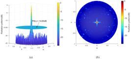
(a) Radiation pattern of planar antenna arrays. (b) The top view of radiation pattern. (N = 400).

V. Conclusion

To solve the nonconvex nonlinear problem in the synthesis of sparse arrays, a novel hybrid algorithm is proposed in this paper. The proposed algorithm has the advantages of the IGA and the convex optimization method. The PSLL obtained by the CIGA can get 20% reduction of that of the swarm intelligent optimization algorithms [¹²]-[¹⁴], [²¹] in sparse linear arrays. In sparse planar arrays, the PSLL obtained by the CIGA can get 7% reduction of these methods mentioned in [¹³]. In addition, it can be seen from the results of multiple independent runs that the proposed algorithm has good stability. Whether a linear arrays with a small number of elements or a large-scale planar arrays, the proposed CIGA provides better performance than the other published methods.

ACKNOWLEDGMENT

This work was supported by the National Natural Science Foundation of China (Grant No. 51877151), Tianjin Municipal Natural Science Foundation (Grant No. 18JCZDJC99900) and the Program for Innovative Research Team in University of Tianjin (Grant No. TD13-5040).

References

• ^[1]
  Darvish and A. Ebrahimzadeh, “Improved Fruit-Fly Optimization Algorithm and Its Applications in Antenna Arrays Synthesis,” IEEE Transactions on Antennas and Propagation, vol. 66, no. 4, pp. 1756-1766, April 2018.
• ^[2]
  Dewantari, J. Kim, I. Scherbatko and M. Ka, “A Sidelobe Level Reduction Method for mm-Wave Substrate Integrated Waveguide Slot Array Antenna,” IEEE Antennas and Wireless Propagation Papers, vol. 18, no. 8, pp. 1557-1561, Aug. 2019.
• ^[3]
  J. W. Hooker and R. K. Arora, “Optimal Thinning Levels in Linear Arrays,” IEEE Antennas and Wireless Propagation Papers, vol. 9, pp. 771-774, 2010.
• ^[4]
  S. K. Goudos, K. Siakavara, T. Samaras, E. E. Vafiadis and J. N. Sahalos, “Sparse Linear Array Synthesis With Multiple Constraints Using Differential Evolution With Strategy Adaptation,” IEEE Antennas and Wireless Propagation Papers, vol. 10, pp. 670-673, 2011.
• ^[5]
  Z. Lin, W. Jia, M. Yao and L. Hao, “Synthesis of Sparse Linear Arrays Using Vector Mapping and Simultaneous Perturbation Stochastic Approximation,” IEEE Antennas and Wireless Propagation Papers, vol. 11, pp. 220-223, 2012.
• ^[6]
  Keen-Keong Yan and Yilong Lu, “Sidelobe reduction in array-pattern synthesis using genetic algorithm,” IEEE Transactions on Antennas and Propagation, vol. 45, no. 7, pp. 1117-1122, July 1997.
• ^[7]
  R. L. Haupt, “Optimized Element Spacing for Low Sidelobe Concentric Ring Arrays,” IEEE Transactions on Antennas and Propagation, vol. 56, no. 1, pp. 266-268, Jan. 2008.
• ^[8]
  S. K. Goudos, K. Siakavara, T. Samaras, E. E. Vafiadis and J. N. Sahalos, “Sparse Linear Array Synthesis With Multiple Constraints Using Differential Evolution With Strategy Adaptation,” IEEE Antennas and Wireless Propagation Papers, vol. 10, pp. 670-673, 2011.
• ^[9]
  R. Bhattacharya, T. K. Bhattacharyya and R. Garg, “Position Mutated Hierarchical Particle Swarm Optimization and its Application in Synthesis of Unequally Spaced Antenna Arrays,” IEEE Transactions on Antennas and Propagation, vol. 60, no. 7, pp. 3174-3181, July 2012.
• ^[10]
  Y. Bai, S. Xiao, C. Liu and B. Wang, “A Hybrid IWO/PSO Algorithm for Pattern Synthesis of Conformal Phased Arrays,” IEEE Transactions on Antennas and Propagation, vol. 61, no. 4, pp. 2328-2332, April 2013.
• ^[11]
  S. Liang, T. Feng and G. Sun, “Sidelobe-level suppression for linear and circular antenna arrays via the cuckoo search-chicken swarm optimisation algorithm,” IET Microwaves, Antennas & Propagation, vol. 11, no. 2, pp. 209-218, 29 1 2017.
• ^[12]
  X. Wang, M. Yao, D. Dai and F. Zhang, “Synthesis of linear sparse arrays based on dynamic parameters differential evolution algorithm,” IET Microwaves, Antennas & Propagation, vol. 13, no. 9, pp. 1491-1497, 24 7 2019.
• ^[13]
  G. Shen, Y. Liu, G. Sun, T. Zheng, X. Zhou and A. Wang, “Suppressing Sidelobe Level of the Planar Antenna Array in Wireless Power Transmission,” IEEE Access, vol. 7, pp. 6958-6970, 2019.
• ^[14]
  L. Cen, Z. L. Yu, W. Ser and W. Cen, “Linear Aperiodic Array Synthesis Using an Improved Genetic Algorithm,” IEEE Transactions on Antennas and Propagation, vol. 60, no. 2, pp. 895-902, Feb. 2012.
• ^[15]
  F. Viani, G. Oliveri and A. Massa, “Compressive Sensing Pattern Matching Techniques for Synthesizing Planar Sparse Arrays,” IEEE Transactions on Antennas and Propagation, vol. 61, no. 9, pp. 4577-4587, Sept. 2013.
• ^[16]
  X. Zhao, Q. Yang and Y. Zhang, “Compressed sensing approach for pattern synthesis of maximally sparse non-uniform linear array,” IET Microwaves, Antennas & Propagation, vol. 8, no. 5, pp. 301-307, 8 April 2014.
• ^[17]
  G. Oliveri, M. Carlin and A. Massa, “Complex-Weight Sparse Linear Array Synthesis by Bayesian Compressive Sampling,” IEEE Transactions on Antennas and Propagation, vol. 60, no. 5, pp. 2309-2326, May 2012.
• ^[18]
  G. Oliveri and A. Massa, “Bayesian Compressive Sampling for Pattern Synthesis with Maximally Sparse Non-Uniform Linear Arrays,” IEEE Transactions on Antennas and Propagation, vol. 59, no. 2, pp. 467-481, Feb. 2011.
• ^[19]
  W. Zhang, L. Li and F. Li, “Reducing the Number of Elements in Linear and Planar Antenna Arrays With Sparseness Constrained Optimization,” IEEE Transactions on Antennas and Propagation, vol. 59, no. 8, pp. 3106-3111, Aug. 2011.
• ^[20]
  Y. Liu, Z. Nie and Q. H. Liu, “Reducing the Number of Elements in a Linear Antenna Array by the Matrix Pencil Method,” IEEE Transactions on Antennas and Propagation, vol. 56, no. 9, pp. 2955-2962, Sept. 2008.
• ^[21]
  Y. Jiang, S. Zhang and Q. Guo, “An Effective Two-Step Approach to the Synthesis of Uniform Amplitude Linear Arrays,” IEEE Antennas and Wireless Propagation Papers, vol. 16, pp. 437-440, 2017.
• ^[22]
  T. Clavier et al, “A Global-Local Synthesis Approach for Large Non-Regular Arrays,” IEEE Transactions on Antennas and Propagation, vol. 62, no. 4, pp. 1596-1606, April 2014.
• ^[23]
  D. Pinchera, M. D. Migliore and G. Panariello, “Synthesis of Large Sparse Arrays Using IDEA (Inflating-Deflating Exploration Algorithm),” IEEE Transactions on Antennas and Propagation, vol. 66, no. 9, pp. 4658-4668, Sept. 2018.
• ^[24]
  L. Xun, Z. Jinzhu and D. Xiaolin, “Planar arrays synthesis for optimal wireless power transmission,“ IEICE Electronics Express, vol. 12, no. 11, Jun. 2015.

Publication Dates

• Publication in this collection
  11 Nov 2020
• Date of issue
  Dec 2020

History

• Received
  06 May 2020
• Reviewed
  08 May 2020
• Accepted
  24 Sept 2020