Linear Algebra and Differential Calculus in Pseudo-Intervals Vector Space

ABSTRACT.

In this paper one proposes to use a new approach of interval arithmetic, the so-called pseudo-intervals ^{(1), (5), (13)}. It uses a construction which is more canonical and based on the semi-group completion into the group, and it allows to build a Banach vector space. This is achieved by embedding the vector space into free algebra of dimensions higher than 4. It permits to perform linear algebra and differential calculus with pseudo-intervals. Some numerical applications for interval matrix eigenmode calculation, inversion and function minimization are exhibited for simple examples.

Keywords:
Pseudo-intervals arithmetic; free algebra; inclusion function; linear algebra; differential calculus; optimization

RESUMO.

Neste artigo é proposto o uso de uma nova abordagem de aritmética intervalar, os chamados pseudo-intervalos ^{(1), (5), (13)}. Essa abordagem utiliza uma construção que é mais canônica e baseada na completude de semi-grupos em um grupo, e permite a construção de espaços vetoriais de Banach. Isso é alcançado através da imersão do espaço vetorial em uma álgebra livre de dimensão maior que 4. Desta forma é possível realizar álgebra linear e cálculo diferencial com pseudo-intervalos. Algumas aplicações numéricas para o cálculo do espectro de matrizes intervalares, inversão e minimização de funções são mostradas como exemplos.

Palavras-chave:
Aritmética pseudo-intervalar; álgebra livre; inclusão de funções; álgebra linear; cálculo diferencial; otimização

1 INTRODUCTION

Intervals are mathematical objects which allow to describe quantities with uncertainity due to the lack of knowledge of the studied phenomenon or experimental measurement accuracy. This is common in natural sciences and engineering. Even if nowadays we consider R.E. Moore ^{20), (21), (22), (29), (30} as the first mathematician who has proposed a rigorous framework for intervalcomputations, the famous Archimedes from Syracuse (287-212 b.C) proposed 23 centuries before a two-sides bounding of π: 3 + 10/71 < π < 3 + 1/7.

Interval arithmetic, and interval analysis (IA) have been introduced as a computing framework which allows to perform analysis by computing mathematic bounds. Its extensions of the areas in applied and computational mathematics are important: non-linear problems, partial differential equations, inverse problems, global optimization and set inversion ^{1), (13), (14), (20), (21), (22), (30), (32}. It finds a large place of applications in controllability, automation, robotics, embedded systems, biomedical, haptic interfaces, form optimization, analysis of architecture plans, etc.

Several softwares and computational libraries to perform calculations with intervals such as INTLAB⁷, INTOPT90, GLOBSOL¹², and Numerica²⁷ have been developed those last decades. But, due to the lack of distributivity of IA, their Achille's heel remains the construction of the inclusion function from the natural one. Some approaches using boolean inclusion tests, series or limited expansions of the natural function where the derivatives are computed at a certain point of the intervals, have been developed to circumvent this problem ^{1), (13), (14}. Nevertheless, those transfers from real functions to functions defined on intervals are not systematic and not given by a formal process. This yields to the fact that the inclusion function definition has to be adapted to each problem with the risk to miss the primitive scope. Moreover, linear algebra and differential calculus need to be performed in the framework of vector space theory and not within semi-group one.

This article reminds first in Section 2 the definition and characteristics of the intervals semi-group IR and the construction of its associated vector space ¹), (⁵), (¹³). A systematic way to build inclusion functions, i.e. interval-valued functions defined on ^{1), (13}, only examples of interval matrix eigenmode calculation, inversion, and minimization of interval functions are exhibited in each section. We have choosen python programming langage ²⁸ to implement pseudo-intervals arithmetic. The main reason is that it is a free object-oriented langage, with a huge number of numerical libraries.Another advantage of python is that first, it is possible to link the source code with others written in C/C++, FORTRAN, and second, it interacts easily with other calculations tools such as SAGE ³¹ and Maxima ¹⁹ in order to perform formal calculations. But here, one presents pure numerical applications in python., is presented in Section 2. In Section 3, one shows that , and how to get an associative and distributive arithmetic of intervals, called pseudo-intervals arithmetic, by embedding the vector space into a free algebra with dimension 4, 5, or 7 ( can be endowed with a Banach space topology and allows differential calculus. Since a new algorithm for set inversion within pseudo-intervals framework has already been presented in previous papers

2 AN ALGEBRAIC APPROACH FOR INTERVALS

An interval X is defined as a non-empty, closed and connected set of real numbers. One writes real numbers as intervals with same bounds, ∀a ∈ ℝ, a ≡ [a, a]. We denote by 𝕀ℝ = 𝒫₁ the set of intervals of ℝ. The arithmetic operations on intervals, called Minkowski or classical operations, are defined such that the result of the corresponding operation on elements belonging to operand intervals belongs to the resulting interval. That is, if ⋄ ∈ {+, -, *, /} denotes one of the usual operations, one has, if X and Y are bounded intervals of ℝ,

(2.1)

Although, X - X = 0, and hence a substraction in the usual sense cannot be obtained. In many problems using interval arithmetic, that is the set 𝕀ℝ with the Minkowski operations, there exists an informal transfers principle which allows, to associate with a real function f a function define on the set of intervals 𝕀ℝ which coincides with f on the interval reduced to a point. But this transferred function is not unique. For example, if we consider the real function f(x) = x ² + x = x(x + 1), we associate naturally the functions is provided with a pseudo-inverse operation, it does not satisfy (X) = X(X +1) and : 𝕀ℝ → 𝕀ℝ given by (X) = X2 + X. These two functions do not coincide. Usually this problem is removed considering the most interesting transfers. But the qualitative "interesting" depends of the studied model and it is not given by a formal process.

In this paper, we determine a natural extension X \ Y does not correspond to the semantical difference of intervals and the interval \ X has no real interpretation. But these anti-intervals have a computational role. of 𝕀ℝ provided with a vector space structure. The vectorial substraction

An algebraic extension of the classical interval arithmetic, called generalized interval arithmetic ^{21), (32)} s been proposed first by M. Warmus ^{33), (34}. It has been followed in the seventies by H.J. Ortolf and E. Kaucher ^{8), (9), (10), (11), (24}. In this former interval arithmetic, the intervals form a group with respect to addition and a complete lattice with respect to inclusion.In order to adapt it to semantic problems, Gardenes et al. have developed an approach called modal interval arithmetic ^{2), (3), (4}. S. Markov and others investigate the relation between generalized intervals operations and Minkowski operations for classic intervals and propose the so-called directed interval arithmetic, in which Kaucher's generalized intervals can be viewed as classic intervals plus direction, hence the name directed interval arithmetic ^{15), (16}. In this arithmetic framework, proper and improper intervals are considered as intervals with sign ¹⁷. Interesting relations and developments for proper and improper intervals arithmetic and for applications can be found in literature ^{23), (26), (25}.

Our approach ^{1), (5), (13}, that we remind below in this article, is similar to the previous ones in the sense that intervals are extended to generalized intervals; intervals and anti-intervals correspond respectively to the proper and improper ones. However one uses a construction which is more canonical and based on the semi-group completion into a group, which allows then to build the associated real vector space, and to get an analogy with directed intervals.

2.1 The real vector space 𝕀ℝ

Let 𝕀ℝ be the set of intervals. It is in one to one correspondence and can be represented as a point in the half-plane of ℝ2, 𝒫1 = {(a, b) ∈ ℝ2, a ≤ b}. The set 𝒫2 = {(a, b) ∈ ℝ2, a ≥ b} is the set of anti-intervals. 𝕀ℝ is closed for the addition and endowed with a regular semi-group structure. The multiplication * is not globally defined.

We recall briefly the construction proposed by Markov (¹⁸) to define a structure of abelian group. As (𝕀ℝ, +) is a commutative and regular semi-group, the quotient set, denoted by , associated with the equivalence relations:

(A, B) ~ (C, D) ⟺ A + D = B + C,

for all A, B, C, D ∈ 𝕀ℝ, is provided with a structure of abelian group for the natural addition:

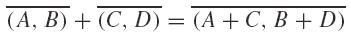
where A, B). We denote by is the equivalence class of ( the inverse of for the interval addition.

We have X = [-a, -a], and where - = . If X = [a, a], a ∈ ℝ, then . In this case, we identify X = [a, a] with a and we denote always by ℝ the subset of intervals of type [a, a]. = =

Naturally, the group ² by the isomorphism a - c, b - d). We find the notion of generalized interval and this yields immediately to the following result: → ( is isomorphic to the additive group ℝ

Proposition 1. Let 𝒳 = ∈ , and l: 𝕀ℝ ⟼ ℝ which gives the interval length. Thus

1. If l(Y) < l(X), there is an unique A ∈ 𝕀ℝ \ ℝ such that 𝒳 = ,

2. If l(Y) > l(X), there is an unique A ∈ 𝕀ℝ \ ℝ such that 𝒳 = , =

3. If l(Y) = l(X), there is an unique A = α ∈ ℝ such that 𝒳 = = .

Any element 𝒳 = A ∈ 𝕀ℝ - ℝ is said positive and we write 𝒳 > 0. Any element 𝒳 = A ∈ 𝕀ℝ - ℝ is said negative and we write 𝒳 < 0. We write 𝒳 ≥ 𝒳' if 𝒳 \ 𝒳' ≥ 0. For example if 𝒳 and 𝒳' are positive, 𝒳 ≥ 𝒳' ⇔ l(𝒳) ≥ l(𝒳'). The elements with α ∈ ℝ* are neither positive nor negative. with with

In ¹⁸, one defines on the abelian group , a structure of quasi linear space. Our approach is a little bit different. We propose to construct a real vector space structure. We consider the external multiplication:

defined, for all A ∈ 𝕀ℝ, by

for all α > 0. If α < 0 we put β = -α. So we put:

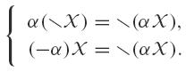
We denote α 𝒳 instead of α · 𝒳. This operation satisfies

• 1. For any α ∈ ℝ and 𝒳 ∈ we have:

• 2. For all α, β ∈ ℝ, and for all 𝒳, 𝒳' ∈ , we have

Theorem 1. The triplet (and 𝒳₂ = ofdetermine a basis of.. So dimℝ, +, .) is a real vector space and the vectors 𝒳1 = = 2

Proof. We have the following decompositions:

The linear map

defined by

is a linear isomorphism and ². is canonically isomorphic to ℝ

Definition 1. (is called the vector space of pseudo-intervals., +, )

2.2 A 4-dimensional free algebra associated with 𝕀ℝ

Consider the following subset of 𝒫1:

One observes that the semi-group 𝕀ℝ can be identified to 𝒫1,1 ∪ 𝒫1,2 ∪ 𝒫1,3. Let us consider as well the following vectors of ℝ2

They correspond to the intervals [1, 1],[0, 1],[-1, 0], and [-1, -1]. Any point of 𝒫1,1 ∪ 𝒫1,2 ∪ 𝒫1,3 admits the decomposition

(a, b) = α1e1 + α2e2 + α3e3 + α4e4

With αi ≥ 0. The dependance relations between the vectors ei are

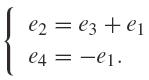
Thus there exists a unique decomposition of (a, b) in a chosen basis such that the coefficients are non negative. These basis are {e1, e2} for 𝒫1,1, {e2, e3} for 𝒫1,2, {e3, e4} for 𝒫1,3. Let us consider the free algebra of basis {e1, e2, e3, e4} whose products correspond to the Minkowski products. The multiplication table is

e1 e2 e3 e4 e1 e1 e2 e3 e4 e2 e2 e2 e3 e3 e3 e3 e3 e2 e2 e4 e4 e3 e2 e1

	e1	e2	e3	e4
e1	e1	e2	e3	e4
e2	e2	e2	e3	e3
e3	e3	e3	e2	e2
e4	e4	e3	e2	e1

Definition 2. This algebra is associative and its elements are called pseudo-intervals.

2.3 Pseudo-intervals product

Let φ: ₄ the natural injective embedding, F ⊂ 𝒜₄ the linear subspace generated by{e ₁ - e ₂ + e ₃, e ₁ + e ₄}, ψ the canonical embedding from 𝒜₄ to 𝒜₄/F and φ' = ψ ○ φ ^{1), (5), (13}. We identify an interval with its image in 𝒜₄. The application φ is not bijective. Its image on the elements 𝒳 = → 𝒜 = is

Theorem 2. The multiplication

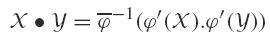
is distributive with respect the addition.

Proof. Practically the multiplication of two intervals will so be made: let X, Y ∈ ℝ. Thus X = Σα_ie_i , Y = Σβ_ie_i with α_i, β_i ≥ 0 and we have the product

this product is well defined because . This product is distributive because ∈

Remark. We have

We shall be careful not to return in 𝕀ℝ during the calculations as long as the result is not found. Otherwise we find the semantic problems of the distributivity.

We extend naturally the map φ: 𝕀ℝ → 𝒜4 to by

for every A ∈ 𝕀ℝ.

2.4 Pseudo-intervals division

Division between intervals can also be defined with solving X · Y = (1, 0, 0, 0) in 𝒜₄ or in a isomorphic algebra 𝒜₄'. In 𝒜₄ we consider the change of basis

This change of basis shows that 𝒜₄ is isomorphic to 𝒜₄'

e 1 e 2 e 3 e 4 e 1 e 1 0 0 e 4 e 2 0 e 2 e 3 0 e 3 0 e 3 e 2 0 e 4 e 4 0 0 e 1

	e 1	e 2	e 3	e 4
e 1	e 1	0	0	e 4
e 2	0	e 2	e 3	0
e 3	0	e 3	e 2	0
e 4	e 4	0	0	e 1

The unit of 𝒜₄' is the vector e ₁ + e ₂. This algebra is a direct sum of two ideals: 𝒜₄' = I ₁ + I ₂ where I ₁ is generated by e ₁ and e ₄ and I ₂ is generated by e ₂ and e ₃. It is not an integral domain, that is, we have divisors of 0. For example e ₁ · e ₂ = 0.

Proposition 2. The multiplicative group 𝒜₄* of invertible elements of 𝒜₄ is the set of elements x = (x ₁ , x ₂ , x ₃ , x ₄) such that

This means that the invertible intervals do not contain 0. If x ∈ 𝒜₄* we have:

2.5 Pseudo-intervals monotonicity property

Let us compute the product of pseudo-intervals using the product in 𝒜₄ and compare it with the Minkowski product. Let X = [a, b] and Y = [c, d] two intervals.

Lemma 1. If X and Y are not in the same piece 𝒫_{1, i}, then X ● Y corresponds to the Minkowski product.

Proof. i) If X ∈ 𝒫_1,1 and Y ∈ 𝒫_1,2 then φ(X) = (a, b - a, 0, 0) and φ(Y) = (0, d, -c, 0). Thus

ii) If X ∈ 𝒫_1,1 and Y ∈ 𝒫_1,3 then φ(X) = (a, b -a, 0, 0) and φ(Y) = (0, 0, d -c, -d). Thus

iii) If X ∈ 𝒫_1,2 and Y ∈ 𝒫_1,3 then φ(X) = (0, b, -a, 0) and φ(Y) = (0, 0, d -c, -d). Thus

Lemma 2. If X an Y are both in the same piece 𝒫_1,1 or 𝒫_1,3 , then the product X ● Y corresponds to the Minkowski product.

The proof is analogous to the previous.

Let us assume that X = [a, b] and Y = [c, d] belong to 𝒫_1,2. Thus φ(X) = (0, b, -a, 0) and φ(Y) = (0, d, -c, 0). We obtain

XY = (be ₂ - ae ₃)(de ₂ - ce ₃) = (bd + ac)e ₂ + (-bc - ad)e ₃.

Thus

[a, b][c, d] = [bc + ad, bd + ac].

This result is greater that all the possible results associated with the Minkowski product. However, we have the following property:

Proposition 3 Monotony property: Let 𝒳₁, 𝒳₂ ∈ . Then

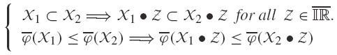
The order relation on 𝒜4 that ones uses here is

Proof. Let us note that the second property is equivalent to the first. It is its translation in . We can suppose that 𝒳1 and 𝒳2 are intervals belonging moreover to 𝒫1,2: φ(𝒳1) = (0, b, -a, 0), φ(𝒳2) = (0, d, -c, 0). Ifφ(𝒵) = (z1, z2, z3, z4), then

Thus

But (b - d), -(a - c) ≤ 0 and z2, z3 ≥ 0. This implies (𝒳1 ● 𝒵) ≤ (𝒳2 ● 𝒵).

2.6 The algebras 𝒜n and a better result of the product

We can refine the product to become closer to Minkowski's one. Consider the one dimensional extension 𝒜4 ⊕ ℝe5 = 𝒜5, where e5 is a vector corresponding to the interval [-1, 1] of 𝒫1,2. The multiplication table of 𝒜5 is

e1 e2 e3 e4 e5 e1 e1 e2 e3 e4 e5 e2 e2 e2 e3 e3 e5 e3 e3 e3 e2 e2 e5 e4 e4 e3 e2 e1 e5 e5 e5 e5 e5 e5 e5

	e1	e2	e3	e4	e5
e1	e1	e2	e3	e4	e5
e2	e2	e2	e3	e3	e5
e3	e3	e3	e2	e2	e5
e4	e4	e3	e2	e1	e5
e5	e5	e5	e5	e5	e5

The piece 𝒫1,2 is written 𝒫1,2 = 𝒫1,2,1 ∪ 𝒫1,2,1 where 𝒫1,2,1 = {[a, b], -a ≤ b} and 𝒫1,2,2 = {[a, b], -a ≥ b}. If X = [a, b] ∈ 𝒫1,2,1 and Y = [c, d] ∈ 𝒫1,2,2, thus

φ(X) . φ(Y) = (0, b + a, 0, 0, -a).(0, 0, -c -d, 0, d) = (0, -(a + b)(c + d), 0, 0, a(c + d) + bd).

Thus we have

X ● Y = [-bd -ac -ad, -bc].

Example. Let X = [-2, 3] and Y = [-4, 2]. We have X ∈ 𝒫1,2,1 and Y ∈ 𝒫1,2,2. The product in 𝒜4 gives

X ● Y = [-16, 14].

The product in 𝒜5 gives

X ● Y = [-12, 10].

The Minkowski product is

[-2, 3].[-4, 2] = [-12, 8].

Thus the product in 𝒜5 is better than the product in 𝒜4 with respect to the partial order. Let's go further. Considering a partition of 𝒫1,2, we can define an extension of 𝒜4 of dimension n, the choice of n depends on the approach wanted of the Minkowski product. For example, let us consider the vector e6 corresponding to the interval [-1, 1/2]. Thus the Minkowsky product gives e6 * e6 = e7 where e7 corresponds to[-1/2, 1]. This yields to the fact that 𝒜6 is not an associative algebra but it is the case for 𝒜7 whose table of multiplication is

e1 e2 e3 e4 e5 e6 e7 e1 e1 e2 e3 e4 e5 e6 e7 e2 e2 e2 e3 e3 e5 e6 e7 e3 e3 e3 e2 e2 e5 e7 e6 e4 e4 e3 e2 e1 e5 e7 e6 e5 e5 e5 e5 e5 e5 e5 e5 e6 e6 e6 e7 e7 e5 e7 e6 e7 e7 e7 e6 e6 e5 e6 e7

	e1	e2	e3	e4	e5	e6	e7
e1	e1	e2	e3	e4	e5	e6	e7
e2	e2	e2	e3	e3	e5	e6	e7
e3	e3	e3	e2	e2	e5	e7	e6
e4	e4	e3	e2	e1	e5	e7	e6
e5	e5	e5	e5	e5	e5	e5	e5
e6	e6	e6	e7	e7	e5	e7	e6
e7	e7	e7	e6	e6	e5	e6	e7

Example. Let X = [-2, 3] and Y = [-4, 2]. The decomposition on the basis {e1, ..., e7} with positive coefficients writes

X = e5 + 2e7, Y = 2e6.

X ● Y = (e5 + 2e7)(4e6) = 4e5 + 8e6 = [-12, 8].

We obtain now the Minkowski product.

Remark 1. Pseudo-intervals division can be defined as well in 𝒜5 and 𝒜7.

2.7 Inclusion functions

It is necessary for some problems to extend the definition of a function defined for real numbers f: ℝ → ℝ to function defined for intervals [f]: 𝕀ℝ → 𝕀ℝ such as [f]([a, a])=f(a) for any a ∈ ℝ. It will be convenient to have the same formal expression for f and [f]. Usually the lack of distributivity in Minkowski arithmetic does not give the possibility to get the same formal expressions. But with the pseudo-intervals arithmetic we have presented, there is no data dependency anymore and one can define easily inclusion functions from the natural one. For example, let's extend to intervals the real functions f0(x) = x2 - 2x + 1, f1(x) = (x - 1)2, f2(x) = x(x - 2) + 1. Usually, with the Minkwoski operations, the three expressions of this same function for the interval X = [3, 4] are [f]0(X) = [2, 11], [f]1(X) = [4, 9] and [f]2(X) = [6, 12]. Data dependancy occurs when the variable appears more than once in the function expression. The deep reason of that is the lack of distributivity in Minkowski arithmetic. But within the arithmetic developed in 𝒜4 or higher dimension free algebras [nicolas], this problem vanishes. For example: with X = [3, 4] and since X ∈ 𝒫11,

(2.2)

Since e ₁ = (1, 0, 0, 0), e ₂ = (0, 1, 0, 0) and with means of product table, one has

(2.3)

(2.4)

and

(2.5)

Thus, [f]₀(X) = [f]₁(X) = [f]₂(X) = [4, 9] and the inclusion function is defined univoquely regardless the way to write the original one.

On the other hand, the construction of the inclusion function depends on the type of problem one deals with. If one aims to perform set inversion for example, it has to be done in the semi-group 𝕀ℝ. But, the substraction is not defined in 𝕀ℝ. This problem can be circumvented by replacing it with an addition and a multiplication with the interval e ₄ = [-1, -1]. This maintains the associativity and distributivity of arithmetic and permits to introduce a pseudo-substraction. For example: if f(x) = x ² - x = x(x - 1) for real numbers, one defines [f](X) = X ² + e ₄ · X. One reminds the product [-1, -1]·[a, b] is equal to [-b, -a]. Due to the fact that the arithmetic is now associative and distributive, one does not have data dependency anymore and [f](X) = X ² + e ₄ · X = X · (X + e ₄). The last term corresponds to the transfer of x(x - 1). Division can be transferred to the semi-group in the same way by replacing 1/x = x ^-1 with X^{e 4}.

Taylor polynomial expansions, differential calculus and linear algebra operations are defined only in a vector space. Therefore the transfer for the vector space is done directly. This permits to get infinitesimal intervals with the substraction and to compute derivatives. This is of course not allowed and not possible into the semi-group. From 𝕀ℝ to the vector space X. This means that [a, b] substraction is the anti-interval [-a, -b] addition. One of the most important consequence is that it is possible to transfer some functions directly to the pseudo-intervals. For example, it is easy to prove analytically in with means of Taylor expansion., f: x ⟼ -x is transferred to [f]: X ≡ = ⟼ that [exp] ≡ \

2.8 Numerical linear algebra examples

One uses the 𝒜₇ pseudo-intervals arithmetic for simple examples of linear algebra computations where matrix elements are intervals.

2.8.1 Interval matrix diagonalization

As an example, we would like to compute the largest eigenmode of the matrix M whose elements are intervals centered around a certain real number with a radius є:

If one uses scilab to compute the spectrum of the previous matrix without radius (є = 0), the highest eigenvalue is approximatively 16.345903 and the corresponding eigenvector is (0.4728057, 0.5716783, 0.6705510). In order to show that arithmetics and interval algebra developed above are robust and stable, let's try to compute the highest eigenvalue of an interval matrix. One uses here the iterate power method, which is very simple and constitute the basis of several powerful methods such as deflation and others.

The Figures 1 and 2 show clearly for different value of є the stability of the multiplication, and the largest eigenmode is recovered when є = 0. The other eigen modes can be computed with the deflation methods for example which consists to withdraw the direction spanned by the eigenvector associated to the highest eigenvalue to the matrix by constructing its projector and to do the same. Several methods are available and efficient to achieve that ^{6), (35}. We have choosen to compute only the highest eigenvalue and its corresponding eigenvector in order to show simply the efficiency of our new arithmetic.

Figure 1:
Largest eigenvalue convergence computed with iterate power method to the value computed with scilab 16.345903.

Figure 2:
Eigenvector components associated to the largest eigenvalue convergence computed with iterate power method to the eigenvector computed with scilab (0.4728057, 0.5716783, 0.6705510).

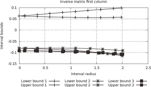
2.8.2 Interval matrix inversion

Let's define the matrix X whose elements are intervals centered around a certain real number with a radius є:

Scilab inversion function gives numerically for є = 0

(2.6)

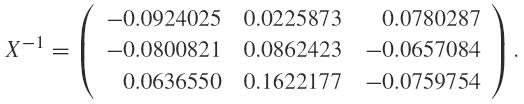
We would like to use the well-known Schutz-Hotelling algorithm ^{6), (35} to inverse the matrix X since it uses simple arithmetic operations:

(2.7)

The elements of inverse matrix columns are exhibited on Figures 3, 4, 5 and are converging to the right values when є = 0.

Figure 3:
First column elements bounds convergence according interval radius є.

Figure 4:
Second column elements bounds convergence according interval radius є.

Figure 5:
Third column elements bounds convergence according interval radius є.

3 TOPOLOGY OF 𝕀ℝ

One shows in this section that can be endowed with the metric topology of a Banach space. This permits to define correctly continuity and differentiability of functions.

3.1 Banach space structure of 𝕀ℝ

Any element 𝒳 ∈ or . We define its length l(𝒳) as the length of A and its center as c(A) or -c(A) in the second case. is written

Theorem 3. The map || || : → ℝ⁺ given by

||𝒳|| = l(𝒳) + |c(𝒳)|

for any 𝒳 ∈ is a norm.

Proof. We have to verify the following axioms:

1) If ||𝒳|| = 0, then l(𝒳) = |c(𝒳)| = 0 and 𝒳 = 0.

2) Let λ ∈ ℝ. We have

||λ𝒳|| = l(λ𝒳) + |c(λ𝒳)| = |λ| · l(𝒳) + |λ| · |c(𝒳)| = |λ| · ||𝒳||.

3) One considers that I refers to 𝒳 and J refers to 𝒳' thus 𝒳 = or = . We have to study the two different cases:

i) If 𝒳 + 𝒳' = , then or

ii) Let𝒳 + 𝒳' = K + J = I and = then . If

that is

So we have a norm on .

Theorem 4. The normed vector space is a Banach space.

Proof. In fact, all the norms on ℝ² are equivalent and ℝ² is a Banach space for any norm. The vector space is then isomorphic to ℝ2. Thus, it is complete.

Remarks.

1. To define the topology of the normed space ₀ = a, b) ∈ ℝ². We assume that χ₀ = A ₁, ..., A ₄ the points A ₁ = (a - ε, b - ε), A ₂ = (a + ε/2, b - ε/2), A ₃ = (a + ε, b + ε), A ₄ = (a - ε/2, b + ε/2). If 0 < a < b, then the ε-neighborhood of χ₀ = A ₁, A ₂, A ₃, A ₄. for ε a positive infinitesimal number. We can give a geometrical representation, considering χ and ε an infinitesimal real number. Let is represented by the parallelograms whose vertices are represented by the point (, it is sufficient to describe the ε-neighborhood of any point χ0 ∈

2. We can consider another equivalent norms on . For example

||𝒳|| = ||\𝒳|| = max{|x|, |y|}

where 𝒳 = , but the initial one has a better geometrical interpretation.

3.2 Continuity and differentiability in 𝕀ℝ

As ₀ = X ₀, ε) = {X ∈ is a Banach space, we can describe a notion of differential function on it. Consider 𝒳.. The norm ||.|| defines a topology on whose a basis of neighborhoods is given by the balls ℬ( in = , ||𝒳 \ 𝒳0|| < ε}. Let us characterize the elements of ℬ(X0, ε). 𝒳0 =

Proposition 4. Consider 𝒳0 = inand ε ~ 0, ε > 0. Then every element of ℬ(X ₀, ε) is of type 𝒳 = and satisfies =

l(X) ∈ B _ℝ(l(X ₀), ε₁) and c(X) ∈ B _ℝ(c(X ₀), ε₂)

with ε₁, ε₂ ≥ 0 and ε₁ + ε₂ ≤ ε, where B _ℝ(x, a) is the canonical open ball in ℝ of center x and radius a.

Proof. First case: Assume that 𝒳 = = . We have

If l(X) ≥ l(X0) we have

As l(X) - l(X0) ≥ 0 and |c(X) - c(X0)| ≥ 0, each one of this term if less than ε. If l(X) ≤ l(X0) we have

||𝒳 \ 𝒳0|| = l(X0) - l(X) + |c(X0) - c(X)|.

and we have the same result.

Second case: Consider 𝒳 = = . We have

and

||𝒳 \ 𝒳0|| = l(X0) + l(X) + |c(X0) + c(X)|.

In this case, we cannot have ||𝒳 \ 𝒳0|| < ε thus X ∉ ℬ(X0, ε).

Definition 3. A function f:→is continuous at 𝒳₀ if

∀ε > 0, ∃η such that ||𝒳 \ 𝒳₀|| < η implies ||f(𝒳) \ f(𝒳₀)|| < ε.

Consider (𝒳₁, 𝒳₂) the basis of given in Section 2. We have

If f is continuous at 𝒳₀ so

f(𝒳) \ f(𝒳₀) = (f ₁(𝒳) - f ₁(𝒳₀)) 𝒳₁ + (f ₂(𝒳) - f ₂(𝒳₀)) 𝒳₂.

To simplify notations let α = f ₁(𝒳) - f ₁(𝒳₀) and β = f ₂(𝒳) - f ₂(𝒳₀). If ||f(𝒳) \ f(𝒳₀)|| < ε, and if we assume f ₁(𝒳) - f ₁(𝒳₀) > 0 and f ₂(𝒳) - f ₂(𝒳₀) > 0 (other cases are similar), then we have

Thus f ₁(𝒳) - f ₁(𝒳₀) < ε. Similarly,

and this implies that f ₂(𝒳) - f ₂(𝒳₀) < ε.

Corollary 1. f is continuous at 𝒳₀ if and only if f ₁ and f ₂ are continuous at 𝒳₀ .

Definition 4. Consider 𝒳₀ inand f:→continuous. We say that f is differentiable at 𝒳₀ if there exists a linear function g:→such that

||f(𝒳) \ f(𝒳₀) \ g(𝒳 \ 𝒳₀)|| = o(||𝒳 \ 𝒳₀||).

Examples.

• f(𝒳) = 𝒳. This function is continuous and differentiable at any point. Its derivative is f'(𝒳) = 1.

• f(𝒳) = 𝒳². Consider 𝒳₀ = X ₀, ε). We have = and 𝒳 ∈ ℬ(

Given ε > 0, let η = , thus if ||𝒳 \ 𝒳0|| < η, we have ||𝒳2 \ 𝒳20|| < ε and f is continuous and differentiable. It is easy to prove that f'(𝒳) = 2𝒳 is its derivative.

• Consider P = a0 + a1X + ... + anXn ∈ ℝ[𝕏]. We define f: f(𝒳) = a ₀𝒳₂ + a ₁𝒳 + ... + a_n ⁿ 𝒳ⁿ where 𝒳ⁿ = 𝒳 - 𝒳^{n -1}. From the previous example, all monomials are continuous and differentiable, it implies that f is continuous and differentiable as well. → with

• Consider the function Q ₂ given by Q ₂([x, y]) = [x ², y ²] if |x| < |y| and Q ₂([x, y] = [y ², x ²] in the other case. This function is not differentiable.

3.3 Minimization examples

One uses the 𝒜₇ pseudo-intervals arithmetic for simple examples of inclusion function minimization with first and second order methods such as respectively fixed-step gradient descent and Newton-Raphson ones.

3.3.1 Fixed-step gradient descent method

Let's minimize the function x ⟼ x · exp(x) with fixed-step gradient method which belongs to the so-called gradient descent method ³⁵. This example is very simple but it shows that the result is garanted to be found within the final interval. One sets initial guess interval to [-5, 2], fixed-step of descent to10^-2, finite difference step to 10^-3 and accuracy of gradient to 10^-3. The results shown in Figures 6, 7) show that for any initial guess the interval width decreases to converge to real point minimum.

Figure 6:
Convergence of the fixed-step gradient algorithm for the function x ⟼ x · exp(x) to an interval centered around [-1, -1] = -1.

Figure 7:
Convergence of the fixed-step gradient algorithm for the derivative of the function x ⟼ x · exp(x) to an interval centered around [0, 0] = 0.

3.3.2 Newton-Raphson method

Let's optimize the same function x ⟼ x · exp(x) with a second order method such as the Newton-Raphson one, which is the basis of all second order methods such as Newton or quasi-Newton's ones ³⁵. One sets initial guess interval to [0, 10], finite difference step to 10^-3 and accuracy of gradient to10^-9. One can state on Figures (8, 9) that it finds the same minimum which is an interval centered around -1.

Figure 8:
Convergence of the Newton-Raphson algorithm for the function x ⟼ x · exp(x) to an interval centered around [-1, -1] = -1.

Figure 9:
Convergence of the Newton-Raphson algorithm for the derivative of the function x ⟼ x · exp(x) to an interval centered around [0, 0] = 0.

4 CONCLUSION

We have presented a better algebraic way to do calculations on intervals, called pseudo-intervals vector space or free algebra. This approach ^{1), (5), (13} is done by embedding the space of intervals into a free algebra of dimension belonging to {4, 5, 7}. It permits to obtain all the basic arithmetic operators with distributivity and associativity. We have shown that when one increases the representative algebra dimension, the multiplication result will be closer to the usual Minkowski product. It is now possible to build inclusion functions from the natural ones in a systematicway. Thus, it allows to build all algebraic operations and functions on intervals and avoids completely the wrapping effects and data dependance. One has exhibited some simple examples of applications: minimization, diagonalization and inversion of matrices which clearly state that the arithmetic is stable and that if the initial data are known with uncertainity (belonging to an interval), it is thus possible to estimate with accuracy the point solution of the problem, a real number or an interval centered around it. This pseudo-intervals arithmetic seems to be a promising and powerful computation framework in several domains of sciences and engineering, such as physics, mechanics of structure, or finance for instance.

5 ACKNOWLEDGEMENTS

The author thanks Michel Gondran for useful and interesting discussions.

REFERENCES

• ¹
  B. Durand, A. Kenoufi & J.F. Osselin. System adjustments for targeted performances combining symbolic regression and set inversion. Inverse problems for science and engineering, (2013).
• ²
  A. Trepat, E. Gardenes & H. Mielgo. Modal intervals: Reason and ground semantics. Lecture Notes in Computer Science, Springer-Verlag, Berlin, Heidelberg, 212 (1986), 27-35.
• ³
  L. Jorba, R. Calm, R. Estela, H. Mielgo, A. Trepat, E. Gardenes & M.A. Sainz. Modal intervals. Reliable Computing, 7 (2001), 77-111.
• ⁴
  E. Gardenes. Fundamentals of sigla, an interval computing system over the completed set of intervals. Computing, 24 (1980), 161-179.
• ⁵
  N. Goze. PhD thesis, N-ary algebras and interval arithmetics. University of Haute-Alsace, (2011).
• ⁶
  A.S. Householder. The theory of matrices in numerical analysis. Dover Publications, (1975).
• ⁷
  http://www.ti3.tu-harburg.de/rump/intlab/
  » http://www.ti3.tu-harburg.de/rump/intlab/
• ⁸
  E. Kaucher. Ueber metrische und algebraische Eigenschaften einiger beim numerischen Rechnen auftretender Raume. Dissertation, Universitaet Karlsruhe, (1973).
• ⁹
  E. Kaucher. Algebraische erweiterungen der intervallrechnung unter erhaltung der ordnungs und verbandstrukturen computing. 1 (1977), 65-79.
• ¹⁰
  E. Kaucher. Ueber eigenschaften und en der anwendungsmoeglichkeiten der erweiterten intervallrechnung und des hyperbolischen fastkoerpers ueber r computing. 1 (1977), 81-94.
• ¹¹
  E. Kaucher. Interval analysis in the extended interval space ir computing. 2 (1980), 33-49.
• ¹²
  R.B. Kearfott. Rigorous Global Search: Continuous Problems. Academic Publishers, (1996).
• ¹³
  A. Kenoufi. Probabilist set inversion using pseudo-intervals arithmetic. Trends in Applied and Computational Mathematics, 15 (1) (2014), 97-117.
• ¹⁴
  O. Didrit, L. Jaulin, M. Kieffer & E. Walter. Introduction to interval Analysis. SIAM 2009, Applied interval Analysis. Springer-Verlag, London, (2001).
• ¹⁵
  S.M. Markov. Extended interval arithmetic involving infinite intervals. Mathematica Balkanica, New Series, 6(3) (1992), 269-304.
• ¹⁶
  S.M. Markov. On directed interval arithmetic and its applications. J. UCS, 1(7) (1995), 510-521.
• ¹⁷
  S.M. Markov. On the Foundations of Interval Arithmetic. Scientific Computing and Validated Numerics Akademie Verlag, Berlin, (1996).
• ¹⁸
  M. Markov. Isomorphic embeddings of abstract interval systems. Reliable Computing, (3) (1997), 199-207.
• ¹⁹
  http://maxima.sourceforge.net
  » http://maxima.sourceforge.net
• ²⁰
  R.E. Moore. PhD thesis. Standford university, (1962).
• ²¹
  R.E. Moore. Interval analysis. Prentice Hall, Englewood Cliffs, NJ, (1966).
• ²²
  R.E. Moore. A test for existence of solutions to nonlinear systems. SIAM J. Numer. Anal., 14(4) (1977), 611-615.
• ²³
  E. Popova, N. Dimitrova & S. M. Markov. Extended Interval arithmetic: New Results and Applications. Computer Arithmetic and Enclosure Methods. Elsevier Sci. Publishers B.V., (1992).
• ²⁴
  H.J. Ortolf. Eine verallgemeinerung der intervallarithmetik. geselschaft fuer mathematik und datenverarbeitung. Bonn, 11 (1969), 1-71.
• ²⁵
  E.D. Popova. All about generalized interval distributive relations. i. complete proof of the relations. Sofia, (2000).
• ²⁶
  E.D. Popova. Multiplication distributivity of proper and improper intervals. Reliable Computing, 7(2) (2001), 129-140.
• ²⁷
  Yves Deville, Pascal Van Hentenryck & Laurent Michel. Numerica: A Modelling Language for Global Optimization. MIT Press, (1997).
• ²⁸
  http://www.python.org
  » http://www.python.org
• ²⁹
  C.T. Yang & R.E. Moore. Interval analysis i. LMSD-285875, Lockheed Aircraft Corporation, Missiles and Space Division, Sunnyvale, California, (1959).
• ³⁰
  Wayman Strother, R.E. Moore & C.T. Yang. Interval integrals. LMSD-703073, Lockheed Aircraft Corporation, Missiles and Space Division, Sunnyvale, California, IX(4) (1960), 241-245.
• ³¹
  http://www.sagemath.org
  » http://www.sagemath.org
• ³²
  T. Sunaga. Theory of an interval Algebra and its Application to Numerical Analysis. Number 2. RAAG Memoirs, (1958).
• ³³
  Mieczyslaw Warmus. Calculus of approximations. Bull. Acad. Pol. Sci., C1, III(IV (5)) (1956), 253-259.
• ³⁴
  Mieczyslaw Warmus. Approximations and inequalities in the calculus of approximations. classification of approximate numbers. Bull. Acad. Pol. Sci. math. astr. & phys., IX(4) (1961), 241-245.
• ³⁵
  W.T. Vetterling, B.P. Flannery, W.H. Press & S.A. Teukolsky. Numerical Recipes in C: The Art of Scientific Computing, 2nd Ed. Cambridge University Press, New York, (1992).

Publication Dates

• Publication in this collection
  Sep-Dec 2016

History

• Received
  13 Oct 2014
• Accepted
  30 Aug 2016