ABSTRACT:
This work presents the development of a three-dimensional (3D) model of an outcrop of the Corumbataí Formation (Permian, Paraná Basin, Brazil) using Structure from Motion - Multi-View Stereo (SfM-MVS) technique in order to provide a structural analysis of clastic dikes cutting through siltstone layers. While traditional photogrammetry requires the user to input a series of parameters related to the camera orientation and its characteristics (such as focal distance), in SfM-MVS the scene geometry, camera position and orientations are automatically determined by a bundle adjustment, an iterative procedure based on a set of overlapping images. It is considered a low-cost technique in terms of hardware and software, also being able to provide point density and accuracy on par to the ones obtained withTerrestrial Laser Scanning. The results acquired on this research have good agreement with previous works, yielding a NNW main orientation for the dikes measured in the field and on the 3D model. The development of this work showed that SfM-MVS use and practice on geosciences still needs more studies on the optimization of the involved parameters (such as camera orientation, image overlap and angle of illumination), which, when accomplished, will result in less processing time and more accurate models.
KEYWORDS:
clastic dikes; structure from motion; digital outcrop model; photogrammetry; structural geology
INTRODUCTION
In geology, the understanding of structures can be too complex to be reached using only field methods. Remote sensing topographic survey techniques such as LiDAR (Light Detection And Ranging, also called laser scanning), and photogrammetry are able to provide greater amount of information, as their resulting digital models allow (Bistacchi et al. 2015Bistacchi A., Balsamo F., Storti F., Mozafari M., Swennen R., Solum J., Tueckmantel C., Taberner C. 2015. Photogrammetric digital outcrop reconstruction, visualization with textured surfaces, and three-dimensional structural analysis and modeling: Innovative methodologies applied to fault-related dolomitization (Vajont Limestone, Southern Alps, Italy). Geosphere, 11(6):2031-2048. https://doi.org/10.1130/GES01005.1
https://doi.org/10.1130/GES01005.1...
, Hodgetts 2013Hodgetts D. 2013. Laser scanning and digital outcrop geology in the petroleum industry: A review. Marine and Petroleum Geology, 46:335-354. https://doi.org/10.1016/j.marpetgeo.2013.02.014
https://doi.org/10.1016/j.marpetgeo.2013...
):
-
Detailed quantitative description of geological features regarding geometry and spatial relationships;
-
Collection of large amounts of data, evenly distributed along an area or outcrop, providing a statistical basis for modeling;
-
Unified analysis of large-scale outcrops, even at reservoir scale;
-
True and reliable documentation that can be used for multiple purpose;
-
Three-dimensional (3D) outcrop navigation/exploration, providing “access”to out-of-reach or hazardous areas.
Among such techniques, SfM-MVS (Structure from Motion - Multi-View Stereo) workflow has gained strength in the geosciences over the past years (Tab. 1), mostly because when compared to other digital surveying it is capable of producing high-resolution data at low cost, fast and virtually independent of spatial scale. The final result of SfM-MVS is a detailed 3D model - also referred by some authors as Digital Outcrop Model (DOM) (Pringle et al. 1999Pringle J.K., Crawford D.C., Clark J.D., Gardiner A., Westerman A.R., Morgan B.E.F., Green S. 1999. A novel technique integrating digital photogrammetry with geological and geophysical data to acquire 3D architectures at Alport Castles, Derbyshire, UK. In: BSRG Annual Conference, Edinburgh. Annals…, Zahm et al. 2016Zahm C., Lambert J., Kerans C. 2016. Use of Unmanned Aerial Vehicles (UAVs) to create Digital Outcrop Models: an example from the Cretaceous Cow Creek Formation, Central Texas. Gulf Coast Association of Geological Societies Journal, 5:180-188. Available at: <Available at: http://archives.datapages.com/data/gcags-journal/data/005/005001/pdfs/180.htm
>. Accessed on: August, 2018.
http://archives.datapages.com/data/gcags...
, Silva et al. 2014Silva R., Veronez M., Tognoli F.M., Souza M., Inocêncio L. 2014. Accuracy Analysis of Digital Outcrop Models Obtained from Terrestrial Laser Scanner (TLS). International Journal of Advanced Remote Sensing and GIS, 3:508-515. Available at: <Available at: http://technical.cloud-journals.com/index.php/IJARSG/article/view/Tech-149
>. Accessed on: August, 2018.
http://technical.cloud-journals.com/inde...
), or virtual outcrop (Pringle et al. 2001Pringle J.K., Clark J.D., Westerman A.R., Stanbrook D.A., Gardiner A.R., Morgan B.E. 2001. Virtual outcrops: 3-D reservoir analogues. Journal of the Virtual Explorer, 4(9). https://doi.org/10.3809/jvirtex.2001.00036
https://doi.org/10.3809/jvirtex.2001.000...
, Tavani et al. 2014Tavani S., Granado P., Corradetti A., Girundo M., Iannace A., Arbués P., Munõz J., Mazzoli S. 2014. Building a virtual outcrop, extracting geological information from it, and sharing the results in Google Earth via OpenPlot and Photoscan: An example from the Khaviz Anticline (Iran). Computers and Geosciences, 63:44-53. https://doi.org/10.1016/j.cageo.2013.10.013
https://doi.org/10.1016/j.cageo.2013.10....
) -, that can be used as a point cloud or as a triangular mesh. As shown in Table 1, most applications of SfM-MVS are dedicated to extraction of geometrical properties of discontinuities, mostly faults and fractures, which are simple structures. An example of a complex structure that can take advantage of the use of SfM-MVS are clastic dikes, which are discordant subvertical sheets, tabular bodies of clastic sediments that can form by hydraulic fracturing and infilling (Hargitai & Levi 2014Hargitai H., Levi T. 2014. Clastic Dike. In: Hargitai H., Kereszturi A. (Eds.), Encyclopedia of Planetary Landforms. New York: Springer, p. 1-9. https://doi.org/10.1007/978-1-4614-9213-9_99-1
https://doi.org/10.1007/978-1-4614-9213-...
). Even for traditional field survey, the analysis of such structures can be challenging and, to date, no work has presented it through the use of 3D models. Thus, the objectives of this paper are twofold:
-
use SfM-MVS to generate a DOM of an outcrop of the Corumbataí Formation (Permian, Paraná Basin), which contains a remarkable exposition of clastic dikes;
-
extract geological attitudes of clastic dikes from the DOM and compare them with field-collected data in order to discuss the pros and cons of using digitally-derived data in structural analysis.
Considering that the use of SfM-MVS in the geosciences is expanding rapidly, and that a successful DOM generation might involve more factors than initially considered by the non-experienced user, we also present a brief summary of the processes and algorithms involved in the SfM-MVS workflow, as well a list of best practices for fieldwork, derived from the experience gained by the authors in the development of this project.
STUDY AREA AND GEOLOGICAL SETTING
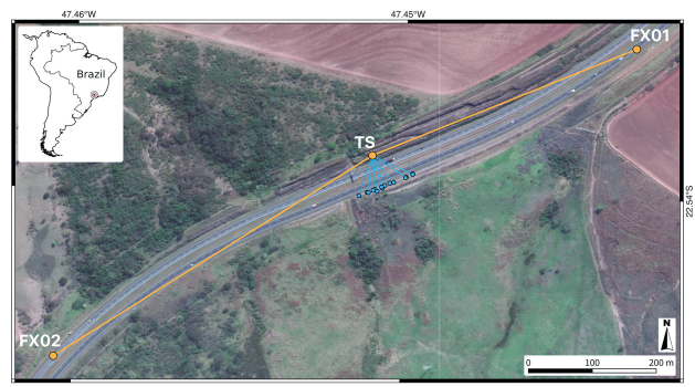
This study focused on a NE-SW (facing NW) roadside rocky outcrop near Limeira city, state of São Paulo, Brazil, km 161.5 of SP-348 Bandeirantes highway (Fig. 1). The outcrop is a ∼500 m-long and ∼30 m-high exposition of the Corumbataí Formation (Permian, Paraná Basin), composed of siltstone intercalated with fine sandstone and carbonate layers, intruded by a swarm of clastic dikes (Riccomini et al. 1992Riccomini C., Chamani M.A.C., Agena S.S., Fambrini G.L., Fairchild T.R., Coimbra A.M. 1992. Earthquake-induced liquefaction features in the Corumbataí Formation (Permian, Paraná Basin, Brazil) and the dynamics of Gondwana. Anais da Academia Brasileira de Ciências, 64:210., Perinotto et al. 2008Perinotto J.A.J., Etchebehere M.L.C., Simões L.S.A., Zanardo A. 2008. Diques clásticos na formação Corumbataí (P) no nordeste da Bacia do Paraná, SP: Análise sistemática e significações estratigráficas, sedimentológicas e tectônicas. Geociências, 27(4):469-491. Available at: <Available at: http://www.periodicos.rc.biblioteca.unesp.br/index.php/geociencias/article/view/3417
>. Accessed on: August, 2018.
http://www.periodicos.rc.biblioteca.unes...
, Turra 2009Turra B.B. 2009. Diques clásticos da Formação Corumbataí, Bacia do Paraná, no contexto da tectônica permotriássica do Gondwana Ocidental. MS Dissertation. Instituto de Geociências, Universidade de São Paulo, São Paulo. https://doi.org/10.11606/D.44.2009.tde-06072009-111626
https://doi.org/10.11606/D.44.2009.tde-0...
).

Study area location in Brazil (inset). Positioning of the total station (TS), fixed points (FX01 and FX02) and targets distributed on the outcrop surface (blue points).
Syn-depositional and postdepositional dikes are distinguished depending on time of fracture infilling (Allen 1982Allen J.R.L. 1982. Sedimentary Structures Their Character and Physical Basis. v. II. Volume 30B of Developments in Sedimentology. Amsterdam, New York: Elsevier.), and two subtypes can be categorized based on the formative process: injection clastic dikes and sedimentary (or depositional) dikes. The first type are liquefaction structures that form as water-saturated granular material experiences an increase in pore fluid pressure, typically occurring in cohesionless or nearly-cohesionless sediments and may be caused by cycles of sheer stresses during strong earthquake events (M > 6.5 - Hargitai & Levi 2014Hargitai H., Levi T. 2014. Clastic Dike. In: Hargitai H., Kereszturi A. (Eds.), Encyclopedia of Planetary Landforms. New York: Springer, p. 1-9. https://doi.org/10.1007/978-1-4614-9213-9_99-1
https://doi.org/10.1007/978-1-4614-9213-...
).
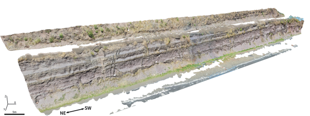
In the studied outcrop, clastic dikes are vertical to near-vertical tabular to ptygmatic-folded bodies of massive fine sandstone cutting through pelitic layers (Fig. 2). The dikes occur in four sedimentary levels, being more numerous on the lower level. The top of this level is marked by a well-defined surface with structures interpreted as sand extrusions. Despite the scattering of data, Turra (2009Turra B.B. 2009. Diques clásticos da Formação Corumbataí, Bacia do Paraná, no contexto da tectônica permotriássica do Gondwana Ocidental. MS Dissertation. Instituto de Geociências, Universidade de São Paulo, São Paulo. https://doi.org/10.11606/D.44.2009.tde-06072009-111626
https://doi.org/10.11606/D.44.2009.tde-0...
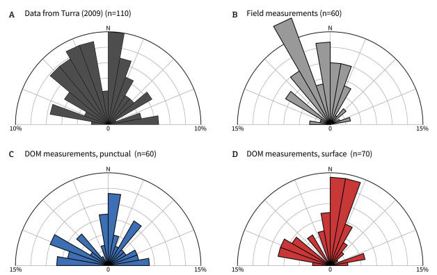
) described a general NNW orientation trend of clastic dikes and a N-NE trend of sand extrusions’ feeder dikes (Fig. 3A).

Perspective view of generated Digital Outcrop Model (DOM). See Supplemental Material for camera positions and ground control points (GCPs) (Suppl. Fig. S5 Supplementary data associated with this article can be found in the online version: Supplementary Table: S1 and Supplementary figures S1-S8. ).

Rose diagrams: (A) measurements from Turra (2009Turra B.B. 2009. Diques clásticos da Formação Corumbataí, Bacia do Paraná, no contexto da tectônica permotriássica do Gondwana Ocidental. MS Dissertation. Instituto de Geociências, Universidade de São Paulo, São Paulo. https://doi.org/10.11606/D.44.2009.tde-06072009-111626
https://doi.org/10.11606/D.44.2009.tde-0... ); (B) all field measurements; (C) Digital Outcrop Model (DOM) measurements (punctual); (D) DOM measurements (surface). All diagrams have 10º petals.
Riccomini et al. (1992Riccomini C., Chamani M.A.C., Agena S.S., Fambrini G.L., Fairchild T.R., Coimbra A.M. 1992. Earthquake-induced liquefaction features in the Corumbataí Formation (Permian, Paraná Basin, Brazil) and the dynamics of Gondwana. Anais da Academia Brasileira de Ciências, 64:210.) were the first authors to associate the formation of clastic dikes in the Corumbataí Formation to a seismic event. Later, Riccomini (1995Riccomini C. 1995. Tectonismo gerador e deformador dos depósitos sedimentares pós-gondvânicos da porção centro-oriental do Estado de São Paulo e áreas vizinhas. PhD Thesis. Instituto de Geociências, Universidade de São Paulo, São Paulo. https://doi.org/10.11606/T.44.2013.tde-03062013-103524
https://doi.org/10.11606/T.44.2013.tde-0...
) identified two sets of dikes orthogonal to each other with predominance in the NE-SW direction, interpreted as the direction of the maximum horizontal tension vector and associated with the early stages of the Pangea rupture. Chamani et al. (1992Chamani M.A., Martin M., Riccomini C. 1992. Estruturas de liqüefação induzidas por abalos sísmicos no permo-triássico da Bacia do Paraná, Estado de São Paulo, Brasil. In: Congresso Brasileiro de Geologia. Annals... p. 508-510.), Fernandes & Coimbra (1993Fernandes L., Coimbra A. 1993. Registros de episódios sísmicos na parte superior da Formação Rio do Rasto no Paraná, Brasil. In: Simpósio de Geologia do Sudeste. Annals…, p. 271-275.) and Riccomini et al. (1996Riccomini C., Sallun Filho W., Ferreira N., Coimbra A. 1996. Estruturas de liquefação em arenitos eólicos da Formação Botucatu (Ki) na Serra de Itaqueri, SP. In: Congresso Brasileiro de Geologia. Annals... p. 151-153.) also interpreted some features in the Permotriassic units of the Paraná Basin as seismites.
Perinotto et al. (2008Perinotto J.A.J., Etchebehere M.L.C., Simões L.S.A., Zanardo A. 2008. Diques clásticos na formação Corumbataí (P) no nordeste da Bacia do Paraná, SP: Análise sistemática e significações estratigráficas, sedimentológicas e tectônicas. Geociências, 27(4):469-491. Available at: <Available at: http://www.periodicos.rc.biblioteca.unesp.br/index.php/geociencias/article/view/3417
>. Accessed on: August, 2018.
http://www.periodicos.rc.biblioteca.unes...
), analyzing three different sites, concluded that due to the scatter of measurements the dikes occupied pre-existing fractures or those generated by hydrofracturing under local stress, being unrelated to regional tectonic patterns as suggested previously, although to Chamani (2015Chamani M.A. 2015. Tectônica Sinsedimentar no Siluro-Devoniano da Bacia do Parnaíba, Brasil: O Papel de Grandes Estruturas do Embasamento na Origem e Evolução de Bacias Intracratônicas. PhD Thesis, Instituto de Geociências, Universidade de São Paulo, São Paulo. https://doi.org/10.11606/T.44.2016.tde-04052016-111511
https://doi.org/10.11606/T.44.2016.tde-0...
) the lack of a careful statistical analysis (presenting orientation data only as great circles in a stereonet, for example) by Perinotto et al. (2008Perinotto J.A.J., Etchebehere M.L.C., Simões L.S.A., Zanardo A. 2008. Diques clásticos na formação Corumbataí (P) no nordeste da Bacia do Paraná, SP: Análise sistemática e significações estratigráficas, sedimentológicas e tectônicas. Geociências, 27(4):469-491. Available at: <Available at: http://www.periodicos.rc.biblioteca.unesp.br/index.php/geociencias/article/view/3417
>. Accessed on: August, 2018.
http://www.periodicos.rc.biblioteca.unes...
) hinders an objective assessment of their conclusions. The discussion brought by these works point to the uncertainty in interpreting clastic dikes and their associated structural markers, which justifies the experimentation of structural analysis based on SfM-MVS models as a more objective mean for assessing/ascertaining orientation data. Recent studies (Tohver et al. 2013Tohver E., Cawood P.A., Riccomini C., Lana C., Trindade R.I.F. 2013. Shaking a methane fizz: Seismicity from the Araguainha impact event and the Permian-Triassic global carbon isotope record. Palaeogeography, Palaeoclimatology, Palaeoecology, 387:66-75. http://dx.doi.org/10.1016/j.palaeo.2013.07.010
http://dx.doi.org/10.1016/j.palaeo.2013....
, 2018Tohver E., Schmieder M., Lana C., Mendes P.S.T., Jourdan F., Warren L., Riccomini C. 2018. End-Permian impactogenic earthquake and tsunami deposits in the intracratonic Paraná Basin of Brazil. GSA Bulletin, 130(7-8):1099-1120. https://doi.org/10.1130/B31626.1
https://doi.org/10.1130/B31626.1...
) related the seismicity that generated the dikes to the impact event that formed the Araguainha structure, at the Permian-Triassic boundary.
STRUCTURE FROM MOTION MULTI-VIEW STEREO
In the geosciences, the development of remote digital surveying methods allowed not only the increase in collection speed and data density, but also enabled the surveying in physically inaccessible places. Among such techniques, there are traditional photogrammetry, laser scanning and SfM-MVS.
Structure from Motion (SfM) is a recent tool that has had an impact on the field of geosciences in recent years. It enables the generation of high-precision 3D models from two-dimensional (2D) images in a simple way, bringing the power of digital models to non-experts. An important advantage of this method, compared with the traditional photogrammetric workflow, is that each feature is defined from a redundant number of photos (Snavely et al. 2006Snavely N., Seitz S.M., Szeliski R. 2006. Photo tourism: exploring photo collections in 3D. ACM Transactions on Graphics, 25(3):835-846. https://doi.org/10.1145/1179352.1141964
https://doi.org/10.1145/1179352.1141964...
), and error estimates are just another output from model inversion. This ensures the high quality of the results, because points with precision lower than a given threshold are automatically rejected by the inversion algorithm (Bistacchi et al. 2015Bistacchi A., Balsamo F., Storti F., Mozafari M., Swennen R., Solum J., Tueckmantel C., Taberner C. 2015. Photogrammetric digital outcrop reconstruction, visualization with textured surfaces, and three-dimensional structural analysis and modeling: Innovative methodologies applied to fault-related dolomitization (Vajont Limestone, Southern Alps, Italy). Geosphere, 11(6):2031-2048. https://doi.org/10.1130/GES01005.1
https://doi.org/10.1130/GES01005.1...
).
As put by Carrivick et al. (2016Carrivick J.L., Smith M.W., Quincey D.J. 2016. Structure from Motion in the Geosciences. West Sussex: John Wiley & Sons. https://doi.org/10.1002/9781118895818
https://doi.org/10.1002/9781118895818...
), most authors in geosciences cite in a simplified way the SfM algorithm as the sole responsible for creating the 3D model. When we look at the processing of the set of images, in brief, it goes through three main steps:
-
the recognition of points in common between the images of the set and the calculation of the x, y, z position of each point;
-
construction of a sparse point cloud (also referred as coarse cloud);
-
the refinement of the model and generation of a dense point cloud.
SfM algorithms are responsible only for the first two steps of the process. The third step is performed by the Multi-View Stereo (MVS) methods and, therefore, the most correct would be to refer to the SfM-MVS method.
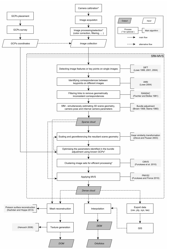
In this section, we would like to give a brief summary of the processes and algorithms involved in SfM-MVS workflow to generate a Digital Outcrop Model (DOM) (Fig. 4). Most of the information provided here is from the work of Carrivick et al. (2016Carrivick J.L., Smith M.W., Quincey D.J. 2016. Structure from Motion in the Geosciences. West Sussex: John Wiley & Sons. https://doi.org/10.1002/9781118895818
https://doi.org/10.1002/9781118895818...
) and the reader is referred to it for further detailing.

Simplified flowchart showing the main steps involved on a Digital Outcrop Model (DOM) generation using Structure from Motion - Multi-View Stereo workflow.
Image acquisition and ground control
As the name suggest, SfM-MVS is entirely dependent on images “in motion”, i.e., images taken from different viewpoints. Planning the image survey should consider several recommendations to ensure a high-quality 3D model.
There is a wide range of platforms that can be employed for the photo shooting and each of which has advantages and disadvantages that must be evaluated according to the application (Conlin et al. 2018Conlin M., Cohn N., Ruggiero P. 2018. A Quantitative Comparison of Low-Cost Structure from Motion (SfM) Data Collection Plat- forms on Beaches and Dunes. Journal of Coastal Research. https://doi.org/10.2112/JCOASTRES-D-17-00160.1
https://doi.org/10.2112/JCOASTRES-D-17-0...
). There are ground-based options including hand-held, the use of poles, tripods or rovers and airborne approaches using unmanned aerial vehicles (UAVs), kites, balloons and manned light aircrafts.
The images should provide a full coverage of the object or scene of interest, keeping a minimum 60% lateral and 30% vertical overlap, but these values may vary depending on the scene conditions. Camera positions should be well distributed around the object, avoiding “fan” methods (i.e., multiple images from a single point). Objects that produce low contrast require a higher percentage of overlap in order for the matches to be located and generate satisfactory results. For a feature to be digitally reconstructed, it must be observable in at least three images, so the number of images required for the reconstruction of an object or scene will then be a function of its size and the amount of overlap used.
Lighting conditions directly affect the quality of the DOM. Glare from reflective surfaces, variable contrast across a scene, the presence of shadows and changes in their length and surface albedo negatively affect point matching (Bemis et al. 2014Bemis S.P., Micklethwaite S., Turner D., James M.R., Akciz S., Thiele S.T., Bangash H.A. 2014. Ground-based and UAV-Based photogrammetry: A multi-scale, high-resolution mapping tool for structural geology and paleoseismology. Journal of Structural Geology, 69(Part A):163-178. https://doi.org/10.1016/j.jsg.2014.10.007
https://doi.org/10.1016/j.jsg.2014.10.00...
). Ideally the survey should occur under the same light conditions. Bright cloudy days - the exterior lighting equivalent of a dome light - are recommended, since the lighting is more uniform and the casting of shadows is reduced. In some cases, the use of artificial lights may be feasible and the arrangement must be composed of main light sources of the same intensity with diffusers to ensure no visible signs of the lighting sources in the object or scene.
The occurrence of gaps, holes or distortions in the DOM usually results from the inadequate application of such parameters. Ideally, the larger the set of images generated, the greater the overlap between images and, consequently, the higher the quality of the model. However, an excessive number of images are computationally expensive, generating very large models, which makes it difficult to manipulate and post-process. Pre-processing image data is an optional step to improve overall quality and can be performed using image filters to correct color, brightness and sharpness or selecting the most adequate images from the set.
When given no reference information, the SfM-MVS generates a point cloud within a relative reference system (Westoby et al. 2012Westoby M., Brasington J., Glasser N., Hambrey M., Reynolds J. 2012. ‘Structure-from-Motion’ photogrammetry: A low-cost, effective tool for geoscience applications. Geomorphology, 179:300-314. https://doi.org/10.1016/j.geomorph.2012.08.021
https://doi.org/10.1016/j.geomorph.2012....
), but, for the majority of applications in geosciences, information like distance, size, volume and orientation are essential and in order to get those it is necessary to acquire ground control. When only the scale is desired, it is necessary that the distance between two points is known, which can be obtained by field measuring the distance between two markers or by adding an object of known size in the scene, such as a ruler (Verma & Bourke 2018Verma A.K., Bourke M.C. 2018. A Structure from Motion photogrammetry-based method to generate sub-millimetre resolution Digital Elevation Models for investigating rock breakdown features. Earth Surface Dynamics Discussions, 1-34. https://doi.org/10.5194/esurf-2018-53
https://doi.org/10.5194/esurf-2018-53...
).
For greater accuracy and full 3D referencing or georeferencing, at least three ground control points (GCPs) are required. The points should be widely distributed on the scene, avoiding linear configuration. There is a wide range of options to mark out GCP locations such as printed targets (Riquelme et al. 2017Riquelme A., Cano M., Tomás R., Abellán A. 2017. Identification of Rock Slope Discontinuity Sets from Laser Scanner and Photogrammetric Point Clouds: A Comparative Analysis. Procedia Engineering, 191:838-845. https://doi.org/10.1016/j.proeng.2017.05.251
https://doi.org/10.1016/j.proeng.2017.05...
), spray paint (Viana et al. 2016Viana C.D., Endlein A., da Cruz Campanha G.A., Grohmann C.H. 2016. Algorithms for extraction of structural attitudes from 3D outcrop models. Computers and Geosciences, 90(Part A):112-122. https://doi.org/10.1016/j.cageo.2016.02.017
https://doi.org/10.1016/j.cageo.2016.02....
), spray-painted CD (Matthews 2008Matthews N.A. 2008. Aerial and Close-Range Photogrammetric Technology: Providing Resource Documentation, Interpretation, and Preservation. Technical Note 428. Technical Report. Denver, Colorado: U.S. Department of the Interior, Bureau of Land Management, National Operations Center. Available at: <Available at: https://www.blm.gov/download/file/fid/20806
>. Accessed on: August, 2018.
https://www.blm.gov/download/file/fid/20...
) or targets (Turner et al. 2012Turner D., Lucieer A., Watson C. 2012. An automated technique for generating georectified mosaics from ultra-high resolution Unmanned Aerial Vehicle (UAV) imagery, based on Structure from Motion (SFM) point clouds. Remote Sensing, 4(5):1392-1410. https://doi.org/10.3390/rs4051392
https://doi.org/10.3390/rs4051392...
), nails and colored flags (Haneberg 2008Haneberg W.C. 2008. Using close range terrestrial digital photogrammetry for 3-D rock slope modeling and discontinuity mapping in the United States. Bulletin of Engineering Geology and the Environment, 67(4):457-469. https://doi.org/10.1007/s10064-008-0157-y
https://doi.org/10.1007/s10064-008-0157-...
) or modeling clay (Jordá-Bordehore et al. 2017Jordá-Bordehore L., Riquelme A., Cano M., Tomás R. 2017. Comparing manual and remote sensing field discontinuity collection used in kinematic stability assessment of failed rock slopes. International Journal of Rock Mechanics and Mining Sciences, 97:24-32. https://doi.org/10.1016/j.ijrmms.2017.06.004
https://doi.org/10.1016/j.ijrmms.2017.06...
). The choice of the type of target must be made according to the conditions of the survey, considering that the size and the distinctiveness of the target in relation to its surroundings influence in the quality of the georeferencing. The GCPs survey is commonly done using Total Station or differential GPS, but for geological purposes great accuracy can be achieved using multiple approaches as shown by Sturzenegger and Stead (2009Sturzenegger M., Stead D. 2009. Close-range terrestrial digital photogrammetry and terrestrial laser scanning for discontinuity characterization on rock cuts. Engineering Geology, 106(3-4):163-182. https://doi.org/10.1016/j.enggeo.2009.03.004
https://doi.org/10.1016/j.enggeo.2009.03...
).
SfM-MVS workflow
There is a wide variety of SfM-MVS software, ranging from specific algorithms to stand-alone tools and web services. The commercial options include Pix4DMapper (Pix4D SA, 2017Pix4D SA. 2017. Pix4dmapper 3.2 user manual. Pix4D SA. Available at: <Available at: https://s3.amazonaws.com/mics.pix4d.com/manual_pdf/Pix4Ddesktop_Manual_3.2_May_2017.pdf
>. Accessed on: August, 2018.
https://s3.amazonaws.com/mics.pix4d.com/...
), PhotoModeler (Eos Systems Inc., 2014Eos Systems Inc. 2014. Photomodeler quick start guide. Eos Systems Inc. Available at: <Available at: https://www.photomodeler.com/order/PhotoModeler_QuickStartGuide.pdf
>. Accessed on: August, 2018.
https://www.photomodeler.com/order/Photo...
) and Agisoft PhotoScan (Agisoft, 2018Agisoft. 2018. Agisoft photoscan user manual professional edition, version 1.4. Agisoft. Available at: <Available at: http://www.agisoft.com/pdf/photoscan-pro_1_4_en.pdf
>. Accessed on: August, 2018.
http://www.agisoft.com/pdf/photoscan-pro...
). The latter is the most widely used in geosciences applications and the one used in this paper. Although commercial options are more user-friendly for non-experts, the main disadvantage is that their workflow is a black box, turning the identification of random and systematic errors difficult to handle (Ouédraogo et al. 2014Ouédraogo M.M., Degré A., Debouche C., Lisein J. 2014. The evaluation of unmanned aerial system-based photogrammetry and terrestrial laser scanning to generate DEMs of agricultural watersheds. Geomorphology, 214:339-355. https://doi.org/10.1016/j.geomorph.2014.02.016
https://doi.org/10.1016/j.geomorph.2014....
). To get around this problem some of the open source options include Bundler (Snavely et al. 2006Snavely N., Seitz S.M., Szeliski R. 2006. Photo tourism: exploring photo collections in 3D. ACM Transactions on Graphics, 25(3):835-846. https://doi.org/10.1145/1179352.1141964
https://doi.org/10.1145/1179352.1141964...
), PMVS (Furukawa & Ponce 2010Furukawa Y., Ponce J. 2010. Accurate, Dense, and Robust Multi-View Stereopsis. IEEE Transactions on Pattern Analysis and Machine Intelligence, 32(8):1362-1376. https://doi.org/10.1109/TPAMI.2009.161
https://doi.org/10.1109/TPAMI.2009.161...
), VisualSFM (Wu 2013Wu C. 2013. Towards linear-time incremental structure from motion. In: 3D Vision-3DV 2013, 2013 International Conference on, IEEE. Annals… p. 127-134. https://doi.org/10.1109/3DV.2013.25
https://doi.org/10.1109/3DV.2013.25...
, Wu et al. 2011Wu C., Agarwal S., Curless B., Seitz S.M. 2011. Multicore bundle adjustment. In: Computer Vision and Pattern Recognition (CVPR), 2011 IEEE Conference. Annals… p. 3057-3064. https://doi.org/10.1109/CVPR.2011.5995552
https://doi.org/10.1109/CVPR.2011.599555...
), OpenDroneMap (OpenDroneMap 2014OpenDroneMap. 2014. OpenDroneMap. Available at: <Available at: https://www.opendronemap.org/
>. Accessed on: August, 2018.
https://www.opendronemap.org/...
), Colmap (Schönberger et al. 2016Schönberger J.L., Zheng E., Frahm J.M., Pollefeys M. 2016. Pixelwise View Selection for Unstructured Multi-View Stereo. In: European Conference on Computer Vision (ECCV). Annals… p. 501-518. https://doi.org/10.1007/978-3-319-46487-9_31
https://doi.org/10.1007/978-3-319-46487-...
, Schönberger & Frahm 2016Schönberger J.L., Frahm J.M. 2016. Structure-from-Motion Revisited. In: Conference on Computer Vision and Pattern Recognition (CVPR). Annals… https://doi.org/10.1109/CVPR.2016.445
https://doi.org/10.1109/CVPR.2016.445...
) and MicMac (Rupnik et al. 2017Rupnik E., Daakir M., Deseilligny M.P. 2017. MicMac - a free, open-source solution for photogrammetry. Open Geospatial Data, Software and Standards, 2:14. https://doi.org/10.1186/s40965-017-0027-2
https://doi.org/10.1186/s40965-017-0027-...
).
Regardless of the software, as shown in Figure 4, the generic SfM-MVS process has around eight steps that may or may not constitute a single workflow. Ahead, we briefly describe each of the steps and algorithms commonly used in each one of them. It should be emphasized that the explanation provided here is simplified to be suitable for end users, since SfM-MVS is a combination of computer vision and traditional photogrammetry knowledge that goes beyond the scope of this work.
Given an image set, the first step is the detection of keypoints (common points between images) or feature points (sets of pixels) on single images. These points allow the different photos to be matched and the scene geometry to be reconstructed, but since the images are taken from multiple viewpoints it is a challenge to track those points. To solve this step, the scale-invariant feature transform (SIFT) object-recognition system (Lowe 1999Lowe D. 1999. Object recognition from local scale-invariant features. Proceedings of the Seventh IEEE International Conference on Computer Vision, 2:1150-1157. https://doi.org/10.1109/ICCV.1999.790410
https://doi.org/10.1109/ICCV.1999.790410...
, 2001Lowe D. 2001. Local feature view clustering for 3D object recognition. Proceedings of the 2001 IEEE Computer Society Conference on Computer Vision and Pattern Recognition. CVPR 2001. https://doi.org/10.1109/CVPR.2001.990541
https://doi.org/10.1109/CVPR.2001.990541...
, 2004Lowe D.G. 2004. Distinctive Image Features from Scale-Invariant Keypoints. International Journal of Computer Vision, 60(2):91-110. https://doi.org/10.1023/B:VISI.0000029664.99615.94
https://doi.org/10.1023/B:VISI.000002966...
) is the most popular approach. The performance of different region detectors is given in Mikolajczyk et al. (2005Mikolajczyk K., Tuytelaars T., Schmid C., Zisserman A., Matas J., Schaffalitzky F., Kadir T., Van Gool L. 2005. A comparison of affine region detectors. International Journal of Computer Vision, 65(1-2): 43-72. https://doi.org/10.1007/s11263-005-3848-x
https://doi.org/10.1007/s11263-005-3848-...
), and a comparison between other view-invariant local image descriptors is presented in Mikolajczyk & Schmid (2005Mikolajczyk K., Schmid C. 2005. A performance evaluation of local descriptors. IEEE Transactions on Pattern Analysis and Machine Intelligence, 27(10):1615-1630. https://doi.org/10.1109/TPAMI.2005.188
https://doi.org/10.1109/TPAMI.2005.188...
).
Once keypoints are located in each image, the second step consists of finding the correspondences between the keypoints on different images. The keypoint matching is performed by identifying the nearest neighbor for each keypoint in a database containing all the keypoints identified during the first step, but there is no guarantee that any given keypoint will have a partner at another image, so the discarding of points with no good matching is required. Since the SIFT keypoint descriptor has a 128-dimensional feature vector, some search implementations can be both difficult and computationally expensive. Lowe (2004Lowe D.G. 2004. Distinctive Image Features from Scale-Invariant Keypoints. International Journal of Computer Vision, 60(2):91-110. https://doi.org/10.1023/B:VISI.0000029664.99615.94
https://doi.org/10.1023/B:VISI.000002966...
) modifies the best-bin-first algorithm (Beis & Lowe 1997Beis J.S., Lowe D.G. 1997. Shape indexing using approximate nearest-neighbour search in high-dimensional spaces. In: Conference on Computer Vision and Pattern Recognition. Proceedings… IEEE Computer Society. p. 1000. Available at: <Available at: http://dl.acm.org/citation.cfm?id=794189.794431
>. Accessed on: August, 2018.
http://dl.acm.org/citation.cfm?id=794189...
) to cut off search after checking the first 200 nearest-neighbor candidates and only consider matches in which the nearest neighbor is less than 0.8 times the Euclidean distance to the second nearest-neighbor. This approach significantly increases the search speed with minimal loss in the number of correct matches and is known as approximate nearest neighbor (ANN).
Once the links between images have been established, the third step is responsible for filtering out geometrically inconsistent matches. The random sample consensus (RANSAC) method (Fischler & Bolles 1981Fischler M.A., Bolles R.C. 1981. Random sample consensus: a paradigm for model fitting with applications to image analysis and automated cartography. Communications of the ACM, 24(6):381-395. https://doi.org/10.1145/358669.358692
https://doi.org/10.1145/358669.358692...
) is the most commonly used to calculate the candidate fundamental matrices (a 3x3 matrix that “encode” the projective geometry between two views) over several iterations to filter out outliers and return the matrix with the largest number of inliers.
Using the geometrically consistent correspondences from the previous step, the fourth stage is the SfM itself, which consists of reconstructing simultaneously camera poses (position and orientation), 3D scene geometry and intrinsic camera calibration parameters. This is solved using a bundle adjustment (BA) (Brown 1958Brown D.C. 1958. A solution to the general problem of multiple station analytical stereotriangulation. Technical Report 43. RCA-MTP. Available at: <Available at: https://books.google.com.br/books?id=FikPPwAACAAJ
>. Accessed on: August, 2018.
https://books.google.com.br/books?id=Fik...
, Slama 1980Slama C.C. 1980. Manual of Photogrammetry. Technical Report. Falls Church, VA, American Society of Photogrammetry.), that, provided with an estimation of initial parameters values, simultaneously refines structure and motion by minimizing the re-projection error between the observed and predicted image points. The initialization of parameter values and the error minimization can be performed by several algorithms. Bundler (Snavely et al. 2006Snavely N., Seitz S.M., Szeliski R. 2006. Photo tourism: exploring photo collections in 3D. ACM Transactions on Graphics, 25(3):835-846. https://doi.org/10.1145/1179352.1141964
https://doi.org/10.1145/1179352.1141964...
) is an example of a complete and efficient SfM system. This step produces a sparse (or coarse) point cloud and camera poses that, once georeferenced, can be used for applications (Lhuillier & Yu 2013Lhuillier M., Yu S. 2013. Manifold surface reconstruction of an environment from sparse Structure-from-Motion data. Computer Vision and Image Understanding, 117(11):1628-1644. https://doi.org/10.1016/j.cviu.2013.08.002
https://doi.org/10.1016/j.cviu.2013.08.0...
, Fonstad et al. 2013Fonstad M.A., Dietrich J.T., Courville B.C., Jensen J.L., Carbonneau P.E. 2013. Topographic structure from motion: A new development in photogrammetric measurement. Earth Surface Processes and Landforms, 38(4):421-430. https://doi.org/10.1002/esp.3366
https://doi.org/10.1002/esp.3366...
), but most applications require a more detailed and denser point cloud, which is obtained through MVS in the following steps.
The fifth step is the point cloud georeferencing. For full 3D orientation, a minimum of three GCPs with X, Y, Z coordinates are required. The provided real world coordinates are paired with the relative coordinates derived from the previous step to derive a similarity transformation, which comprises three rotation parameters, three global translation parameters and one scaling parameter. This step can be performed on the image set at the beginning of the workflow, for the sparse point cloud or for the densified point cloud, depending on the desired result. When done at the beginning, GCPs can be used to better constrain the solution for the bundle adjustment. More information about registration methods can be found in Zitová & Flusser (2003Zitová B., Flusser J. 2003. Image registration methods: a survey. Image and Vision Computing, 21(11):977-1000. https://doi.org/10.1016/S0262-8856(03)00137-9
https://doi.org/10.1016/S0262-8856(03)00...
).
After the georeferencing, the next step is optional and uses the provided GCPs to refine the parameter values obtained during the SfM step. This option is available in Agisoft PhotoScan and can improve survey accuracy by an order of magnitude (Javernick et al. 2014Javernick L., Brasington J., Caruso B. 2014. Modeling the topography of shallow braided rivers using Structure-from-Motion photogrammetry. Geomorphology, 213:166-182. https://doi.org/10.1016/j.geomorph.2014.01.006
https://doi.org/10.1016/j.geomorph.2014....
), but the algorithm employed by it in this step is not disclosed.
The seventh step is also optional, but it is highly recommended in projects with large number of images. Before the MVS, the image set is decomposed into overlapping image clusters by a process called clustering views for MVS (CMVS - Furukawa et al. 2010Furukawa Y., Curless B., Seitz S.M., Szeliski R. 2010. Towards Internet-scale multi-view stereo. In: Computer Vision and Pattern Recognition, IEEE Conference. Annals… p. 1434-1441. https://doi.org/10.1109/CVPR.2010.5539802
https://doi.org/10.1109/CVPR.2010.553980...
). This operation allows the reconstruction of the dense points by MVS to be done globally in the individual clusters. Software like PhotoScan allows users to manually identify these clusters (or chunks) that are then aligned (merged) into a single point cloud.
The final stage of the SfM-MVS is the multi-view stereo (MVS) algorithm, which is responsible for the production of a dense point cloud with an increase of at least two orders of magnitude compared to the sparse point cloud. Patch-based MVS (PMVS - Furukawa & Ponce 2010Furukawa Y., Ponce J. 2010. Accurate, Dense, and Robust Multi-View Stereopsis. IEEE Transactions on Pattern Analysis and Machine Intelligence, 32(8):1362-1376. https://doi.org/10.1109/TPAMI.2009.161
https://doi.org/10.1109/TPAMI.2009.161...
) is widely used and comprises three main steps: matching features, expanding patches and filtering incorrect matches. The final output is the dense point cloud.
Results and processing
After the SfM-MVS process, the user has the freedom to decide how the data will be processed and which final product will be used. Both dense and sparse clouds can be exported and used directly in a GIS (Geographic Information System) environment, interpolated into Digital Elevation Models (DEMs) or converted to a 3D surface by generating a polygon mesh (Kazhdan & Hoppe 2013Kazhdan M., Hoppe H. 2013. Screened Poisson Surface Reconstruction. ACM Transactions on Graphics, 32(3). https://doi.org/10.1145/2487228.2487237
https://doi.org/10.1145/2487228.2487237...
). The mesh - usually a Triangulated Irregular Network (TIN) - can also receive a texture provided by the photographs (Hanusch 2008Hanusch T. 2008. A new texture mapping algorithm for photorealistic reconstruction of 3D objects. In: ISPRS Congress, 21. Proceedings… p. 699-706. Available at: <Available at: http://www.isprs.org/proceedings/XXXVII/congress/5_pdf/123.pdf
>. Accessed on: August, 2018.
http://www.isprs.org/proceedings/XXXVII/...
), that assigns real-world color to the digital surface. Another result of the process that can be of great value in certain applications is the generation of ortophoto mosaics.
METHOD
The on-site study was conducted under five different days on July and September 2017. A total of 60 dikes were identified, described and had their geological attitude measured with a Brunton Geo Pocket Transit Compass. For georeferencing, two fixed points were placed ∼1 km apart from each other and their coordinates obtained by post-processed static positioning using a Spectra Precision SP60 GNSS receiver, which yielded a final precision of 4 mm horizontal and 6 mm vertical. The two fixed points and 13 control points (printed markers) that were distributed on the outcrop were surveyed using a Topcon GPT-3200N reflectorless total station, which can provide a ± (3 mm + 2 ppm - D) m.s.e. accuracy (Fig. 1). All points were surveyed in UTM coordinate system (zone 23, southern hemisphere), SIRGAS2000 datum.
Weather conditions for all days of field work were of sunny, clear sky. Image acquisition was performed using two cameras, usually between 11:00 A.M.-02:00 P.M. A Nikon D7000 digital camera with a 23.6 mm × 15.6 mm CMOS sensor (4,928 × 3,264 pixels) and a 35 mm focal length lens was positioned ∼15 m from the roadcut, generating 4 m wide windows. Perpendicular and left/right oblique images were taken from 1.5 m regularly spaced spots. This camera was set to ISO 100, “aperture-priority” (AP) mode, with f/8 aperture and shutter speed determined automatically. A Nikon Coolpix AW130 using 7.8 mm and 6.1 mm focal length was used for complementary oblique images at the same spots, for whole scene capture and detail photos, set to full automatic mode. The digital models were generated with Agisoft PhotoScan professional edition (version 1.1.6). The image selection was primarily based on illumination criteria, as the outcrop is prone to shadowing. The images were masked to remove vegetation and reduce processing time. No pre-calibration or post-editing were performed.
All the dikes measured in the field were identified on the digital model. Digital sampling and the calculation of geological attitudes using ply2atti algorithm was made using the workflow described in Viana et al. (2016Viana C.D., Endlein A., da Cruz Campanha G.A., Grohmann C.H. 2016. Algorithms for extraction of structural attitudes from 3D outcrop models. Computers and Geosciences, 90(Part A):112-122. https://doi.org/10.1016/j.cageo.2016.02.017
https://doi.org/10.1016/j.cageo.2016.02....
). Plane selection was carried out on MeshLab (Cignoni et al. 2008Cignoni P., Callieri M., Corsini M., Dellepiane M., Ganovelli F., Ranzuglia G. 2008. MeshLab: an Open-Source Mesh Processing Tool. In: Scarano V., Chiara R.D., Erra U. (Eds.), Eurographics Italian Chapter Conference. Salerno: The Eurographics Association. https://doi.org/10.2312/LocalChapterEvents/ItalChap/ItalianChapConf2008/129-136
https://doi.org/10.2312/LocalChapterEven...
) in two ways:
-
a “punctual” measurement was made at the same locations of field survey using a 7 pixel circular brush;
-
“surface” measurements were made painting in the whole visible surface of the dikes (Suppl. Fig. S3 Supplementary data associated with this article can be found in the online version: Supplementary Table: S1 and Supplementary figures S1-S8. ).
Where the DOM was not well reconstructed (distortions and artifacts), surface sampling was not performed (Suppl. Fig. S2 Supplementary data associated with this article can be found in the online version: Supplementary Table: S1 and Supplementary figures S1-S8. ), as the surface distortion would significantly affect measurement results.
RESULTS
For the model generation, different quality combinations on PhotoScan settings were tested (medium/high/highest). As there is no reference model, such as a LiDAR point cloud, the quality assessment of the generated DOM was done mainly by visual inspection. Due to its more resistant composition, the dikes stand out from the surrounding rocks generating shadows depending on the direction of illumination. This shadowing effect covers surface details of the dikes and results in voids or artifacts on the digital model. To work around this problem, image sets taken at different scales and times of the day were combined to lighten some shadow areas, and this procedure has generated great improvement on the DOM quality (Suppl. Fig. S4 Supplementary data associated with this article can be found in the online version: Supplementary Table: S1 and Supplementary figures S1-S8. ).
The final digital outcrop was constructed from 473 images and comprises 7,524,684 vertices and 14,999,999 faces (based on a dense cloud with 51,314,241 points) (Fig. 2 and Suppl. Fig. S5 Supplementary data associated with this article can be found in the online version: Supplementary Table: S1 and Supplementary figures S1-S8. ). The image overlap is greater than 9 for almost all the model, georeferencing total error is 0.093 m, and the ground sampling distance (GSD) is 0.0023 m. The complete report can be seen on the Supplementary Material.
Clastic dikes are tabular bodies and as they stand out from the outcrop a box-shaped profile is expected. During the process of DOM construction, multiple settings were used on PhotoScan. In Figure 5, we compare the high quality model (the one used in this work) to one of the medium quality models that were generated during this process (using 106 images, generating a dense cloud with 30,660,551 vertices and 6,132,109 faces). We observe that the low quality DOM showed a more bell-shaped profile as a result of the surface construction. This effect is attenuated in the high-quality models, but it is not completely eliminated.

Digital Outcrop Models (DOMs) sections showing the difference between medium- and high-quality processing options of Agisoft PhotoScan. Sections were generated using CloudCompare (CloudCompare 2018CloudCompare. 2018. Cloudcompare 2.9.1. Available at: <Available at: https://www.cloudcompare.org >. Accessed on: August, 2018.
https://www.cloudcompare.org... ). (A) Entire DOM showing location of inset (B) highlighted in yellow. (B) Inset of DOM showing location of sections (profiles) A-A’ and B-B’. (C) Section A-A’, high quality DOM. (D) Section B-B’, high quality DOM. (E) Section A-A’, medium quality DOM. (F) Section B-B’, medium quality DOM.
The digital surface sampling resulted in 70 measurements. Although some of the dikes that were measured in the field did not contribute to this sampling due to problems in surface generation, the increase in the number of measurements was mainly due to the fact that using the DOM it is possible to sample dikes that were inaccessible in the field.
Traditional geological compass, ply2atti (point and surface) and Turra (2009Turra B.B. 2009. Diques clásticos da Formação Corumbataí, Bacia do Paraná, no contexto da tectônica permotriássica do Gondwana Ocidental. MS Dissertation. Instituto de Geociências, Universidade de São Paulo, São Paulo. https://doi.org/10.11606/D.44.2009.tde-06072009-111626
https://doi.org/10.11606/D.44.2009.tde-0...
) geological attitudes were plotted on rose diagrams (Fig. 3) and stereonets (Fig. 6 and Suppl. Figs. S6, S7 and S8
Supplementary data associated with this article can be found in the online version: Supplementary Table: S1 and Supplementary figures S1-S8.
).

Stereonets: (A) poles of planes measured in the field (grey) and digital measurement in “punctual” mode (blue); (B) poles of planes measured in the field (grey) and digital measurement in “surface” mode (red). Small circles represent a ± 5º error tolerance for each measurement.
The angular deviation between dip directions and dips obtained through the traditional survey and the digital point sampling were calculated (Suppl. Tab. S1 Supplementary data associated with this article can be found in the online version: Supplementary Table: S1 and Supplementary figures S1-S8. ). Analyzing the angular difference between dips, 36.7% of the results are less than 5º apart, against 10% in dip directions. Increasing to 10º, 18.4% of dip directions results and 56.7% of dip results are below the threshold. For a visual comparison of the measurements with their respective errors (± 5º), small circles with a 5º radius were inserted into the stereonets (Fig. 6).
DISCUSSION AND CONCLUSIONS
Due to the great flexibility of SfM-MVS, it is necessary to emphasize that each application of the technique presents different difficulties and/or limitations. Since the studied outcrop is located in a dual carriage highway with heavy traffic, the constant activity of passing cars and trucks slowed down the positioning and surveying of GCPs. The terrain geometry and safety procedures constrained the access to the outcrop in terms of distance and viewpoints for image acquisition; given the desired level of detail for the DOM, the number of images obtained was high, consuming a considerable amount of storage memory.
The difference between the number of measurements taken in this work in relation to Turra (2009Turra B.B. 2009. Diques clásticos da Formação Corumbataí, Bacia do Paraná, no contexto da tectônica permotriássica do Gondwana Ocidental. MS Dissertation. Instituto de Geociências, Universidade de São Paulo, São Paulo. https://doi.org/10.11606/D.44.2009.tde-06072009-111626
https://doi.org/10.11606/D.44.2009.tde-0...
) also shows in the statistics, since we did not reconstruct the whole outcrop and that some dikes are now inaccessible or covered by vegetation. Due to this difference in the amount of measurements, some variation in the statistical analysis, also reflected in the rose diagrams, is expected. However, we can observe that the NNW preferential direction observed in the outcrop remains, although there is a certain NNE variation present.
Comparing the measurements obtained in the field activity of this work with the punctual ones obtained by ply2atti, a certain variation is observable, mainly on dip directions (Fig. 6). This factor can be related to field practices, which do not necessarily provide an accurate measurement due to misuse of the compass, or caused by manual adjustment of the plane, but it can also be explained by the deviation of the walls of the dikes on the DOM that is reflected in the profiles of Figure 5.
Since the walls of the dikes present roughness and variable degree of undulation, a single measurement performed with magnetic compass may not represent the best-fit plane. Ply2atti was created to provide an average geological attitude based on hundreds to millions of points on the surface, so the best practice would be to select the entire side of the dike leading to the best possible adjustment, as done by the “surface” digital sampling. However, as mentioned earlier, voids and artifacts on the digital model may segment or distort these surfaces, making them unreliable for this type of sampling. Cawood et al. (2017Cawood A.J., Bond C.E., Howell J.A., Butler R.W., Totake Y. 2017. LiDAR, UAV or compass-clinometer? Accuracy, coverage and the effects on structural models. Journal of Structural Geology, 98:67-82. https://doi.org/10.1016/j.jsg.2017.04.004
https://doi.org/10.1016/j.jsg.2017.04.00...
) describe these distortions and voids caused by occlusion during sampling and emphasize that this is an effect of the characteristic morphology of the area; to work around this problem, the authors used an UAV to provide the camera positions and angles to fully reconstruct the outcrop. A careful analysis of the study area should consider the geometry of the features of interest and more than one source for the complete imaging of the outcrop whenever possible.
According to the goals established for the project, it is possible to conclude that the objectives were reached, although the case addressed does not represent a simple application for the chosen techniques, due to the lithological and structural complexity of the outcrop.
Three-dimensional reconstruction with SfM-MVS was successfully performed. However, it can still be improved. A study on the combination of the following factors can provide answers on this question: resolution of the photographs, area of overlap, imaging geometry (perpendicular to the outcrop or convergent) and influence of the direction of illumination.
ACKNOWLEDGMENTS
We would like to thank CCR AutoBAn for the authorization to execute this research on the highway area and all the on-site support. This project is supported by Fundação de Amparo à Pesquisa do Estado de São Paulo (FAPESP) (grant #2016/06628-0). M.S.T. Busarello carried out an initial analysis of the data as her Bachelor degree final project, under the supervision of C.H. Grohmann and C.D. Viana. C.D. Viana and G.P.B. Garcia are PhD students of the graduate program in Mineral Resources and Hydrogeology, at Institute of Geoscience at the Universidade de São Paulo (IGc-USP), with scholarships from Coordenação de Aperfeiçoamento de Pessoal de Nível Superior (CAPES) (grant #1770206 to C.D.V.) and Conselho Nacional de Desenvolvimento Científico e Tecnológico (CNPq) (grant #133050/2013-0 to G.P.B.G.). C.H. Grohmann is a CNPq research fellow (grant #307647/2015-3). Acknowledgments are extended to the associate editor and the anonymous reviewers for their criticism and suggestions, which helped to improve this paper.
REFERENCES
- Agisoft. 2018. Agisoft photoscan user manual professional edition, version 1.4 Agisoft. Available at: <Available at: http://www.agisoft.com/pdf/photoscan-pro_1_4_en.pdf >. Accessed on: August, 2018.
» http://www.agisoft.com/pdf/photoscan-pro_1_4_en.pdf - Allen J.R.L. 1982. Sedimentary Structures Their Character and Physical Basis v. II. Volume 30B of Developments in Sedimentology. Amsterdam, New York: Elsevier.
- Assali P., Grussenmeyer P., Villemin T., Pollet N., Viguier F. 2014. Surveying and modeling of rock discontinuities by terrestrial laser scanning and photogrammetry: Semi-automatic approaches for linear outcrop inspection. Journal of Structural Geology 66:102-114. https://doi.org/10.1016/j.jsg.2014.05.014
» https://doi.org/10.1016/j.jsg.2014.05.014 - Beis J.S., Lowe D.G. 1997. Shape indexing using approximate nearest-neighbour search in high-dimensional spaces. In: Conference on Computer Vision and Pattern Recognition. Proceedings… IEEE Computer Society. p. 1000. Available at: <Available at: http://dl.acm.org/citation.cfm?id=794189.794431 >. Accessed on: August, 2018.
» http://dl.acm.org/citation.cfm?id=794189.794431 - Bemis S.P., Micklethwaite S., Turner D., James M.R., Akciz S., Thiele S.T., Bangash H.A. 2014. Ground-based and UAV-Based photogrammetry: A multi-scale, high-resolution mapping tool for structural geology and paleoseismology. Journal of Structural Geology, 69(Part A):163-178. https://doi.org/10.1016/j.jsg.2014.10.007
» https://doi.org/10.1016/j.jsg.2014.10.007 - Biber K., Khan S.D., Seers T.D., Sarmiento S., Lakshmikantha M. 2018. Quantitative characterization of a naturally fractured reservoir analog using a hybrid lidar-gigapixel imaging approach. Geosphere, 14(2):710-730. https://doi.org/10.1130/GES01449.1
» https://doi.org/10.1130/GES01449.1 - Bisdom K., Nick H.M., Bertotti G. 2017. An integrated workflow for stress and flow modelling using outcrop-derived discrete fracture networks. Computers and Geosciences, 103:21-35. https://doi.org/10.1016/j.cageo.2017.02.019
» https://doi.org/10.1016/j.cageo.2017.02.019 - Bistacchi A., Balsamo F., Storti F., Mozafari M., Swennen R., Solum J., Tueckmantel C., Taberner C. 2015. Photogrammetric digital outcrop reconstruction, visualization with textured surfaces, and three-dimensional structural analysis and modeling: Innovative methodologies applied to fault-related dolomitization (Vajont Limestone, Southern Alps, Italy). Geosphere, 11(6):2031-2048. https://doi.org/10.1130/GES01005.1
» https://doi.org/10.1130/GES01005.1 - Brown D.C. 1958. A solution to the general problem of multiple station analytical stereotriangulation. Technical Report 43. RCA-MTP. Available at: <Available at: https://books.google.com.br/books?id=FikPPwAACAAJ >. Accessed on: August, 2018.
» https://books.google.com.br/books?id=FikPPwAACAAJ - Buyer A., Schubert W. 2016. Extraction of discontinuity orientations in point clouds. In: Ulusay R., Gercek H., Hindistan M.A., Aydan O., Tuncay E. (Eds.), Rock Mechanics and Rock Engineering: from the Past to the Future. Ürgüp: CRC Press, p. 1133-1138.
- Carbonneau P.E., Dietrich J.T. 2017. Cost-effective non-metric photogrammetry from consumer-grade sUAS: implications for direct georeferencing of structure from motion photogrammetry. Earth Surface Processes and Landforms, 42(3):473-486. https://doi.org/10.1002/esp.4012
» https://doi.org/10.1002/esp.4012 - Carrivick J.L., Smith M.W., Quincey D.J. 2016. Structure from Motion in the Geosciences West Sussex: John Wiley & Sons. https://doi.org/10.1002/9781118895818
» https://doi.org/10.1002/9781118895818 - Cawood A.J., Bond C.E., Howell J.A., Butler R.W., Totake Y. 2017. LiDAR, UAV or compass-clinometer? Accuracy, coverage and the effects on structural models. Journal of Structural Geology, 98:67-82. https://doi.org/10.1016/j.jsg.2017.04.004
» https://doi.org/10.1016/j.jsg.2017.04.004 - Chamani M.A. 2015. Tectônica Sinsedimentar no Siluro-Devoniano da Bacia do Parnaíba, Brasil: O Papel de Grandes Estruturas do Embasamento na Origem e Evolução de Bacias Intracratônicas. PhD Thesis, Instituto de Geociências, Universidade de São Paulo, São Paulo. https://doi.org/10.11606/T.44.2016.tde-04052016-111511
» https://doi.org/10.11606/T.44.2016.tde-04052016-111511 - Chamani M.A., Martin M., Riccomini C. 1992. Estruturas de liqüefação induzidas por abalos sísmicos no permo-triássico da Bacia do Paraná, Estado de São Paulo, Brasil. In: Congresso Brasileiro de Geologia. Annals.. p. 508-510.
- Cignoni P., Callieri M., Corsini M., Dellepiane M., Ganovelli F., Ranzuglia G. 2008. MeshLab: an Open-Source Mesh Processing Tool. In: Scarano V., Chiara R.D., Erra U. (Eds.), Eurographics Italian Chapter Conference Salerno: The Eurographics Association. https://doi.org/10.2312/LocalChapterEvents/ItalChap/ItalianChapConf2008/129-136
» https://doi.org/10.2312/LocalChapterEvents/ItalChap/ItalianChapConf2008/129-136 - CloudCompare. 2018. Cloudcompare 2.9.1 Available at: <Available at: https://www.cloudcompare.org >. Accessed on: August, 2018.
» https://www.cloudcompare.org - Conlin M., Cohn N., Ruggiero P. 2018. A Quantitative Comparison of Low-Cost Structure from Motion (SfM) Data Collection Plat- forms on Beaches and Dunes. Journal of Coastal Research https://doi.org/10.2112/JCOASTRES-D-17-00160.1
» https://doi.org/10.2112/JCOASTRES-D-17-00160.1 - Deb D., Hariharan S., Rao U., Ryu C.H. 2008. Automatic detection and analysis of discontinuity geometry of rock mass from digital images. Computers and Geosciences, 34(2):115-126. https://doi.org/10.1016/j.cageo.2007.03.007
» https://doi.org/10.1016/j.cageo.2007.03.007 - Dietrich J.T. 2017. Bathymetric Structure-from-Motion: extracting shallow stream bathymetry from multi-view stereo photogrammetry. Earth Surface Processes and Landforms, 42(2):355-364. https://doi.org/10.1002/esp.4060
» https://doi.org/10.1002/esp.4060 - Eos Systems Inc. 2014. Photomodeler quick start guide Eos Systems Inc. Available at: <Available at: https://www.photomodeler.com/order/PhotoModeler_QuickStartGuide.pdf >. Accessed on: August, 2018.
» https://www.photomodeler.com/order/PhotoModeler_QuickStartGuide.pdf - Fernandes L., Coimbra A. 1993. Registros de episódios sísmicos na parte superior da Formação Rio do Rasto no Paraná, Brasil. In: Simpósio de Geologia do Sudeste. Annals…, p. 271-275.
- Fischler M.A., Bolles R.C. 1981. Random sample consensus: a paradigm for model fitting with applications to image analysis and automated cartography. Communications of the ACM, 24(6):381-395. https://doi.org/10.1145/358669.358692
» https://doi.org/10.1145/358669.358692 - Fonstad M.A., Dietrich J.T., Courville B.C., Jensen J.L., Carbonneau P.E. 2013. Topographic structure from motion: A new development in photogrammetric measurement. Earth Surface Processes and Landforms, 38(4):421-430. https://doi.org/10.1002/esp.3366
» https://doi.org/10.1002/esp.3366 - Furukawa Y., Curless B., Seitz S.M., Szeliski R. 2010. Towards Internet-scale multi-view stereo. In: Computer Vision and Pattern Recognition, IEEE Conference. Annals… p. 1434-1441. https://doi.org/10.1109/CVPR.2010.5539802
» https://doi.org/10.1109/CVPR.2010.5539802 - Furukawa Y., Ponce J. 2010. Accurate, Dense, and Robust Multi-View Stereopsis. IEEE Transactions on Pattern Analysis and Machine Intelligence, 32(8):1362-1376. https://doi.org/10.1109/TPAMI.2009.161
» https://doi.org/10.1109/TPAMI.2009.161 - Gates W.C.B., Haneberg W.C. 2012. Comparison of Standard Structural Mapping Results to 3-D Photogrammetric Model Results: Boundary Transformer Banks Rockfall Mitigation Project, Metaline Falls, Washington. In: US Rock Mechanics / Geomechanics Symposium, 46. Annals… Chicago: American Rock Mechanics Association.
- Haneberg W.C. 2008. Using close range terrestrial digital photogrammetry for 3-D rock slope modeling and discontinuity mapping in the United States. Bulletin of Engineering Geology and the Environment, 67(4):457-469. https://doi.org/10.1007/s10064-008-0157-y
» https://doi.org/10.1007/s10064-008-0157-y - Hanusch T. 2008. A new texture mapping algorithm for photorealistic reconstruction of 3D objects. In: ISPRS Congress, 21. Proceedings… p. 699-706. Available at: <Available at: http://www.isprs.org/proceedings/XXXVII/congress/5_pdf/123.pdf >. Accessed on: August, 2018.
» http://www.isprs.org/proceedings/XXXVII/congress/5_pdf/123.pdf - Hargitai H., Levi T. 2014. Clastic Dike. In: Hargitai H., Kereszturi A. (Eds.), Encyclopedia of Planetary Landforms New York: Springer, p. 1-9. https://doi.org/10.1007/978-1-4614-9213-9_99-1
» https://doi.org/10.1007/978-1-4614-9213-9_99-1 - Hodgetts D. 2013. Laser scanning and digital outcrop geology in the petroleum industry: A review. Marine and Petroleum Geology, 46:335-354. https://doi.org/10.1016/j.marpetgeo.2013.02.014
» https://doi.org/10.1016/j.marpetgeo.2013.02.014 - James M.R., Robson S. 2012. Straightforward reconstruction of 3D surfaces and topography with a camera: Accuracy and geoscience application. Journal of Geophysical Research: Earth Surface, 117(F3):1-17. https://doi.org/10.1029/2011JF002289
» https://doi.org/10.1029/2011JF002289 - James M.R., Robson S. 2014. Mitigating systematic error in topographic models derived from UAV and ground-based image networks. Earth Surface Processes and Landforms, 39(10):1413-1420. https://doi.org/10.1002/esp.3609
» https://doi.org/10.1002/esp.3609 - James M.R., Robson S., d’Oleire-Oltmanns S., Niethammer U. 2017. Optimising UAV topographic surveys processed with structure-from-motion: Ground control quality, quantity and bundle adjustment. Geomorphology, 280:51-66. https://doi.org/10.1016/j.geomorph.2016.11.021
» https://doi.org/10.1016/j.geomorph.2016.11.021 - Javernick L., Brasington J., Caruso B. 2014. Modeling the topography of shallow braided rivers using Structure-from-Motion photogrammetry. Geomorphology, 213:166-182. https://doi.org/10.1016/j.geomorph.2014.01.006
» https://doi.org/10.1016/j.geomorph.2014.01.006 - Jordá-Bordehore L., Riquelme A., Cano M., Tomás R. 2017. Comparing manual and remote sensing field discontinuity collection used in kinematic stability assessment of failed rock slopes. International Journal of Rock Mechanics and Mining Sciences, 97:24-32. https://doi.org/10.1016/j.ijrmms.2017.06.004
» https://doi.org/10.1016/j.ijrmms.2017.06.004 - Kazhdan M., Hoppe H. 2013. Screened Poisson Surface Reconstruction. ACM Transactions on Graphics, 32(3). https://doi.org/10.1145/2487228.2487237
» https://doi.org/10.1145/2487228.2487237 - Lhuillier M., Yu S. 2013. Manifold surface reconstruction of an environment from sparse Structure-from-Motion data. Computer Vision and Image Understanding, 117(11):1628-1644. https://doi.org/10.1016/j.cviu.2013.08.002
» https://doi.org/10.1016/j.cviu.2013.08.002 - Lowe D. 1999. Object recognition from local scale-invariant features. Proceedings of the Seventh IEEE International Conference on Computer Vision, 2:1150-1157. https://doi.org/10.1109/ICCV.1999.790410
» https://doi.org/10.1109/ICCV.1999.790410 - Lowe D. 2001. Local feature view clustering for 3D object recognition. Proceedings of the 2001 IEEE Computer Society Conference on Computer Vision and Pattern Recognition CVPR 2001. https://doi.org/10.1109/CVPR.2001.990541
» https://doi.org/10.1109/CVPR.2001.990541 - Lowe D.G. 2004. Distinctive Image Features from Scale-Invariant Keypoints. International Journal of Computer Vision, 60(2):91-110. https://doi.org/10.1023/B:VISI.0000029664.99615.94
» https://doi.org/10.1023/B:VISI.0000029664.99615.94 - Madjid M., Vandeginste V., Hampson G., Jordan C., Booth A. 2018. Drones in carbonate geology: Opportunities and challenges, and application in diagenetic dolomite geobody mapping. Marine and Petroleum Geology, 91:723-734. https://doi.org/10.1016/j.marpetgeo.2018.02.002
» https://doi.org/10.1016/j.marpetgeo.2018.02.002 - Mali V.K., Kuiry S.N. 2018. Assessing the accuracy of high-resolution topographic data generated using freely available packages based on SfM-MVS approach. Measurement: Journal of the International Measurement Confederation, 124:338-350. https://doi.org/10.1016/j.measurement.2018.04.043
» https://doi.org/10.1016/j.measurement.2018.04.043 - Matthews N.A. 2008. Aerial and Close-Range Photogrammetric Technology: Providing Resource Documentation, Interpretation, and Preservation. Technical Note 428. Technical Report. Denver, Colorado: U.S. Department of the Interior, Bureau of Land Management, National Operations Center. Available at: <Available at: https://www.blm.gov/download/file/fid/20806 >. Accessed on: August, 2018.
» https://www.blm.gov/download/file/fid/20806 - Mikolajczyk K., Schmid C. 2005. A performance evaluation of local descriptors. IEEE Transactions on Pattern Analysis and Machine Intelligence, 27(10):1615-1630. https://doi.org/10.1109/TPAMI.2005.188
» https://doi.org/10.1109/TPAMI.2005.188 - Mikolajczyk K., Tuytelaars T., Schmid C., Zisserman A., Matas J., Schaffalitzky F., Kadir T., Van Gool L. 2005. A comparison of affine region detectors. International Journal of Computer Vision, 65(1-2): 43-72. https://doi.org/10.1007/s11263-005-3848-x
» https://doi.org/10.1007/s11263-005-3848-x - OpenDroneMap. 2014. OpenDroneMap Available at: <Available at: https://www.opendronemap.org/ >. Accessed on: August, 2018.
» https://www.opendronemap.org/ - Ouédraogo M.M., Degré A., Debouche C., Lisein J. 2014. The evaluation of unmanned aerial system-based photogrammetry and terrestrial laser scanning to generate DEMs of agricultural watersheds. Geomorphology, 214:339-355. https://doi.org/10.1016/j.geomorph.2014.02.016
» https://doi.org/10.1016/j.geomorph.2014.02.016 - Perinotto J.A.J., Etchebehere M.L.C., Simões L.S.A., Zanardo A. 2008. Diques clásticos na formação Corumbataí (P) no nordeste da Bacia do Paraná, SP: Análise sistemática e significações estratigráficas, sedimentológicas e tectônicas. Geociências, 27(4):469-491. Available at: <Available at: http://www.periodicos.rc.biblioteca.unesp.br/index.php/geociencias/article/view/3417 >. Accessed on: August, 2018.
» http://www.periodicos.rc.biblioteca.unesp.br/index.php/geociencias/article/view/3417 - Pix4D SA. 2017. Pix4dmapper 3.2 user manual Pix4D SA. Available at: <Available at: https://s3.amazonaws.com/mics.pix4d.com/manual_pdf/Pix4Ddesktop_Manual_3.2_May_2017.pdf >. Accessed on: August, 2018.
» https://s3.amazonaws.com/mics.pix4d.com/manual_pdf/Pix4Ddesktop_Manual_3.2_May_2017.pdf - Pringle J.K., Clark J.D., Westerman A.R., Stanbrook D.A., Gardiner A.R., Morgan B.E. 2001. Virtual outcrops: 3-D reservoir analogues. Journal of the Virtual Explorer, 4(9). https://doi.org/10.3809/jvirtex.2001.00036
» https://doi.org/10.3809/jvirtex.2001.00036 - Pringle J.K., Crawford D.C., Clark J.D., Gardiner A., Westerman A.R., Morgan B.E.F., Green S. 1999. A novel technique integrating digital photogrammetry with geological and geophysical data to acquire 3D architectures at Alport Castles, Derbyshire, UK. In: BSRG Annual Conference, Edinburgh. Annals…
- Riccomini C. 1995. Tectonismo gerador e deformador dos depósitos sedimentares pós-gondvânicos da porção centro-oriental do Estado de São Paulo e áreas vizinhas PhD Thesis. Instituto de Geociências, Universidade de São Paulo, São Paulo. https://doi.org/10.11606/T.44.2013.tde-03062013-103524
» https://doi.org/10.11606/T.44.2013.tde-03062013-103524 - Riccomini C., Chamani M.A.C., Agena S.S., Fambrini G.L., Fairchild T.R., Coimbra A.M. 1992. Earthquake-induced liquefaction features in the Corumbataí Formation (Permian, Paraná Basin, Brazil) and the dynamics of Gondwana. Anais da Academia Brasileira de Ciências, 64:210.
- Riccomini C., Sallun Filho W., Ferreira N., Coimbra A. 1996. Estruturas de liquefação em arenitos eólicos da Formação Botucatu (Ki) na Serra de Itaqueri, SP. In: Congresso Brasileiro de Geologia. Annals.. p. 151-153.
- Riquelme A., Cano M., Tomás R., Abellán A. 2017. Identification of Rock Slope Discontinuity Sets from Laser Scanner and Photogrammetric Point Clouds: A Comparative Analysis. Procedia Engineering, 191:838-845. https://doi.org/10.1016/j.proeng.2017.05.251
» https://doi.org/10.1016/j.proeng.2017.05.251 - Riquelme A.J., Tomás R., Abellán A. 2016. Characterization of rock slopes through slope mass rating using 3D point clouds. International Journal of Rock Mechanics and Mining Sciences, 84:165-176. https://doi.org/10.1016/j.ijrmms.2015.12.008
» https://doi.org/10.1016/j.ijrmms.2015.12.008 - Rupnik E., Daakir M., Deseilligny M.P. 2017. MicMac - a free, open-source solution for photogrammetry. Open Geospatial Data, Software and Standards, 2:14. https://doi.org/10.1186/s40965-017-0027-2
» https://doi.org/10.1186/s40965-017-0027-2 - Schönberger J.L., Frahm J.M. 2016. Structure-from-Motion Revisited. In: Conference on Computer Vision and Pattern Recognition (CVPR). Annals… https://doi.org/10.1109/CVPR.2016.445
» https://doi.org/10.1109/CVPR.2016.445 - Schönberger J.L., Zheng E., Frahm J.M., Pollefeys M. 2016. Pixelwise View Selection for Unstructured Multi-View Stereo. In: European Conference on Computer Vision (ECCV). Annals… p. 501-518. https://doi.org/10.1007/978-3-319-46487-9_31
» https://doi.org/10.1007/978-3-319-46487-9_31 - Silva R., Veronez M., Tognoli F.M., Souza M., Inocêncio L. 2014. Accuracy Analysis of Digital Outcrop Models Obtained from Terrestrial Laser Scanner (TLS). International Journal of Advanced Remote Sensing and GIS, 3:508-515. Available at: <Available at: http://technical.cloud-journals.com/index.php/IJARSG/article/view/Tech-149 >. Accessed on: August, 2018.
» http://technical.cloud-journals.com/index.php/IJARSG/article/view/Tech-149 - Slama C.C. 1980. Manual of Photogrammetry Technical Report. Falls Church, VA, American Society of Photogrammetry.
- Snavely N., Seitz S.M., Szeliski R. 2006. Photo tourism: exploring photo collections in 3D. ACM Transactions on Graphics, 25(3):835-846. https://doi.org/10.1145/1179352.1141964
» https://doi.org/10.1145/1179352.1141964 - Sturzenegger M., Stead D. 2009. Close-range terrestrial digital photogrammetry and terrestrial laser scanning for discontinuity characterization on rock cuts. Engineering Geology, 106(3-4):163-182. https://doi.org/10.1016/j.enggeo.2009.03.004
» https://doi.org/10.1016/j.enggeo.2009.03.004 - Tavani S., Corradetti A., Billi A. 2016. High precision analysis of an embryonic extensional fault-related fold using 3D orthorectified virtual outcrops: The viewpoint importance in structural geology. Journal of Structural Geology, 86:200-210. https://doi.org/10.1016/j.jsg.2016.03.009
» https://doi.org/10.1016/j.jsg.2016.03.009 - Tavani S., Granado P., Corradetti A., Girundo M., Iannace A., Arbués P., Munõz J., Mazzoli S. 2014. Building a virtual outcrop, extracting geological information from it, and sharing the results in Google Earth via OpenPlot and Photoscan: An example from the Khaviz Anticline (Iran). Computers and Geosciences, 63:44-53. https://doi.org/10.1016/j.cageo.2013.10.013
» https://doi.org/10.1016/j.cageo.2013.10.013 - Tohver E., Cawood P.A., Riccomini C., Lana C., Trindade R.I.F. 2013. Shaking a methane fizz: Seismicity from the Araguainha impact event and the Permian-Triassic global carbon isotope record. Palaeogeography, Palaeoclimatology, Palaeoecology, 387:66-75. http://dx.doi.org/10.1016/j.palaeo.2013.07.010
» http://dx.doi.org/10.1016/j.palaeo.2013.07.010 - Tohver E., Schmieder M., Lana C., Mendes P.S.T., Jourdan F., Warren L., Riccomini C. 2018. End-Permian impactogenic earthquake and tsunami deposits in the intracratonic Paraná Basin of Brazil. GSA Bulletin, 130(7-8):1099-1120. https://doi.org/10.1130/B31626.1
» https://doi.org/10.1130/B31626.1 - Turner D., Lucieer A., Watson C. 2012. An automated technique for generating georectified mosaics from ultra-high resolution Unmanned Aerial Vehicle (UAV) imagery, based on Structure from Motion (SFM) point clouds. Remote Sensing, 4(5):1392-1410. https://doi.org/10.3390/rs4051392
» https://doi.org/10.3390/rs4051392 - Turra B.B. 2009. Diques clásticos da Formação Corumbataí, Bacia do Paraná, no contexto da tectônica permotriássica do Gondwana Ocidental MS Dissertation. Instituto de Geociências, Universidade de São Paulo, São Paulo. https://doi.org/10.11606/D.44.2009.tde-06072009-111626
» https://doi.org/10.11606/D.44.2009.tde-06072009-111626 - Vasuki Y., Holden E.J., Kovesi P., Micklethwaite S. 2014. Semi-automatic mapping of geological Structures using UAV-based photogrammetric data: An image analysis approach. Computers and Geosciences, 69:22-32. http://dx.doi.org/10.1016/j.cageo.2014.04.012
» http://dx.doi.org/10.1016/j.cageo.2014.04.012 - Verma A.K., Bourke M.C. 2018. A Structure from Motion photogrammetry-based method to generate sub-millimetre resolution Digital Elevation Models for investigating rock breakdown features. Earth Surface Dynamics Discussions, 1-34. https://doi.org/10.5194/esurf-2018-53
» https://doi.org/10.5194/esurf-2018-53 - Viana C.D., Endlein A., da Cruz Campanha G.A., Grohmann C.H. 2016. Algorithms for extraction of structural attitudes from 3D outcrop models. Computers and Geosciences, 90(Part A):112-122. https://doi.org/10.1016/j.cageo.2016.02.017
» https://doi.org/10.1016/j.cageo.2016.02.017 - Westoby M., Brasington J., Glasser N., Hambrey M., Reynolds J. 2012. ‘Structure-from-Motion’ photogrammetry: A low-cost, effective tool for geoscience applications. Geomorphology, 179:300-314. https://doi.org/10.1016/j.geomorph.2012.08.021
» https://doi.org/10.1016/j.geomorph.2012.08.021 - Wu C. 2013. Towards linear-time incremental structure from motion. In: 3D Vision-3DV 2013, 2013 International Conference on, IEEE. Annals… p. 127-134. https://doi.org/10.1109/3DV.2013.25
» https://doi.org/10.1109/3DV.2013.25 - Wu C., Agarwal S., Curless B., Seitz S.M. 2011. Multicore bundle adjustment. In: Computer Vision and Pattern Recognition (CVPR), 2011 IEEE Conference. Annals… p. 3057-3064. https://doi.org/10.1109/CVPR.2011.5995552
» https://doi.org/10.1109/CVPR.2011.5995552 - Zachariah D.F., Terry L.P. 2018. An orientation based correction method for SfM-MVS point clouds. Implications for field geology. Journal of Structural Geology, 113:76-89. https://doi.org/10.1016/j.jsg.2018.05.014
» https://doi.org/10.1016/j.jsg.2018.05.014 - Zahm C., Lambert J., Kerans C. 2016. Use of Unmanned Aerial Vehicles (UAVs) to create Digital Outcrop Models: an example from the Cretaceous Cow Creek Formation, Central Texas. Gulf Coast Association of Geological Societies Journal, 5:180-188. Available at: <Available at: http://archives.datapages.com/data/gcags-journal/data/005/005001/pdfs/180.htm >. Accessed on: August, 2018.
» http://archives.datapages.com/data/gcags-journal/data/005/005001/pdfs/180.htm - Zitová B., Flusser J. 2003. Image registration methods: a survey. Image and Vision Computing, 21(11):977-1000. https://doi.org/10.1016/S0262-8856(03)00137-9
» https://doi.org/10.1016/S0262-8856(03)00137-9
SUPPLEMENTARY DATA
-
Supplementary data associated with this article can be found in the online version: Supplementary Table: S1 and Supplementary figures S1-S8.
-
1
Manuscript ID: 20180098
APPENDIX
Best Practices For FieldworkIn this section, we present a small set of guidelines to increase efficiency and avoid common mistakes during fieldwork for SfM-MVS data collecting, derived from the experience gained by the authors during the development of this project.
-
Know thy enemy: it is very important to know the area to be surveyed beforehand. A simple “visit” with GoogleEarthTM won’t be enough to properly plan the activities. Visit the area and check for access paths, parking areas, places to position the equipment (GPS, Total Station, etc.) and physical constraints for image acquisition (can you get close of the outcrop, or do you need telephoto lens?);
-
Rome wasn’t built in a day: always plan for more than one day of fieldwork (or plan more than one short trip). Acquiring DGPS data and total station readings will take at least a day. With post-processing of DGPS data, the precise coordinates will only be available after you return to the office. Usually there’s not enough time to collect total station, DGPS data and take the photographs on the same day (unless there’s a big team working at the same time);
-
Let there be light: good lightning is the key to a successful SfM-MVS reconstruction. If the target outcrop is not so large, and you plan to do all (DGPS, total station and photographs) on one day, attach the targets to the outcrop and take the photographs before setting up the total station and DGPS, to take advantage of the mid-morning light. Try to avoid very sunny days since the shadows will be harder. If at all possible, try to take the photographs in cloudy days. There are several mobile applications that can help to predict the position of the sun (and shadows) for any place on Earth at any desired date and time;
-
The need for speed: always use the best (and fastest) memory cards, to avoid file corruption. If taking photographs in RAW format, there is usually a 1- to 2-seconds delay for the file to be written before you can take another one. With UAVs (drones) this delay is accounted for in the time it takes for the aircraft to move from one waypoint to the next, but with handheld cameras it’s easy to forget about this and take several pictures in sequence, just to realize the files weren’t recorded correctly after you’re back in the office. Respect the limitations of your equipment and avoid adapters such as using mini-SD cards with a SD-compatible camera. Take a laptop to the field and download the photos immediately, to check for any errors;
-
Need for speed II: try to take the photographs in a timely manner. Don’t take too long to acquire the images of the entire outcrop, as the light can change both in position and in quality (with a passing cloud, for instance). If possible, take pictures in the morning and in the afternoon;
-
Fixed point in time: use permanent markers for the survey points (total station, GPS) such as a steel screw with a small metal washer inserted into the asphalt of a roadway. This will allow you to re-occupy the same point in case additional surveys are necessary, without the need to collect more DGPS data. If possible, insert at least a couple of screws in the outcrop, placed far from each other. In case you need/want to return another day and make a new set of photographs, most likely you will need to place a new set of targets for georeferencing. It will be much faster to set the total station from the known X, Y, Z coordinates of the outcrop points than from the (distant) DGPS points;
-
Get the big picture: take photographs of the outcrop from a larger distance, to create a preliminary 3D model that can help you plan for the next steps of the project, like positioning of targets, effects of illumination, etc. This model can be built in the field with “low-quality” settings of any SfM-MVS software, which do not require much RAM memory or processing power;
-
Power to the people: check all your batteries the day beforehand, but carry a “power bank” to the field. It can save the trip if by any chance the GPS Data Collector, a small camera or even your cellphone runs out of juice.
Publication Dates
-
Publication in this collection
Oct-Dec 2018
History
-
Received
05 Sept 2018 -
Accepted
23 Oct 2018