Interpretation software applied to the evaluation of shallow seismic data processing routines in fluvial deposits

Abstract

High-resolution seismic surveys have been successfully applied in the study of active sedimentary environments in shallow submerged settings, particularly improving the interpretation of sedimentary facies and architectural elements that characterize fluvial rock records. Nevertheless, specific data processing workflows to emphasize sedimentary structures have not been proposed or tested, so that interpretation currently relies on the subjective opinion of individual interpreters, which might lead to biased conclusions. Aiming at the construction of a less biased data processing workflow, we developed a software that analyzes seismic data and performs standardized interpretation by linking individual seismic traces to generate interpreted reflector lines. A dataset acquired with boomer continuous seismic profiler in the sedimentary bed of the Amazonas river in Brazil was processed with a typical sequence of filter and gain (using Seismic UNIX software), as well as a routine of trace interpolation written in GNU Octave. The application of the Standardized Interpreter at different stages of processing enabled the comparison of the resulting interpretation scenarios in terms of the representation of geometries related to internal sedimentary structures, thus leading to the proposition of a workflow adapted to the specific needs of sedimentary structure interpretation from seismic data.

KEYWORDS:
Automatic interpretation; fluvial sedimentology; data processing; Amazon river; shallow seismic

INTRODUCTION

High-resolution seismic reflection surveys are important to improve the analysis of sedimentary facies and architectural elements in shallow submerged environments with active sedimentation. The method provides information on internal structures of sedimentary deposits, which are used to create models for the interpretation of the rock record (Almeida et al. 2016, Bridge & Demicco 2008, Maraio et al. 2018, Orlando et al. 2017). Nevertheless, works concerning specific data processing routines aiming at imaging metric and submetric sedimentary structures have not been proposed yet, as far as the present authors are aware.

Data processing is a very important step for accurate interpretation of sedimentary structures, enhancing the imaging of targets of interest and reducing undesirable events, such as multiple reflection of the water-sediment interface, diffraction effects, as well as background noise. The lack of careful processing of the data can lead to a misinterpretation of the seismic section. Additionally, geological interpretation of seismic sections may be biased, depending on the prior knowledge of who interprets the data (Bond et al. 2007). Similarly, the choice of the processing routines to be used is also potentially biased, since it depends on the verisimilitude of the results in relation to expected depositional geometries. For instance, given a seismic data, a group of processors/interpreters may choose a specific processing flowchart, whereas another group may choose a different one, based on different subjective perceptions. Thus, it is challenging to find non-subjective parameters to propose a useful processing flowchart for a specific application, such as enhancing sedimentary structures.

In order to address this issue, a GNU Octave code, named Standardized Interpreter (SI), was developed to perform an automated interpretation of seismic sections. The code uses quantitative parameters, such as amplitude and length of wavelets in individual traces, to search for continuities in the aspect of neighboring traces and compose the most probable continuous reflectors, leading to an easier identification of the sedimentary structures, and thus facilitating geological interpretation. Previous similar approaches focused on sedimentary basin-scale features and automated tracing of 3D surfaces in the dataset (Borgos et al. 2003, Kumar & Sain 2018, Shafiq et al. 2018), whereas the present work proposes the application of an open code solution tailored to high-resolution seismic data and to the interpretation of sedimentary structures. SI can help to reduce the bias of subjective evaluation and to find where reflectors continuity lies within a given dataset as well as can be used as a tool for evaluating the quality of processing routines, since it enhances the information provided by the respective routine.

This paper presents the structure of the SI code and its application on a real case seismic dataset, to evaluate the best processing flow for a high-resolution seismic section with the specific purpose of enhancing the internal structure of sedimentary deposits. The real case dataset is subjected to Seismic Unix (SU) functions of frequency filter, gains and interpolation, and the results are compared with those of SI when each one of the functions are applied, which is used to find the continuities within the data by automated interpretation. The dataset used is a seismic profile obtained with boomer source along the main channel of the Amazon River, in a reach where the river bed morphology consists of very large compound dunes (Almeida et al. 2016).

GEOLOGICAL ASPECTS

Bed morphology of alluvial river systems is characterized by downstream migrating sandy bedforms of a variety of types, wavelength and heights, as a result of sediment load and grain-size, as well as flow speed (Nichols 2009). The internal structure of sandy bedforms is marked by grain-size variations formed by the migration of bedforms, with sand grains being eroded from the upstream flank and deposited in the downstream flank. Bedform migration leaves a set of internal inclined depositional surfaces that can be recognized on seismic images depending on the survey frequency, scale and acoustic impedance contrast. Channel beds are most commonly characterized by the presence of dunes, which are bedforms, varying in length from meters to hundreds of meters, with scale proportional to current turbulence cells, and bars, which are hydrodynamic forms, varying in length from tens to hundreds of meters, with scale proportional to the channel width. Both dune and bar migration result in cross-strata sets of varied scale and shapes, such as trough and planar (Nichols 2009).

In addition to cross-strata sets, the boundaries between them are also of great relevance for the interpretation of fluvial sedimentary processes: inclined boundaries dipping in the direction of the current reveal the presence of downstream migrating bars or large compound dunes, with migration of overlapping minor dunes (a feature exclusive to large rivers), whereas obliquely inclined or up-current boundaries reveal the bar growth direction. These features are of great importance for the interpretation of the dynamic processes, as observed in the active systems, based on sedimentary structures recognized in ancient successions. The use of this type of data in investigations of depositional systems can be significantly extended by the development of processing routines that specifically aim at emphasizing the internal sedimentary structures in unconsolidated sandy successions.

METHODS

Theoretical background

Seismic reflection is a method that, in water bodies, uses the propagation and reflection of artificially generated compressive waves (P waves) to obtain a profile of the existing structures in the subsurface. From the reflections obtained in the seismic profile, structures of the different sedimentary layers are inferred (Steeples 2000).

The method is based on the phenomenon of the reflection of mechanical compressive waves at interfaces between geomaterials with different propagation velocities and densities, that is, with acoustic impedance contrast. Acoustic impedance (Z) is the fundamental property of the geological environment for seismic investigation. It is mathematically represented by the product of the velocity (v) of propagation of the wave by the density (ρ) (Equation 1).

$Z\mathrm{}=\mathrm{}v\mathrm{}\times \mathrm{}\mathrm{\rho }$ (1)

Theoretically, homogeneous media do not reflect acoustic waves, unless they find interfaces with other types of rock or sedimentary layers of different grain-size composition, for example. In the case of vertical incidence, the amount of energy that is reflected when the signal reaches an interface depends directly on the impedance contrast between the two regions (e.g., Souza 2006). For a wave that hits the geological interface at normal incidence, the coefficient of reflection (r) multiplied by the amplitude of incident wave (A₀) defines the amplitude of the reflected wave (A₁) (Equation 2).

$r=\frac{A_1}{A_0}=\frac{Z_2-Z_1}{Z_2+Z_1}$ (2)

In which:

• Z₁ and Z₂ =   the impedances of the first and second medium, respectively.

Data acquisition and processing

The seismic data used in this work was acquired in the channel bed of the Amazon River close to Manaus, northern Brazil, in July 2015. Here, a transverse seismic section was analyzed, of c. 2 km in length (S 3º04’, W 59º40’ approximate location) and located about 30 km downstream of the confluence with Rio Negro.

The seismic source was a boomer model Maxi Pulse 300, of the SIG Company, with power of up to 300 J and dominant frequency 1.2 kHz. According to the manufacturer’s information, its maximum penetration is 65 m in subsurface for 40 m of water depth with resolution of 30-50 cm. Field data was converted to .segy format files, which were manipulated and submitted to processing routines in Octave, using the SegyMAT package (obtained at https://sourceforge.net/projects/segymat/) and in SU, using the SEGYREAD function (http://sepwww.stanford.edu/oldsep/cliner/files/suhelp/suhelp.html). SU is an open source seismic utilities package which is currently supported by John Stockwell (https://github.com/JohnWStockwellJr/SeisUnix).

EVALUATED PROCESSING ROUTINES

The following processing routines were evaluated in this work:

• Frequency filter and Spectral analyses (amplitude × frequency): The frequency domain spectra of the data is evaluated before the application of the frequency filter, because the hydrophone works in a wider frequency band than the band of the acoustic source. Noise from the boat engine, waves and possibly other nearby vessels can be eliminated. These functions are implemented in SU and are: SUSPECFX, to analyze the frequency spectrum, and SUFILTER, for the band-pass frequency filter that retains only the frequency band of interest;

• Gains: This routine is used to apply multipliers in the trace amplitudes in the time domain, to compensate for the wave energy loss as it travels through the water column and subsurface. In addition, gain routines can also be used to perform an amplitude normalization of the wavelets associated with low or high reflectivity interfaces, possibly allowing a better visualization of internal structures in the seismic section. This function is implemented in SU, named SUGAIN, which performs different types of data gains, among which the Automatic Gain Control (AGC) was applied to the data in this work. The applied mode of AGC gain is the “gagc”, that uses a Gaussian function to weight the amplitudes for calculating the gain factor in the time window;

• Trace Interpolation: This routine, written in GNU Octave, adds traces between the original ones applying bilinear interpolation, similarly to the SUINTERP routine of the SU package. The source code can be obtained by contacting the first author. Usually, this kind of routine is used to increase the horizontal resolution of the seismic data. Additionally, aiming to attenuate noises that do not have continuity across adjacent traces, the following procedure was implemented: after adding the interpolated traces in the seismic section, every trace, including the new added traces, are replaced by a new trace that is the result of the interpolation between the nearest neighbor traces. Thus, the amplitudes present in the two neighbor traces are preserved whereas amplitudes that occur only in one trace are attenuated. This step has the property of attenuating the incoherent amplitudes and enhance horizontal continuities;

• Mute filter: This routine eliminates regions with information of no interest, such as the noises at the water column. In SU, the SUXPICKER function creates a file recording the time relative to the water-bottom interface in each seismic trace, allowing the SUMUTE function to delete what is desired, above the chosen time in each trace.

STANDARDIZED INTERPRETER SOFTWARE

The SI was developed as an automated interpreter able to find continuities between individual traces to delineate the most probable continuous reflectors in a seismic section, within any given dataset. The source code can be obtained by contacting the first author.

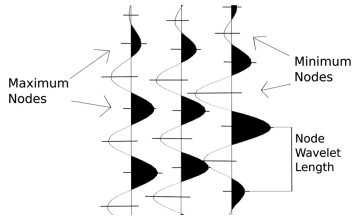
This software divides seismic traces into nodes (data points on a larger network), with a time parameter located at the relative maximum and minimum amplitudes of each trace (Fig. 1). These nodes contain information relative to their wavelet length (distance in time between the two neighboring nodes in the same trace), amplitude and position in time. It is important to emphasize that the software considers all the existing maximum and minimum points as a possible reflector, which makes it very sensitive to the processing steps (e.g., filters and gains) that the data has been previously submitted to. Each node is then compared to the nodes in the adjacent traces on both sides, using the difference between wavelets length, amplitude and time, in order to verify if there is enough similarity to establish a connection representing a possible real sedimentary structure. After the original data is submitted to the SI, a new .segy file is generated, which will be opened in SU for visualization of the result.

The following entries are necessary to run SI:

• The converted grid of original data in floating point numbers (Data1);

• Size of the time search window, to define the range of time to search for similar nodes in neighboring traces (NFindWindow);

• Number of interpolated traces to be placed between each trace only for the final visualization (TC);

• Number of the original traces in the data (ntrac);

• Number of sampling points of each trace (ns).

Figure 1.
Illustration of how the nodes are defined in individual traces. Nodes are represented by the horizontal lines placed at every relative maximum or minimum point of each trace, containing the information of their respective wavelet length, amplitude and position in time.

Data = Automatic_Interpretation_Function (Data1, NFindWindow, TC, ntrac, ns);

The software was divided into functions, to be performed in sequence using the output of the previous function:

• MaxMinAmp: This function finds the time of the relative maximum and minimum values of each trace, through the numerical derivative of the original traces. Subsequently, a data structure is created, which stores the time and the amplitude of each maximum and minimum point;

• Estru_Mont/Estru_MontMin: Both functions assemble a structure in which each element has the information of a single node (Fig. 2). Estru_Mont, separates the maxima, Estru_MontMin, separates the minima. The following information of each node is stored in the structure:

  1. Wavelet length, calculated from the difference of time of each neighboring node in the same trace (Fig. 1);

  2. Amplitude, which is the maximum or minimum value;

  3. Position in time.

• Rel_Node: This routine compares each node of a trace with the nodes of the right and left neighboring traces, using the provided size of the time search window. The comparison is made by calculating the differences between the following parameters of neighboring nodes: 1) Amplitude of the node itself; 2) Amplitude of the nearest nodes in the same trace; 3) Wavelet length; 4) Position of the node in time. The results of this routine are added in the structure;

• Rank_Node: This stage is one of the most important of SI, because it determines which are the nodes of a neighborhood that are the most similar to the nodes of the central trace. Here, the nodes of the left and right neighborhood of a node in the central trace are ranked, according to the similarity of the four parameters of the previous item and the weight given to each of them. The function assembles the ranking by finding the smallest differences in the values of each parameter, punctuating with greater value the neighboring node that has more similarity. The weights given to each parameter are: (P _am = 4) Weight of amplitude of the node itself; (P _an = 4) Amplitude of the nearest nodes in the same trace; (P _l = 4) Wavelet length; (P _t = 10) Position of the node in time. For each neighboring node the value of the ranking (NRank _i ) is defined by Equation 3:

$\frac{P_{am}}{N_{{am}_i}}+\frac{P_{an}}{N_{{an}_i}}+\frac{P_l}{N_{l_i}}+\frac{P_t}{N_{t_i}}=NRank$ (3)

In which:

• i =  the neighboring node number;
• Nam_i , Nan _i , Nl_i and Nt _i =  the relative values of the differences of each parameter for each neighboring node, given by equations 4, 5, 6 and 7:

$\frac{D_{{am}_i}}{S_{{am}_{min}}}=N_{{am}_i}$ (4)

$\frac{D_{{an}_i}}{S_{{an}_{min}}}=N_{{an}_i}$ (5)

$\frac{D_{l_i}}{S_{l_{min}}}=N_{l_i}$ (6)

$\frac{D_t}{S_{t_{min}}}=N_{t_i}$ (7)

In which:

• Dam_i, Dan_i, Dl_i and Dt_i =  the modules of the difference of the values for each parameter in each node;
• Dam_min, Dan_min, Dl_min and Dt_min =  the minimum values of the module of the differences of all compared nodes, for each parameter.

Figure 2.
Data structure mounted in the Estru_Mont function. The node structure contains n traces, which contain m nodes, with the respective information of wavelength amplitude and position in time.

Weight distribution was reached after some tests and the values proposed demonstrated to be capable of finding the expected reflectors, but can be easily modified within the program, as needed.

• Def_Lines: Using the data structure formed in Rank_Node, the connections that all the nodes make with their neighbors are selected by connecting those ranked first in the previous analysis. That is, each node has a connection line to the right and to the left (if they have neighbors within the search window). The result of this function is a new structure (Fig. 3) where each column contains the connecting lines of two adjacent traces, which store the information of the connected nodes (wavelength, amplitude and position in time);

• Rem_Cross: This function works with the two previous structures formed by the maximum and minimum nodes that were submitted to the previous routines, comparing them and eliminating all the crossing lines of both structures. It should be noted that, in the same input structure, there may be two equal lines (double link lines), because the same connection between a node to the right and a neighbor to the left can be chosen by the inverse comparison, indicating a greater degree of coherence in this connection (Fig. 4A). Thus, in order to be completely eliminated, a line that is present twice in the structure must also have crossed twice the lines of the structure to which it is being compared. If it is crossed just once it becomes a single link line, which will also be preserved (Fig. 4B);

• Rem_Equal: Function that eliminates all equal lines in the structure, i.e., all the lines that still have double links are turned into single-link ones;

• Order_Lines: Function that orders the lines in time within the structure, according to the first node of each link;

• Rem_X: This is the only function that performs an operation based on a priori geological criteria, since it eliminates the possibility of “X” crossings, that is, of a single node with four different links. This is due to the fact that there are no sedimentary structures with this characteristic. If the routine encounters an “X” cross, the link with the longest time gradient is deleted. A visual example of the result of the routine after that function is given in Fig. 5;

• Add_Mark: At this stage, the line structure is analyzed in order to search for and mark with flags the lines that:

  1. Display continuity from right to left;

  2. Possess no connection to the left;

  3. Possess no connection to the right;

  4. Have three connections. The purpose of this routine is to facilitate the connection of curves that will later be formed by the program;

• Curves: At this point, the line structures with minimum and maximum nodes are reunited. A new data structure is formed, containing as elements only the curves interpreted and considered a reflector by the previous processes, each curve is formed by each one of the continuous connected lines (Fig. 5). In order to establish the connection and formation of curves, a recursive function (Mont_Curve) is used, which makes use of the flags added in Add_Mark in the input structures. Each curve of this structure has an array composed of information from the points of nodes that formed it. The information is:

  1. Trace;

  2. Time;

  3. Amplitude;

  4. Wavelet length;

  5. Marker to check whether it is the end or the beginning point of the curve;

• Curve_Interpolation: This function creates nodes by the interpolation between the original nodes of the curves for the improvement of final visualization. New nodes are added in the data with information of the linear interpolation of the parameters. The amount of new nodes to be added between the existing nodes is defined in the function entry;

• Add_Curves_Dat: In the last stage, the interpolated curves are added to a synthetic grid for visualization of the result in SU;

• In the final visualization of SI, every line (different of the connection lines previously described) with black or white color represents a curve. Each line is a recognized reflector. The black color represents the curves composed by maximum nodes and the white color by minimum nodes. The amplitude of the curves defines the intensity of the colors, so that the more intense the colors the larger the amplitude. The wavelets length is directly represented by the thickness of the lines.

Figure 3.
Form of the data structure mounted with the Def_Lines function. The lines structure contains n columns, which contain m lines, with the respective information of wavelet length amplitude and position in time of the two nodes in the respective line.

Figure 4.
(A) Structure of the connections before the Rem_Cross function. The continuous lines represent nodes that connect to each other reciprocally (double link), the dashed lines represent connections where only one node connects to the other (single link). The blue lines represent the connections between Minimum nodes, and the red ones, connections between Maximum nodes. (B) Structure of connections after the Rem_Cross function. Through this routine, the dashed lines that cross with each other are deleted, and the continuous lines that cross another line become dashed ones.

Figure 5.
Visualization of the result of the SI after the use of the function Rem_X. The continuous lines represent the recognized reflectors by the SI in the example data. Red lines are formed by nodes of maxima and blue lines by nodes of minima.

APPLICATION OF THE STANDARDIZED INTERPRETER AND EVALUATION OF PROCESSING ROUTINES

The ability of SI to find lateral continuities between adjacent traces can help the interpretation of seismic sections. SI can be run after each processing routine, such as frequency filter, gains and trace interpolator, in order to evaluate the lateral continuity and form of their resulting reflectors. Here, SI is applied to a real dataset and used to evaluate different processing workflows, by applying it after each processing routine. Evaluation of the routines is done by comparing the reflectors interpreted by the SI with the expected aspect of sedimentary features, as discussed in the Geological Aspects section.

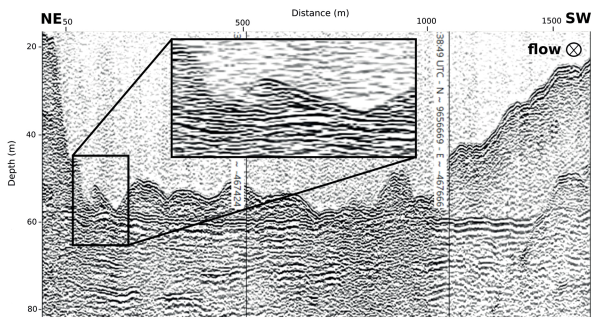
Application and evaluation of different processing routines is performed on a real dataset acquired employing a boomer source. The seismic cross-section images the bottom of the Amazon River (Fig. 6). First, unprocessed data is submitted to the SI. Later, the frequency filter routine is applied and then submitted to the SI to comparatively evaluate the results. The result of the frequency filter is also compared with the results obtained by a commercial software. Lastly, the AGC Gain and Trace Interpolation routines were used, both applied after the frequency filter. The results of these routines are compared with the frequency filter results, being also evaluated using the SI. To emphasize the effects of each processing routine, they were all applied to the same window of the section, which corresponds to a large subaqueous dune with internal structures.

Figure 6.
Seismic section processed with the frequency filter routine (300-1,300 Hz), using a commercial software. The data area chosen for the evaluation of the processing routines shows a dune within the frame cut.

Unprocessed data

The unprocessed data displayed in Fig. 7A, which was generated using SU software, served as a benchmark for successive processing stages. Depth was calculated considering a velocity of wave propagation of 1,500 m/s. As shown in Fig. 7A, even before any processing, the water-sediment interface is easily detected, whilst the internal reflectors representing sedimentary structures are not easily distinguishable. As the river bottom is easily recognizable, the SUXPICKER function was used to determine the interface in each trace for the application of the mute filter after the application of the frequency filter.

Figure 7.
(A) Unprocessed original data used to evaluate processing routines. (B) Image generated by the application of the SI on the unprocessed original data. The result of the SI evidences the difficulty in finding expected shapes of reflectors in the unprocessed image.

Application of SI on the unprocessed data evidences that the resulting form of the recognized lines do not have much lateral continuity and do not seem to correspond to expected sedimentary structures inside the dune (Fig. 7B), showing the need for a dedicated processing to enhance internal structures.

Frequency filter and Spectrum analyses

The Spectrum analysis shows the relative amplitudes of frequency ranges in the original data (Fig. 8). High amplitudes in frequencies below 300 Hz are common noises caused by secondary waves sources, such as the boat engine, which are usually removed. Above of 300 Hz, the spectrum shows two regions with high amplitude. One from 300 to 1,300 Hz (Region 1 in Fig. 8) and the other from 1,300 to 2,500 Hz (Region 2 in Fig. 8). In between, at around 1,500 Hz, there is a relative decrease of amplitude, separating the regions.

Figure 8.
The amplitude spectrum of the data, generated by the SUSPECFX function (amplitude × frequency - Hz), shows two regions with high energy that can be generated by the seismic source, one between 300 and 1,300 Hz (Region 1) and the other between 1,300 and 2,500 Hz (Region 2).

It is known that shallow seismic sources applied to aquatic environments can generate cavitation. In the boomer case, low-frequency waves caused by cavitation are described in the literature (Edgerton & Hayward 1964), and additional high frequency and high amplitude noise is known to result from the collapse of cavitation bubbles (Brennen 2005). Equipment specifications, provided by the manufacturer, report only its dominant frequency (1,200 Hz), and do not mention the operating frequency band. Thus, the relative decrease of amplitudes at 1,300 Hz might be related to a secondary source of higher frequency (Region 2 in Fig. 8). In this way, the usage of both regions with frequency peaks can generate a data superposition and result in misleading geological interpretation. In order to verify this possibility, the SI was applied after frequency filtering for three different bands:

• 300 to 1,300 Hz (Figs. 9A and 9B);

• 300 to 2,500 Hz (Figs. 10A and 10B);

• 1,300 to 2,500 Hz (Figs. 10C and 10D).

Figure 9.
(A) Seismic image after frequency filtering (SUFILTER) for a band of 300-1,300 Hz and mute filtering (SUMUTE). (B) Analysis of the result with the SI.

Figure 10.
Seismic image after filtering (SUFILTER and SUMUTE) and analysis of the result with the SI for two different frequency bands: (A) and (B), for with a band of 300-2,500 Hz; (C) and (D), for a band of 1,300-2,500 Hz.

Due to the reverberation artifacts that appear above the water-sediment interface after the frequency filter routine, the SUMUTE is applied, using the file generated in the previous step.

The application of SI in the data with the frequency filter band of 300-1,300 Hz resulted in lines with a significant lateral continuity, being more similar to the expected reflectors to be found within a dune, such as inclined planar reflectors related to planar cross stratification, concave-up reflectors that represent trough cross stratification and reflectors of greater amplitude and continuity related to cross-strata set boundaries (Fig. 9B). Application of SI in the data with a band of 300-2,500 Hz resulted in lines with less lateral continuity, hampering recognition of sedimentary structures in the data (Fig. 10A). Finally, application of SI in the data with a band of 1,300-2,500 Hz resulted in lines with some lateral continuity and attenuated amplitudes, being also thinner compared to data with 300-1,300 Hz, due to high frequencies of the filtering (Fig. 10D). These results evidence that sources with different frequency bands can display very different reflectors (Figs. 9B and 10D), so that when two bands with high amplitude are filtered and put together, the result can be more difficult to interpret, due to the superposition of data (Fig. 10B). As the dominant frequency of the equipment is 1,200 Hz, the most probable band with high amplitude that is not generated by cavitation noises is the 300-1,300 Hz, thus being the frequency used in this work. In this way, the SI shows that the frequency filter is a very relevant routine, since after processing, the interpretation software presented features more similar to the expected internal structures than when applied in data without processing (Fig. 7B).

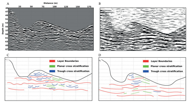
Moreover, these results obtained by open-access software (SU and SI) were compared to the ones from a commercial software. Figure 11 displays data from the open-access software used in this work (Fig. 11A) and from the commercial software (Fig. 11B) after applying the same band-pass filter (300-1,300 Hz). Comparison evidences that the open-access software delivers a result at least as good as the commercial software. The open-access software presents high resolution results, allowing accurate interpretation of sedimentary structures. Additionally, the open-access software displays thinner ondulated reflectors (Fig. 11C) in areas where the commercial software displays thick and straight reflectors (Fig. 11D). Open-access software also displayed reflectors with a great continuity, highlighting connections otherwise not observable.

Figure 11.
Comparison of the SI result with a commercial software. (A) Result of SI after the frequency filtering (same as Fig. 9B); (B) data processed with a commercial software, only with frequency filtering with a band of 300-1,300 Hz (same as Fig. 6-inset); (C) geological interpretation of Fig 11A. Recognized structures. Red: Layer boundaries; Blue: Trough cross stratification; Green: Planar cross stratification; (D) Geological interpretation of Fig 11B.

AGC Gain

AGC gain is used after the frequency filter (Fig. 12A), with a gain window of 0.01 seconds (wagc = 0.01) and gagc mode (Gaussian window), resulting in more evident reflectors. The result of the SI applied after AGC gain (Fig. 12B) shows curves with similar forms compared to the results of frequency filter (Fig. 12C), and of the SI used after (Fig. 12D), but the apparent amplitude of the curves is normalized, leading to enhanced reflectors but also increased background noise. Additionally, AGC gain does not preserve the relative amplitude of each reflector, thus losing useful information about impedance contrasts, in this case of application related to grain-size variation. For instance, analysis of wavelets amplitudes in seismic reflection data acquired with boomer has been used to find sedimentary layers rich in gas (e.g., Baltzer et al. 2005, Cooper & Hart 2002). Because of that, the use of AGC gain is suggested as an optional step of processing to help in geological interpretation, depending on the dataset and the features to be imaged.

Figure 12.
Comparison of the three evaluated routines of frequency filter (300-1,300 Hz), AGC gain and Traces Interpolator, followed by the application of SI. (A) Image after frequency filter and AGC gain; (B) Interpretation by SI after AGC gain; (C) Image after the application of the frequency filter routine; (D) Interpretation of the data made by SI after the frequency filter; (E) Image after frequency filter and applying the interpolation routine; (f) Interpretation by SI after the interpolation routine.

Trace Interpolation routine

The Traces Interpolation routine, developed in GNU Octave, is applied to the data after the frequency filter (Fig. 12E). Four new traces were added between the original traces by interpolation, after that, each trace was replaced two times by the interpolation with its two closest neighbors. Compared to the results of the frequency filter, this process smoothed the form of the reflectors, especially the more horizontal ones. In submitting the data to the SI (Fig. 12F), a very large correspondence was observed in the forms of the curves with the result of the Traces Interpolation before the application of the SI (Fig. 12E). This is explained by the fact that the traces added by the Traces Interpolator are not real and bear much resemblance to their neighbors. This result shows that the interpolation is also a type of interpretation.

CONCLUSION

The SI software here presented with a source code written in GNU Octave that finds the best linkage between individual traces in seismic sections (SI) proved to be a valid process to help in geological interpretation and enabled the objective evaluation of different processing routines, aiming at the visualization of internal sedimentary structures in shallow seismic data. The SI reduces the bias of geological interpretation and enables the proposition of a dedicated processing flowchart for seismic data obtained by a boomer source in fluvial environments. Routine evaluation with the SI showed that:

• frequency filtering proved to be essential because the information of interest is in a well-defined frequency range;

• AGC gain routine has the advantage of assisting in the recognition of reflector forms, however, it masks useful information, such as the acoustic impedance contrasts of sedimentary structures;

• the Trace Interpolator resulted in a smoother image, in some ways easier to interpret.

Thus, applying AGC gain and data interpolation might be useful depending on the sort of information that is necessary for the specific objectives of each survey. The proposed flowchart leads to good results, revealed by the SI in the form of linked surfaces clearly related to common sedimentary structure geometries.

Apart from being useful as an unbiased tool for the evaluation of processing routines, the SI proved to be helpful in geological interpretation itself, since it facilitates the visualization of the form of the reflectors, serving as an intermediate stage between the processing and the geological interpretation. In addition, its application is theoretically possible in any geophysical data in .segy format.

ACKNOWLEDGMENTS

This research had the support from grant “Dimensions US-Biota-São Paulo: Assembly and evolution of the Amazon biota and its environment: an integrated approach”, co-funded by Fundação de Amparo à Pesquisa do Estado de São Paulo (2012/50260-6, 2014/16739-8, 2016/03091-5), US National Science Foundation (NSF DEB 1241066), and the National Aeronautics and Space Administration (NASA). Additional support from Fundação de Amparo à Pesquisa do Estado de São Paulo was in the form of scholarships ­(2017/06874-3, 2018/02197-0). We also thank the scholarships granted by CAPES (PROEX-558/2011) to L. M. Tamura, and by CNPq to R. P. Almeida (305218/2009-3). Sub-bottom seismic profiling (boomer) was acquired by SALT Sea and Limno Technology.

REFERENCES

• Almeida R.P., Galeazzi C.P., Freitas B.T., Janikian L., Ianniruberto M., Marconato A. 2016. Large barchanoid dunes in the Amazon River and the rock record: Implications for interpreting large river system. Earth Planet Science Letters, 454:92-102. https://doi.org/10.1016/j.epsl.2016.08.029
  » https://doi.org/10.1016/j.epsl.2016.08.029
• Baltzer A., Tessier B., Nouzé H., Bates R., Moore C., Menier D. 2005. Seistec Seismic Profiles: A Tool to Differentiate Gas Signatures. Marine Geophysical Research, 26(2-4):235-245. https://doi.org/10.1007/s11001-005-3721-x
  » https://doi.org/10.1007/s11001-005-3721-x
• Bond C.E., Gibbs A.D., Shipton Z.K., Jones S. 2007. What do you think this is? “Conceptual uncertainty” in geoscience interpretation. GSA Today, 17(11):4-10. https://doi.org/10.1130/GSAT01711A.1
  » https://doi.org/10.1130/GSAT01711A.1
• Borgos H.G., Skov T., Randen T., SØnneland L. 2003. Automated geometry extraction from 3D seismic data. SEG Expanded Abstracts, 22:1541-1544. https://doi.org/10.1190/1.1817590
  » https://doi.org/10.1190/1.1817590
• Brennen C.E. 2005. Fundamentals of multiphase flow Cambridge, Cambridge University Press, 410 p.
• Bridge J.S., Demicco R. 2008. Earth Surface Processes, Landforms, and Sediment Deposits Cambridge, Cambridge University Press.
• Cooper A.K., Hart P.E. 2002. High-resolution seismic-reflection investigation of the northern Gulf of Mexico gas-hydrate-stability zone. Marine and Petroleum Geology, 19(10):1275-1293. http://dx.doi.org/10.1016/S0264-8172(02)00107-1
  » http://dx.doi.org/10.1016/S0264-8172(02)00107-1
• Edgerton H.E., Hayward G.G. 1964. The “boomer” sonar source for seismic profiling. Journal of Geophysical Research, 68(14):3033-3042. https://doi.org/10.1029/JZ069i014p03033
  » https://doi.org/10.1029/JZ069i014p03033
• Kumar P.C., Sain K. 2018. Attribute amalgamation-aiding interpretation of faults from seismic data: An example from Waitara 3D prospect in Taranaki basin off New Zealand. Journal of Applied Geophysics, 159:52-68. http://dx.doi.org/10.1016/j.jappgeo.2018.07.023
  » http://dx.doi.org/10.1016/j.jappgeo.2018.07.023
• Maraio S., Bruno P.P.G., Picotti V., Mair V., Brardinoni F. 2018. High-resolution seismic imaging of debris-flow fans, alluvial valley fills and hosting bedrock geometry in Vinschgau/Val Venosta, Eastern Italian Alps. Journal of Applied Geophysics, 157:61-72. http://dx.doi.org/10.1016/j.jappgeo.2018.07.001
  » http://dx.doi.org/10.1016/j.jappgeo.2018.07.001
• Nichols G. 2009. Sedimentology and Stratigraphy 2ª ed. Oxford, Blackwell, 53-56 p.
• Orlando L., Contini P., de Girolamo P. 2017. Seismic scattering attribute for sedimentary classification of nearshore marine quarries for a major beach nourishment project: Case study of Adriatic coastline, Regione Abruzzo (Italy). Journal of Applied Geophysics, 141:1-12. http://dx.doi.org/10.1016/j.jappgeo.2017.04.004
  » http://dx.doi.org/10.1016/j.jappgeo.2017.04.004
• Shafiq M.A.S., Di H., AlRegib G. 2018. A novel approach for automated detection of listric faults within migrated seismic volumes. Journal of Applied Geophysics, 155:94-101. https://doi.org/10.1016/j.jappgeo.2018.05.013
  » https://doi.org/10.1016/j.jappgeo.2018.05.013
• Souza L.A.P. 2006. Revisão crítica da aplicabilidade dos métodos geofísicos na investigação de áreas submersas rasas PhD Thesis, Instituto Oceanográfico, Universidade de São Paulo.
• Steeples D.W. 2000. A review of shallow seismic methods. Annali di Geofisica, 43(6):1021-1044. https://doi.org/10.4401/ag-3687
  » https://doi.org/10.4401/ag-3687

• Manuscript ID: 20180121.

Publication Dates

• Publication in this collection
  29 Apr 2019
• Date of issue
  2019

History

• Received
  01 Nov 2018
• Accepted
  20 Mar 2019