Uncertainty estimation in hydrodynamic modeling using Bayesian techniques

Estimação de incertezas na modelagem hidrodinâmica por meio de técnicas Bayesianas

ABSTRACT

Uncertainty estimation analysis has emerged as a fundamental study to understand the effects of errors inherent to hydrodynamic modeling processes, of aleatory and epistemic nature, due to input data such as discharge, topography and bathymetry, to the structure and parameterization of the mathematical models used and to their necessary boundary and initial conditions. The study reported in this paper sought to apply a Bayesian-based methodology, associated with thousands of Markov Chain Monte Carlo simulations, in order to identify and quantify the uncertainty related to the Manning’s n roughness coefficient in a 1D hydrodynamic model and the total uncertainty involved in the prediction of hydrographs and water surface elevation profiles resulting from flood routing through a reach located in the upper São Francisco river, between the Abaeté river outlet and the town of Pirapora. The results show that the Bayesian scheme allowed an adequate posterior identification of the parametric uncertainties and of those associated to other sources of errors, with important changes in the prior probability distributions. In addition, the residuals analysis corroborates the applicability of the method to the analysis of uncertainties in hydrodynamic modeling through the use of a more flexible likelihood function than the classical one based on the hypotheses of normality, homoscedasticity and uncorrelated residuals. Future work includes the sensitivity evaluation of the posterior distributions to the addition of lateral inflows, especially concerning the residuals serial correlation, as well as the adoption of other variables to update the prior uncertainties, and the validation of the methodology through the use of the posterior distributions to estimate the total uncertainty involved in the prediction of floods other than the ones used in the inference process.

Keywords:
Uncertainty estimation; Hydrodynamic models; Bayesian inference; Markov chain Monte Carlo simulation; Probabilistic flood inundation maps

RESUMO

A avaliação de incertezas tem emergido como estudo primordial para se conhecerem os efeitos dos erros inerentes aos processos de modelagem de perfis de escoamento de vazões de cheia, de natureza aleatória e epistêmica, presentes em dados de entrada como vazões e topobatimetria, na estrutura e parametrização dos modelos matemáticos utilizados e nas suas necessárias condições de contorno e iniciais. Dessa forma, o estudo reportado neste artigo buscou aplicar uma metodologia de cunho Bayesiano, associada a milhares de simulações de Monte Carlo por Cadeias de Markov, a fim de identificar e quantificar a incerteza inerente ao coeficiente de rugosidade de Manning de um modelo hidrodinâmico unidimensional e a incerteza total envolvida na predição de hidrogramas e profundidades resultantes da propagação de cheias por um trecho do Alto rio São Francisco, entre a foz do rio Abaeté e a cidade de Pirapora. Os resultados mostram que o esquema Bayesiano permitiu uma adequada identificação a posteriori das incertezas paramétricas e associadas às demais fontes de erros, com alteração importante das distribuições de probabilidade estipuladas a priori. Ademais, a análise estatística dos resíduos da modelagem veio corroborar a aplicabilidade do método à análise de incertezas na modelagem hidrodinâmica por meio do uso de uma função de verossimilhança mais flexível do que a clássica função baseada nas hipóteses de normalidade, homoscedasticidade e ausência de correlação serial para os resíduos. A continuidade deste trabalho prevê ainda a avaliação de sensibilidade das incertezas a posteriori à inserção de afluências laterais, sobretudo no que tange à correlação temporal dos resíduos, bem como a adoção de outras variáveis como informação de atualização das incertezas, e a validação da metodologia por meio do uso das incertezas a posteriori para estimação da incerteza total envolvida na predição de outros eventos de cheia que não tenham sido utilizados no processo de inferência.

Palavras-chave:
Estimação de incertezas; Modelos hidrodinâmicos; Inferência Bayesiana; Simulações de Monte Carlo por Cadeias de Markov; Mapas de inundação probabilísticos

INTRODUCTION

The evaluation of floods and inundations, and their effects on riverine populations, has been the object of study by water resources engineers worldwide. Numerical models of hydraulic and hydrologic simulation have advanced greatly in the last two decades, which is partially due to the increase of computational data processing capacity and the possibility of acquiring accurate topographic bases in many parts of the globe, especially in the United States and European countries. Despite the improvements made in the technical and data acquisition fields, and the efforts of many governments and agencies at local and federal scales, to prevent and control floods and their impacts, some studies indicate that the associated damages continue to increase (MERWADE et al., 2008). In Brazil, it is estimated that the economic losses caused by floods amount to between US $ 1 billion and US $ 2 billion per year (MILOGRANA, 2009). Thus, reducing losses, more accurately forecasting affected areas, and disseminating pertinent information for civil defense, planning agencies, and for the overall public, become essential activities for mitigating and reducing the effects of flooding on riverine populations in urban and rural areas, as well as on the local economy (MERWADE et al., 2008).

Advances and improvements in models and in the quality and quantity of input data, as well as the increasing need to understand, control and mitigate floods and their effects, have opened up new research and opportunities for the water resources sector. Some of the new challenges are: (i) the importance of dealing with equifinality, or the possibility of obtaining model outputs with comparable adjustment qualities from different, and sometimes numerous, possible combinations of parameters (BEVEN, 2006); (ii) the definition of the degree of refinement and complexity required for a model to have a reasonable or acceptable physical response from the point of view of hydrological and hydraulic realism (DI BALDASSARRE et al., 2010); (iii) the need of quantifying uncertainties or errors associated with input data, parameters and model structure (MERWADE et al., 2008); (iv) the estimation of how the aforementioned information influences each other and contributes to total uncertainty (JUNG; MERWADE, 2012, 2015); (v) the quantification of predictive uncertainty, which means the errors involved in predicting output variables as estimated by models (TODINI, 2007); and (vi) the attribution of probabilities to the individual results provided by models, replacing the commonly adopted deterministic approach (MERWADE et al., 2008).

In this paper, we intend to seek alternatives to the issues (iii), (v) and (vi) above mentioned, in order to understand the reliability and limitations of a hydrodynamic model widely used in the national and international technical and academic fields, powered by topobathymetric, discharge and stage data commonly available in Brazil and other countries.

In a great retrospective compilation on advances and challenges of hydrologic and hydraulic modeling focused on flood studies and flood inundation mapping, Merwade et al. (2008) argued that the uncertainty quantification would be one of the central points to be urgently studied in the following years by the community of water resources engineers. After 10 years of this compilation, there is a relevant amount of studies in this field concentrated on rainfall-runoff transformation (STEDINGER et al., 2008; VRUGT et al., 2008a, 2008b), supplied by numerous examples developed in previous years (see, for example, the compilation of BEVEN; BINLEY, 2014). Hydraulic modeling, in steady or unsteady regimes, on the contrary, has presented a modest number of examples (CAMACHO et al., 2015). In this case, the methods based on the theory of probability for uncertainty representation prevail (HALL, 2003), as well as those of approximate nature. These two aspects are characteristic of situations in which it is not possible to obtain analytical solutions to quantify either the uncertainty associated with each one of the components of an environmental system model (such as input and output, parameters and model structure), which is generally non-linear in nature, or the predictive uncertainty. Among the techniques with such attributes, those having wide applicability in hydrologic and hydraulic modeling are the ones based on Monte Carlo experiments (CAMACHO et al., 2015) and on updating the prior knowledge on the uncertainties of each component of an environmental system model through Bayes’s theorem (AYYUB; KLIR, 2006; HUTTON et al., 2011).

In regard to the hydraulic and hydrodynamic modeling focused on flood inundation water surface profile definition and mapping, the uncertainties are due to a number of aspects that are inherent to the structure of models, their parameters and input data, among which the most relevant are:

• Design peak discharge or design flood hydrograph, which are estimated either by local or regional frequency analysis, or regional regression curves based on basin physical features, or rainfall-runoff modeling. Such techniques add uncertainties due to factors such as inaccurate or ill-defined rating curves, few streamflow measurement data available for its calculation and lack of flood stage records. When a hydrologic model is used, the main sources of errors are due to rainfall data acquisition procedures and methods for rainfall spatial interpolation, rainfall time distribution, and the uncertainties arisen from model parameters estimation (MERWADE et al., 2008);

• Topographic and bathymetric data for hydrologic and hydraulic models and their treatment for insertion in modeling, whose uncertainties can be attributed to the spatial resolution and to the vertical accuracy of the information, and to the different methods available for spatial interpolation of the raw data to generate digital terrain models (MDTs) or digital elevation models (MDEs) (COOK; MERWADE, 2009);

• Hydraulic modeling itself, which adds uncertainty due to: the parameters, especially the roughness; the number of dimensions considered (1D, 2D or 3D), the representation of the main channel; the numerical method adopted for solving the hydrodynamic flow equations; the mesh or grid quality (whether 2D or 3D) or the cross sections spacing (if 1D); and the representation of boundary conditions upstream and downstream of structures such as bridges, levees and culverts (PAPPENBERGER et al., 2005; HUTTON et al., 2011); and

• If the main goal is the development of flood inundation maps, then errors due to the different techniques and algorithms used in the flood extension generation defined from model output are added up (MERWADE et al., 2008).

Jung and Merwade (2012, 2015) pointed out the uncertainty estimation involved in hydrodynamic modeling as a tool to aid in the detection of variables and data that require greater improvement in terms of acquisition, calculation or treatment (such as topographic data and regional equations to obtain design floods), in order to reduce their contribution to total uncertainty.

Moreover, the propagation of the uncertainties attributed to different sources of errors in modeling through the respective model allows the quantification of the total uncertainty associated with possible future values of output variables, both for forecasting and prediction, called predictive uncertainty (TODINI, 2007; STEDINGER et al., 2008; SCHOUPS; VRUGT, 2010). When it comes to hydraulic and hydrodynamic modeling, predictive uncertainty characterizes the impact of uncertainties on discharge and stage hydrographs along the river reach of interest, and on flood inundation areas, the arrival time of a flood wave and on the velocity variation in the main channel and floodplains.

In several studies of uncertainty estimation in hydraulic and hydrodynamic modeling focused on flood inundation mapping, the predictive uncertainty associated with a design flow has been represented in the form of a probabilistic flood map (PAPPENBERGER et al., 2005, 2006; DI BALDASSARRE et al., 2010; BEVEN et al., 2011; JUNG; MERWADE, 2012). In such a situation, the contours depict floodplain areas with greater or lesser chances of being reached than others, given the same design flow, due to uncertainties in data, parameters and equations that are involved in flood simulation and forecasting.

Finally, some studies exemplify how to represent the predictive uncertainty associated with hydraulic and hydrodynamic modeling on flood hazard maps, (PAPPENBERGER et al., 2006), as well as on functions defined to support decision making process and flood warning in the occurrence of extreme floods (TODINI, 2007).

The Bayesian approach applied to the uncertainty estimation

Among the several methods that emerged in the last decades aimed at quantifying uncertainties in models used in several areas of knowledge, those of Bayesian approach find examples in hydrology, hydraulics and hydrogeology (HUTTON et al., 2011; VRUGT, 2016). Generally speaking, these methods allow the combination of the initial knowledge about the variability of parameters and variables involved in modeling with one or more sets of systematic observations of a phenomenon associated with them (HUTTON et al., 2011). Part of the explanation that follows was adapted from Vrugt (2016) and is focused on the model parameters in a similar fashion to several studies (PAPPENBERGER et al., 2005; BLASONE et al., 2008; The SCHOUPS; VRUGT, 2010; SILVA et al., 2014; CAMACHO et al., 2015). In the following paragraphs, the expression “probability density function” is replaced by the abbreviation PDF.

Consider that $\tilde{Y}=\left\{\widetilde{y_1},\cdots ,\widetilde{y_n}\right\}$ is a discrete vector of measurements, or observations, of a certain phenomenon (e.g. flow in a gauged river cross section) at times $t=\left\{\mathrm{1,}\cdots ,n\right\}$ that summarizes the response of certain environmental system $\Im$ due to observed input data $\tilde{X}=\left\{{\tilde{x}}_1,\cdots ,{\tilde{x}}_n\right\}$. In a simplified way, observations are associated with this physical system through the following relationship:

$\tilde{Y}\leftarrow \Im \left(\theta \right)+\epsilon$ (1)

where $\theta =\left\{{\theta }_1,\cdots ,{\theta }_d\right\}$ represents a parameter vector and $\epsilon =\left\{{\epsilon }_1,\cdots ,{\epsilon }_n\right\}$ is a n-vector of residuals (i.e. errors).

Having a mathematical model to explain the physical process in question, it can be represented by the generic expression:

$$\tilde{Y}\leftarrow \mathcal{F}\left(\theta ,\widetilde{X,}\widetilde{{\phi }_0}\right)+E=Y\left(\theta ,\widetilde{X,}\widetilde{{\phi }_0}\right)+E$$ (2)

where $\widetilde{{\phi }_0}$signifies the initial conditions; $E=\left\{e_1,\cdots ,e_n\right\}$ includes errors in observed data (both in input, $\tilde{X}$, and output variables, $\tilde{Y}$), as well as errors inherent to the $\mathcal{F}$ model itself and its parameterization θ; and $Y\left(\theta ,\widetilde{X,}\widetilde{{\phi }_0}\right)=\left\{y_1,\cdots ,y_n\right\}$ is the output vector simulated by the model.

The problem synthesized by equations 1 and 2 can be analyzed through a Bayesian approach, in which the posterior joint PDF of parameters “can be derived by conditioning the spatio-temporal behavior of the model on measurements of the observed system response” (VRUGT, 2016). In other words, the resulting probability distribution expresses the uncertainty associated with the model parameters, previously represented by the prior knowledge, which has been updated using the available information. Formally, these concepts may be represented by the Bayes’s theorem, adapted to the uncertainty estimation, as shown in Equation 3:

$\text{p}\left(\theta |\tilde{Y}\right)=\frac{\text{p}\left(\theta \right)·\text{p}\left(\tilde{Y}|\theta \right)}{\text{p}\left(\tilde{Y}\right)}$ (3)

where $\text{p}\left(\theta \right)$ and $\text{p}\left(\theta |\tilde{Y}\right)$ represent, respectively, the prior and the posterior joint PDFs of the model parameters, and $\text{p}\left(\tilde{Y}|\theta \right)\equiv \text{L}\left(\theta |\tilde{Y}\right)$ denotes the likelihood function. The evidence represents the prior joint predictive PDF, which operates as a normalizing constant (scalar) such that the posterior distribution integrates to unity. In practice, $\text{p}\left(\tilde{Y}\right)$ is not required for posterior estimation, since all statistical inferences about $\text{p}\left(\theta |\tilde{Y}\right)$ can be made from the unnormalized probability density below (KAVETSKI et al., 2003; CAMACHO et al., 2015; VRUGT, 2016):

$\text{p}\left(\theta |\tilde{Y}\right)\propto \text{p}\left(\theta \right)·\text{L}\left(\theta |\tilde{Y}\right)$ (4)

The concept expressed in Equation 4 is widely employed in order to quantify parametric uncertainty and propagate it through the model in order to calculate predictive uncertainty. Kavetski et al. (2003) have proposed an adaptation from this classical formulation to allow the separation of the uncertainties due to input data errors of those arising from errors of the parameters in a rainfall-runoff modeling.

Based on these initial concepts, four basic elements are necessary to implement the Bayesian approach in order to quantify modeling uncertainties, as pointed out by Hutton et al. (2011):

• Definition of the content of the prior information, expressed by means of theoretical prior probability distributions for each one of the model parameters;

• Choice of an appropriate error model, which consists of assumptions about the expected behavior of the residuals vector $E$, as well as the theoretical probability distribution that best represents them;

• Deduction of an appropriate likelihood function, starting from the hypothesized error model; and

• Analytical deduction of the posterior joint PDF, whenever possible, or application of numerical methods for its estimation, which is the case in most practical situations in environmental system modeling (HUTTON et al., 2011; BOZZI et al., 2015).

The prior probability distribution may be non-informative or informative. In the first case, non-informative distributions are used, which conceptually demonstrate the vague prior knowledge about the parameters or represent the expectation that the information provided by observed data might exceed the prior content of parameters (FERNANDES; SILVA, 2017). For this purpose, several authors consider the uniform distribution with lower and upper limits that express the plausible values range of a given variable or parameter (PAPPENBERGER et al., 2005; VRUGT et al., 2008a; SCHOUPS; VRUGT, 2010; JUNG; MERWADE, 2012). The Gamma distribution with small scale parameter may be used to prescribe a rigorously formal non-informative distribution with unlimited θ (FERNANDES; SILVA, 2017).

In the second case, an informative distribution should be elicited, thus reflecting the previous knowledge about the evaluated variable or parameter. Distributions such as the Normal (truncated or not), Beta, Gamma or Triangular may be applied, as reported by Kavetski et al. (2006) and Bozzi et al. (2015).

In turn, the likelihood function$\text{L}\left(\theta |\tilde{Y}\right)$ can be interpreted as a metric that summarizes the differences between the model simulations and the corresponding observations (i.e. errors, or residuals). In other words, it is summarized in most cases by a probabilistic expression that denotes the functional relation between output data and $\theta$, and thus indicates the overall behavior assumed for the residuals. This is the reason why its definition depends directly on the so-called error model, as defined by Kavetski et al. (2006), Schoups and Vrugt (2010) and Hutton et al. (2011). It does not need to be properly represented by a PDF - which in turn defines whether the method is formally Bayesian or not (STEDINGER et al., 2008; HUTTON et al., 2011; VRUGT, 2016). A widely adopted hypothesis is that the residuals $E\left(\theta \right)=\tilde{Y}-Y\left(\theta \right)=\left\{e_1\left(\theta \right),\cdots ,e_n\left(\theta \right)\right\}$ are free from autocorrelation, in which case the likelihood function can be expressed by Equation 5:

$\text{L}\left(\theta |\tilde{Y}\right)={\text{f}}_{\widetilde{y_1}}\left(y_1\left(\theta \right)\right)\times \cdots \times {\text{f}}_{\widetilde{y_n}}\left(y_n\left(\theta \right)\right)={\displaystyle \prod }_{t=1}^n{\text{f}}_{\widetilde{y_t}}\left(y_t\left(\theta \right)\right)$ (5)

where ${\text{f}}_a\left(b\right)$ denotes the PDF of $a$ evaluated at $b$ (VRUGT, 2016). Depending on the assumptions made about the model residuals, expressions ${\text{f}}_a\left(b\right)$ are deduced to obtain likelihood functions applicable to different environmental systems. For example, if it is assumed that the residuals are normally distributed, e.g. $e_t\left(\theta \right)~\mathcal{N}\left(\mathrm{0,}{\widehat{\sigma }}_t^2\right)$, then Equation 5 becomes:

$\text{L}\left(\theta |\widetilde{Y,}{\widehat{\sigma }}_{}^2\right)={\displaystyle \prod }_{t=1}^n\frac{1}{\sqrt{2\pi {\widehat{\sigma }}_t^2}}·\text{exp}\left[-\frac{1}{2}·{\left(\frac{\widetilde{y_t}-y_t\left(\theta \right)}{\widehat{{\sigma }_t}}\right)}^2\right]$ (6)

where $\widehat{\sigma }=\left\{\widehat{{\sigma }_1},\cdots ,\widehat{{\sigma }_t}\right\}$ is a vector of the standard deviations of errors contained in observations (when compared to simulation outputs). Equation 6 allows consideration of homoscedasticity (constant variance) or heteroscedasticity (variance depending on the information magnitude). Variables associated with residuals, such as those of vector $\widehat{\sigma }$, may be inferred along with the parametric vector $\theta$, in circumstances in which a posterior estimation from the error series is not possible or even when the objective is to quantify its uncertainties in a similar fashion to the ones performed for the model parameters. They are generally assigned to error model parameters (SCHOUPS; VRUGT, 2010) or latent or nuisance variables (KAVETSKI et al., 2003, 2006; VRUGT, 2016).

For reasons of numerical stability and algebraic simplicity, it is convenient to work with the log-likelihood function. Thus, Equation 6, for example, takes the format of Equation 7:

$\text{L}\left(\theta |\widetilde{Y,}{\widehat{\sigma }}_{}^2\right)=-\frac{n}{2}·\text{log}\left(2\pi \right)-{\displaystyle \sum }_{t=1}^n\left\{\text{log}\left(\widehat{{\sigma }_t}\right)\right\}-\frac{1}{2}·{\displaystyle \sum }_{t=1}^n{\left(\frac{\widetilde{y_t}-y_t\left(\theta \right)}{\widehat{{\sigma }_t}}\right)}^2$ (7)

which can be reduced to Equation 8 (KAVETSKI et al., 2003):

$\text{L}\left(\theta |\tilde{Y}\right)\propto -\left(\frac{n-1}{2}\right)·\text{log}\left\{{\displaystyle \sum }_{t=1}^n{\left(e_t\left(\theta \right)\right)}^2\right\}$ (8)

if the errors are homoscedastic. In this case, the variance can be estimated, after Bayesian inference, using Equation 9 (KAVETSKI et al., 2003):

${\sigma }^2\approx \frac{1}{n}·{\displaystyle \sum }_{t=1}^n{\left[e_t\left(\widehat{\theta }\right)\right]}^2$ (9)

in which $\widehat{\theta }$ is the mode of the posterior parametric vector estimate.

Equation 8 is the most adopted likelihood function in uncertainty assessment studies associated with rainfall-runoff transformation or hydrodynamic models that have used the formal Bayesian approach (KAVETSKI et al., 2003; VRUGT et al., 2003, 2008a; CHENG et al., 2014; CAMACHO et al., 2015).

However, the correct prescription of the error model, and, consequently, of the likelihood function, remains one of the major challenges of the Bayesian approach applied to the study of uncertainties, since most modeled physical processes have nonlinear behavior and show autocorrelated, heteroscedastic and non-Gaussian modeling residuals (KAVETSKI et al., 2003; SCHOUPS; VRUGT, 2010). Thus, the adoption of likelihood functions similar to equations 7 and 8 may lead to poor, incorrect estimation of the posterior joint PDF (KAVETSKI et al., 2003; HUTTON et al., 2011).

Due to this standoff, several studies of likelihood functions evaluation were carried out to define expressions with the ability to adequately characterize the above conditions for the residuals (SCHOUPS; VRUGT, 2010; SMITH et al., 2010; SCHARNAGL et al., 2015), at the cost of adding some variables related to them. This aspect certainly resulted in more complexity to the Bayesian estimation process and in the possibility of better identification of the uncertainties associated with the modeling parameters, in addition to the perspective of being able to represent, albeit implicitly, the structural uncertainties and those associated with input and output data (STEDINGER et al., 2008; HUTTON et al., 2011).

Once the prior PDFs and the likelihood function have been defined, the posterior joint PDF estimation of the parameters of the model and also of those related to the residuals, when applicable, is then estimated. Due to the nonlinear nature of most real systems and their models, this task becomes impractical through the use of equations or analytical approximations (VRUGT, 2016). Thus, iterative methods based on Monte Carlo simulations (MC) are generally used for generating posterior distribution samples and obtaining their statistical descriptors.

Classic Monte Carlo simulation methods are based on generating thousands of samples from the prior PDFs. Although already widely used, they have been shown to be ineffective both in exploring higher order multidimensional parametric spaces and in situations of incorrect prescription of the prior PDFs (HUTTON et al., 2011).

The major shortcoming of MC simulations is that information from the model sampling procedure at each run is not used to improve exploration of the HPD – High Probability Density – region of parameter space (HUTTON et al., 2011). As a way to overcome this limitation, techniques based on Markov Chain Monte Carlo (MCMC) simulations emerged about 70 years ago (METROPOLIS et al., 1953; HASTINGS, 1970), based on the generation of a random walk through parametric space that progressively reaches a stationary distribution representing the target distribution, which, in the case of Bayesian techniques, can be considered as a posterior joint distribution. Using some objective criterion to perform the jumps between successive iterations in a chain, guided by the so-called proposed distribution, a sample of parameters is generated from the target distribution, and assigned to an acceptance probability, thus defining whether the current state of the chain should be used to evolve to the next step, or if it should be done from the previous state.

MCMC techniques have evolved over the last decades to accelerate chain convergence toward stationary distribution, and to ensure the applicability of the method to high dimensional models. Among the most recent advances, two algorithms are mentioned: Differential Evolution Markov Chain or DE-MC (TER BRAAK, 2006 apud VRUGT, 2016), and Differential Evolution Adaptive Metropolis or DREAM (VRUGT et al., 2008a, 2008b, 2009). Vrugt (2016) presents a retrospective compilation of the most important MCMC algorithms, the main differences among them and the improvements provided by each one.

Regarding the hydraulic modeling of floods, in steady or unsteady regimes, the studies of uncertainty quantification that use informal likelihood functions prevail, this being the reason why they are called pseudo-Bayesian methods. These functions are based on performance measures commonly used in hydrologic and hydraulic modeling, involving the differences between simulated and observed values ​​of the output variables (discharge in the basin outlet or the downstream end of the river reach; depth and width in cross sections; flood inundation area along a river reach). The use of these expressions generally does not adequately express the nonlinear nature inherent to most environmental system models and their residuals, which may lead to the incorrect estimation of the posterior parameter PDFs, as exemplified by Kavetski et al. (2003), Stedinger et al. (2008), Vrugt et al. (2008b) and Camacho et al. (2015). Moreover, these equations are not necessarily constructed from hypotheses about the statistical behavior of residuals, unlike equations 7 and 8. This aspect is pointed out by Stedinger et al. (2008) as one of the reasons why informal Bayesian methods do not allow estimation of model structure and output data uncertainties, implicitly represented by residuals $e_t\left(\theta \right)$.

Another important difference between formal and informal Bayesian procedures that may compromise posterior estimation, when the latter are used, is the criterion for selecting valid simulations for the inference process. In the first case, it is the application of equation 4 to each iteration of MC or MCMC schemes that provides convergence to the HPD region in multiparametric space. The informal Bayesian techniques require the user to define what this selection will be like, using, for example, the 10% best outputs, in the light of the chosen performance measure(s).

The use of informal likelihood functions and criteria such as the aforementioned for estimating the posterior joint PDF of vector θ has been established with the advent of GLUE - Generalized Likelihood Uncertainty Estimation, proposed by Beven and Binley (1992). An important part of studies focused on the uncertainty quantification in hydrodynamic modeling draws on its methodological framework (PAPPENBERGER et al., 2005, 2006; BEVEN et al., 2011; JUNG, 2011; JUNG; MERWADE, 2012; STEPHENS et al., 2012; ALI et al., 2015; CAMACHO et al., 2015).

As an alternative approach to Bayesian, there are studies that perform the propagation of parameter uncertainty, prescribed in the form of marginal PDFs, via Monte Carlo simulations, without adopting any criteria to evaluate and compare their performance. Such is the case of the study by Smemoe et al. (2007), where the evaluated parameter was the CN - Curve Number used in the SCS - Soil Conservation Service rainfall-runoff method (MISHRA; SINGH, 2003) and its impact on the 100-year flood inundation mapping. Another approach to flood modeling under various simplifications is that given by Bozzi et al. (2015), who deduced analytical equations for the depth variation in a prismatic channel under steady and uniform regime due to uncertainties in roughness and flow, as represented by the Normal distribution with different position and scale parameters.

Despite the importance of comparing results obtained from these different methods (HUTTON et al., 2011), such studies are sparse in the field of hydraulic modeling. In a rare exception, Camacho et al. (2015) evaluated the posterior PDF for the roughness of a 3D modeled estuarine region estimated from the formal application of the Bayes Theorem via MC and MCMC simulations, as well as with the use of GLUE, always under the hypothesis of normality, homoscedasticity and absence of autocorrelation for the model residuals. In the first two conditions, similar results were found, while GLUE did not improve the estimation of uncertainties regarding the prior knowledge.

MATERIAL AND METHODS

In the present study, we used the formal Bayesian approach applied to a hydrodynamic modeling aimed at obtaining flood water surface profiles, with the purpose of quantifying the uncertainties regarding the parameters of the model used, as well as those associated with other sources of modeling errors – as the ones from the model structure and input and output data. Finally, the uncertainties arising from all these sources are jointly propagated through the model in order to evaluate their effect on outputs such as the outflow hydrograph, the water surface profiles along the selected river reach and the flood inundation area in its final portion, and ultimately inferring the total predictive uncertainty.

As the main objective is to evaluate the applicability of the method to this type of modeling, it was decided to select a simple hydraulic model widely used in both national and international technical and academic fields, named HEC-RAS (River Analysis System), in its 5.0.5 version, developed by the USACE Hydrologic Engineering Center.

Although HEC-RAS allows 1D or 2D flow modeling, the first option was chosen due to the availability of topobathymetric data and also to avoid the introduction of uncertainties caused by the combination of topographic bases with different accuracy and resolution (technique often used in 2D modeling due to the different sources of information available to shape the terrain surface).

For the present case, the Bayes Theorem was applied, as in equation 4, making a judicious selection of the four elements suggested by Hutton et al. (2011) for its application to hydrodynamic modeling with the information available in the chosen river reach, as detailed in the next three subsections of this paper. The remaining subsections deal with the estimation of parametric and total predictive uncertainty, the river reach characterization and the preliminary hydraulic evaluations conducted previously to the uncertainty quantification.

Prior PDFs selection

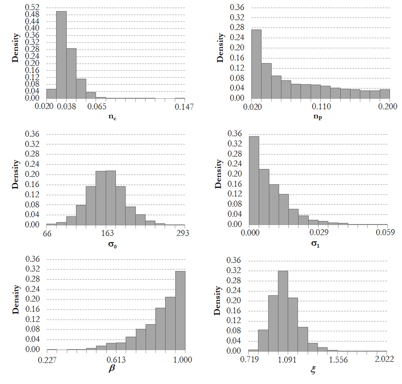
The hydraulic model parameters, $\theta$, are the Manning’s roughness coefficients for main channel (n_c) and floodplains (n_p), considered to be independent of each other, in the same cross section. For simplicity and similarly to previous studies (PAPPENBERGER et al., 2005; JUNG, 2011), it was hypothesized that two values per simulation, drawn from the prior PDFs for each of these two parameters, are sufficient to represent the roughness of the river reach considered. Pappenberger et al. (2005) showed that the performance of a hydrodynamic model is worse when considering different values of n_c and n_p between various topobathymetric cross sections, as compared to the hypothesis adopted in the present study. The preferred option also reflects the similarity of either the vegetation cover in the floodplains or the bed material in the main channel along the stream reach under study.

Further, estimates about the variability of roughness in both main channel and floodplains were made from tables shown in references such as Chow (1959), Arcement and Schneider (1989) and Hicks and Mason (1991) that would correspond to natural channels. Due to the absence of additional elements that would allow differentiation between the different possible values for this type of channel, it was defined that the prior knowledge about the uncertainty of the roughness coefficients should be described by the Uniform distribution. Inferior and superior limits were then extracted from the mentioned bibliography, and any values in this interval were assigned equiprobability.

Conceptual model for the residuals and the correspondent likelihood function

The HEC-RAS model hydrodynamic component is based on an implicit finite difference scheme for numerical solution of Saint-Venant’s equations, which involves partial differences for discharge and depth over time and space and nonlinear relationships between hydraulic and geometric variables. Due to these aspects, nonlinear behavior is expected between the input variables (inflow hydrograph at the upstream end of the reach) and the boundary and initial system conditions and the output variables, expressed in terms of hydrographs and cross-section depths of any cross section along the river reach.

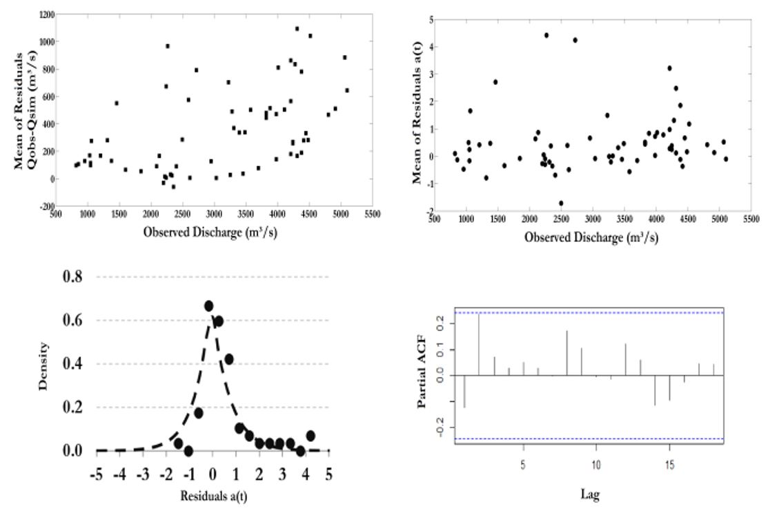
Thus, it is expected that this feature, together with the presence of several sources of uncertainties that contribute to the final uncertainty, measured through the differences $E\left(\theta \right)=\tilde{Y}-Y\left(\theta \right)$, give the latter characteristics as serial correlation, heteroscedasticity, skewness and kurtosis. To represent such assumptions mathematically, the Generalized Likelihood function proposed by Schoups and Vrugt (2010) was adopted, and thus named for its ability to synthesize a variety of statistical characteristics of the modelling residuals. To express them, these authors proposed the following statistical model for the modeling errors $e_t\left(\theta \right)$:

${\Phi }_p\left(B\right)e_t={\sigma }_t·a_t$, with $a_t~\text{SEP}\left(\mathrm{0,1,}\xi ,\beta \right)$(10)

where ${\Phi }_p\left(B\right)=1-{\displaystyle \sum }_{i=1}^p{\varphi }_i·{\text{B}}^i$ is an autoregressive polynomial with p parameters ${\varphi }_i$, $B$ is the delay operator $\left({\text{B}}^i{e}_t=e_{t-i}\right)$, ${\sigma }_t$ is the standard deviation at time t, and $a_t$ is the i.i.d. random error with zero mean and unit standard deviation, described by a distribution known as SEP (Skew Exponential Power), with parameters $\xi$ and $\beta$, which are associated, respectively, with the skewness and kurtosis expected for this type of error. The autoregressive polynomial aforementioned quantifies the serial correlation that may occur in nonlinear model residuals. Heteroscedasticity, in turn, is considered by assuming that the residuals standard deviation, ${\sigma }_t$, increases linearly with the simulated flow rate, $y_t$, i.e.:

${\sigma }_t={\sigma }_0+{\sigma }_1·y_t$ (11)

where${\sigma }_0$ and ${\sigma }_1$ are, respectively, the intercept and the slope coefficient.

Finally, the SEP distribution models the remaining noise after autocorrelation and heteroscedasticity removal, thus adapting itself to different degrees of skewness and kurtosis. Its PDF is given by the following expression (SCHOUPS; VRUGT, 2010):

$\text{p}\left(a_t|\xi ,\beta \right)=\frac{2{\sigma }_{\xi }}{\xi +{\xi }^{-1}}·{\omega }_{\beta }·\text{exp}\left(-c_{\beta }·{\left|a_{\xi ,t}\right|}^{2/\left(1+\beta \right)}\right)$ (12)

where

$a_{\xi ,t}={\xi }^{-\text{sinal}\left({\mu }_{\xi }+{\sigma }_{\xi }·a_t\right)}·\left({\mu }_{\xi }+{\sigma }_{\xi }·a_t\right)$ (13)

represent the standardized residuals $a_t$ so that parameter $\xi$ varies in the interval $\left[-\mathrm{1,1}\right]$. Additionally, ${\mu }_{\xi }$, ${\sigma }_{\xi }$, $c_{\beta }$ and ${\omega }_{\beta }$ values are calculated as functions of parameters $\xi$ and $\beta$, as in Schoups and Vrugt (2010). Special SEP cases, depending on the values assigned to these two parameters, include the Uniform, Normal, and Laplace distributions.

Considering equations 10-13, the Generalized log-likelihood function has the form of equation 14, according to the deduction described in Schoups and Vrugt (2010):

$\text{L}\left(\theta ,{\eta }_e|\tilde{Y}\right)=n·\text{log}\left(\frac{2{\sigma }_{\xi }{\omega }_{\beta }}{\xi +{\xi }^{-1}}\right)-{\displaystyle \sum }_{t=1}^n\text{log}{\sigma }_t-c_{\beta }·{\displaystyle \sum }_{t=1}^n{\left|a_{\xi ,t}\right|}^{2/\left(1+\beta \right)}$ (14)

where, similar to the notation given in Equation 7, $\theta =\left\{n_c,n_p\right\}$ is the parameter vector of the hydrodynamic model, and ${\eta }_e=\left\{{\varphi }_p,{\sigma }_0,{\sigma }_1,\xi ,\beta \right\}$ is the vector of representative variables for the residuals $e_t$, considered as latent or nuisance variables to the Bayesian inference process, and whose uncertainties will be estimated together with those corresponding to $\theta$.

It is worth noting that the error model proposed by Schoups and Vrugt (2010) also incorporates a parameter corresponding to the probable bias in outputs due to errors in input and output data, as well as in the model structure. However, it was not considered herein due to the expectation that there would not be such systematic error acting on the $Y$ vector, when compared to $\tilde{Y}$.

Numerical method for sampling the posterior PDF

For numerical estimation of the posterior joint and marginal PDFs, the MCMC method known as Differential Evolution Adaptive Metropolis, hereinafter called DREAM, and proposed by Vrugt et al. (2008a, 2008b, 2009), was used. Its algorithm has some advantages over previous MCMC techniques, such as parameter subset sampling rather than sampling from the entire parametric space, as well as outlier detection, and the use of fewer chains to ensure convergence (VRUGT, 2016). Another advantage of DREAM is its availability in Matlab software language (VRUGT et al., 2008a; 2008b; 2009; VRUGT, 2016), in the form of several subroutines that perform simulations of $N$ simultaneous Markov chains, evaluate their convergence, and also provide results such as parameter values ​​in all chains throughout the sampling process, and their posterior statistical descriptors. Some internal parameters of the method should be defined by the user, such as the number of chains, $N$, in this case in an amount equal to or greater than the total number of inferred parameters, according to Vrugt (2016); the number of iterations, denoted by T, for each chain, and of parameters (for both hydrodynamic and error models); and, finally, the likelihood function to be used. The minimum and maximum limits for each parameter, their respective prior PDFs, and the observed data vector $\tilde{Y}$, which will serve as a paradigm for the uncertainty calibration from the Bayesian perspective, must also be prescribed.

Finally, a subroutine defining the model $\mathcal{F}$ for the evaluated system must be coupled to the main DREAM routine, whose outputs will be compared with the observed data at each iteration for each Markov chain. For this purpose, a Matlab script was also prepared for command activation of the HEC-RAS Controller (GOODELL, 2014; LEON; GOODELL, 2016), a set of routines developed by USACE to automate various modeling steps in HEC-RAS, such as: data input, simulations under different flow and/or geometry scenarios and results plotting.

Parametric and predictive uncertainty estimation

To evaluate the convergence of the $N$ chains considered, the statistic of Gelman and Rubin (1992) for each parameter was calculated, as recommended by Gilks et al. (1998) and Vrugt (2016). Accordingly, the burn-in period was considered as the number of iterations $T^{*}$ required for the parameter that reached convergence last. Thus, the posterior PDF could be constructed from samples extracted from the $N·\left(T-T^{*}\right)$ iterations of each parameter throughout the $N$ chains. Since each Markov chain starts from distinct points in the multiparametric space and achieves the same stationary distribution (the target distribution, or the posterior joint PDF), the results can be estimated by merging the parameter values between the chains once convergence is reached.

From these samples, it is possible to construct histograms and to calculate point estimators and credibility intervals for each of the parameters, so as to assess the parametric uncertainty after observing the information contained in data $\tilde{Y}$.

To elaborate credibility intervals, the following concept was used, given in Equation 15 (FERNANDES; SILVA, 2017):

$\underset{L}{\overset{U}{{\displaystyle \int }}}\text{p}\left(w\right)\text{d}w=1-\alpha$ (15)

where w is the variable of interest, $\text{p}\left(w\right)$ is its probability distribution (prior, or posterior, for example), and L and U are, respectively, the lower and upper limits of the credibility range, which, in the Bayesian approach, represents the highest density probability range of containing w, at the level $100·\left(1-\alpha \right)\%$.

The construction of credibility intervals is also one of the ways to measure the predictive uncertainty for output variables extracted from the hydrodynamic model, denoted in this case by the variable $y_{\text{p}}$ and the vector $Y_p$. To do so, it is necessary to propagate the posterior uncertainties through the model, i.e. those associated either with the parameters, or with other sources, represented herein by latent variables. The $y_{\text{p}}$ percentiles, associated with a non-exceedance probability expressed by $1-\alpha$, and hereafter named as $y_{1-\alpha }$, are obtained from the following relation (SCHOUPS; VRUGT, 2010), represented in vector form:

$P\left(Y_p\le Y_{1-\alpha }|\tilde{X}\right)=\text{P}\left({\left[Y\left(\tilde{X}|\theta \right)+E\left({\eta }_e\right)\right]}_{1\cdots J}\le Y_{1-\alpha }|\tilde{X}\right)=1-\alpha$ (16)

where J sets, as formed by parameters and latent variables $\left\{\theta ,{\eta }_e\right\}$, are randomly drawn from the posterior joint FDP obtained by applying the chosen MCMC method and are used to generate J time series for model outputs, $Y$, and residuals, denoted in Equation 16 as $E\left({\eta }_e\right)$ since, in order to compose the predictive uncertainty, their generation depends on the error model parameters included in vector ${\eta }_e$. These J time series correspond to J hydrodynamic model predictions at each time interval, from which it is possible to calculate predictive percentiles $y_{1-\alpha }$ for each time step. Thus, for example, using $\text{1}-\alpha \text{= 0}\text{.975}$ and $\text{1}-\alpha \text{= 0}\text{.025}$, predictive percentiles with 97.5% and 2.5% of non-exceedance are obtained for each time step of the predicted hydrograph, which together will make up the 95% credibility interval. If $E\left({\eta }_e\right)\text{= 0}$, the predictive percentiles thus obtained embody only the predictive uncertainty associated with the parameters of the hydrodynamic model.

The computation of errors in expression (16) requires the generation of independent samples of the $\text{SEP}\left(\mathrm{0,1,}\xi ,\beta \right)$ distribution, which was performed using an algorithm provided by Schoups and Vrugt (2010) and detailed in their study. Once J series from the SEP are calculated, it is necessary to add the heteroscedasticity ${\sigma }_t$ and the serial correlation expressed by ${\varphi }_p$, with the corresponding latent variables extracted from the set $\left\{\theta ,{\eta }_e\right\}$ of each draw.

Equation 16 can be applied to the same flood used as the paradigm $\tilde{Y}$, such that to evaluate the total uncertainty contained in its simulation through the selected hydrodynamic model and calculated with the available topobathymetric information and boundary conditions. Similarly, it can also be used to estimate the predictive uncertainty of other floods, provided that the error structure in the outflow hydrographs and the parameters and latent variables uncertainty remain valid. This hypothesis seems reasonable for floods with magnitude similar to the flood used for the uncertainty calibration through the proposed scheme.

Predictive percentiles with 97.5%, 50% and 2.5% of non-exceedance corresponding to the peak discharge were used to construct the probabilistic flood inundation map at the downstream end of the river reach studied, as well as probabilistic water surface profiles along it, associated with the flood used in the Bayesian inference process. For this, the flow rates corresponding to such percentiles were simulated through the HEC-RAS model under the steady flow regime condition. In this case, as their values ​​incorporate other sources of uncertainty than that contained in the roughness coefficients, the estimated posterior median values of $n_c$ and $n_p$ were used. The results, expressed in terms of flood inundation area and depths along the stream, should be considered with caution, as further evaluations need to be performed to check whether the structure of residuals computed for these two variables is similar to that of the obtained errors corresponding to outflow hydrographs.

Characterization of the river reach and data availability

The methodology was applied to a reach of the Upper São Francisco river, between the Abaeté river mouth and the city of Pirapora, in the state of Minas Gerais, within UTM SIRGAS 2000 (zone 23S) coordinates of 473,600 and 513,700 E and 8,005,150 and 8,087,000 N, making up about 100-km length, as shown in Figure 1.

Figure 1
Studied river reach position in relation to the regional drainage network.

This reach has 2 upstream river gauges, operated by CEMIG - Companhia Energética de Minas Gerais, one located on the São Francisco river and the other on the Abaeté river, 30 km and 40 km upstream of their confluence, respectively. At the downstream end, next to the BR-365 highway bridge, in the urban area of Pirapora, there is another river gauge, operated by the Brazilian Geological Survey (CPRM), whose daily mean flow records were considered as the $\tilde{Y}$ information, particularly those related to the major floods on the record. The position of the stream gauges in relation to the river network of interest is shown in Figure 1 and some of their features are summarized in Table 1.

Table 1
Characteristics of the stream gauges used.

Code ( ANA, 2009 )	Name	Operator	River name	Geographical Coordinates SIRGAS2000		Data Availability	Drainage Area (km2)
				Latitude	Longitude
41020002	UHE Três Marias Jusante	CEMIG	São Francisco river	18°11'13”O	45°15'10”S	01/1957 to 11/2017	50,816
41090002	PCH Salto do Paraopeba Ponte BR 040	CEMIG	Abaeté river	18°06'32”O	45°27'43”S	04/1963 to 11/2017	5,186
41135000	Pirapora Barreiro	CPRM	São Francisco river	17º22'09”O	44º56'36”S	06/1968 to 11/2016	62,200

Due to the existence of the Três Marias hydropower plant upstream, CEMIG has carried out topobathymetric surveys on several occasions, which make up the extension from the dam to the city of Pedras de Maria da Cruz, about 300 km downstream. For the reach selected in this study, there are 22 cross sections available, surveyed in 2011, whose locations are indicated in Figure 1.

Also available is an MDT constructed by CEMIG for the riverbed and floodplains along the reach between the Abaeté river mouth and the city of Pirapora, with 1m x 1 m horizontal resolution, which encompasses the banks and a 1 to 2 km wide band in the floodplains from each bank.

Hydraulic model construction and its coupling to DREAM

With this information, it was possible to develop a preliminary 1D hydraulic model in the preselected reach, which was extended to the mouth of the Velhas river, in order to verify the dominant flow regime, the presence and influence of hydraulic controls and their representation by the available cross sections, and, finally, to decide on the actual reach features that needed to be represented by the model. This appraisal was conducted mainly due to the expectation that the flow regime would be predominantly subcritical, which requires the prescription of a downstream control condition. Although the rating curve of the downstream river gauge (Pirapora-Barreiro; code 41135000) could be an excellent boundary condition in other circumstances, it was not applied in the present case, since the aim was precisely to evaluate the errors between the observed flows in the corresponding cross section and those simulated by the model. Thus, the river reach finally selected was that from the Abaeté river mouth to the cross section that acts as the hydraulic control for the downstream river gauge.

In view of the information expressed in the available topobathymetric cross sections, it was verified that the rapids located in the upstream part of the river stream along the city of Pirapora operate as a control for discharges up to 5,000 m³/s at Pirapora-Barreiro gauge. Above this threshold, the backwater effect caused by the confluence between the São Francisco and the Velhas rivers needs to be taken into account, and additional sources of uncertainty should be considered in the inference process in order to represent the hydraulic control and the effects imposed by this important tributary. Thus, since the main objective is to verify the applicability of the methodology in order to quantify the parameter uncertainties and the total predictive uncertainty, it was defined that the model should finish at the cross section located immediately upstream to these rapids, considering flood propagation up to the abovementioned threshold flow.

To estimate these uncertainties, respecting the indicated upper flow limit conditioned by critical downstream control, the February 1992 flood event, one of the largest recorded in the Upper São Francisco river, was selected. The peak discharge at the downstream gauge, Pirapora-Barreiro, has reached 5,098 m³/s. The hydrograph considered as an upstream boundary condition was obtained by summing the daily mean discharges at the two upstream gauges, under the assumption that the propagation effect would not be significant due to the short reach length from these gauges until the confluence between the Abaeté and São Francisco rivers. Thus, the inflow peak discharge was estimated to be 4,577 m³/s. In addition, lateral inflows were not considered, due to the lack of river gauges on main tributaries and to the fact that the incremental area is not higher than 10%. In this case, it was assumed that the uncertainties entailed by flood hydrograph estimates in ungauged basins obtained from rainfall-runoff modeling or by regionalization methods would be greater than the difference between the downstream river gauge drainage area and the sum of the contributions to the two upstream gauges.

The data selected as the$\tilde{Y}$ vector for updating the prior information span the period from 12/01/1992 to 16/03/1992, and was selected to ensure the stability of the hydraulic model and to fully represent the rising and falling limbs of the flood hydrograph. After a series of simulations in steady and unsteady regimes to assess the sensitivity to the boundary conditions, the flow range and the predefined limits for the roughness coefficients, the hydraulic model, as constructed in the light of the mentioned information and assumptions, was coupled to the DREAM method toolbox. To this end, a Matlab routine was designed to open the HEC-RAS application at each iteration of the Markov chains in order to access the constructed model and change the parameters under evaluation, in this case, the Manning’s roughness coefficients.

Table 2 summarizes the prior distributions and their respective limits considered for the hydraulic model parameters, $\theta =\left\{n_c,n_p\right\}$, and the error model parameters, ${\eta }_e=\left\{{\varphi }_p,{\sigma }_0,{\sigma }_1,\xi ,\beta \right\}$, as well as their units.

Table 2
Prior distributions and lower and upper limits assigned to the parameters of the vectors $\theta$and ${\eta }_e$.

Name	Notation	Unit	Prior PDF	Inferior bound	Superior bound
Manning's roughness coefficient in the main channel	nc	-	UNIFORM	0.012	0.150
Manning's roughness coefficient in the floodplains	np	-		0.020	0.200
Standard deviation: intercept	σ0	m3/s		0	1000
Standard deviation: slope coefficient	σ1	−		0	1
Kurtosis	β	−		-1	1
Skewness	ξ	−		0.1	10
p-order serial correlation coefficient	ϕp	-		0	1

RESULTS

In the MCMC numerical scheme, 8 Markov chains were used, each with 8,000 iterations, so that each parameter of the vector $\left\{\theta ,{\eta }_e\right\}$ could have a maximum of 64,000 iterations. Of these, the first 14,000 (i.e. 1,750 per chain) were discarded as a burn-in period, considering the number of iterations required for the last parameter to reach convergence according to the Gelman-Rubin criterion.

Observing the autocorrelation values for each parameter along each chain, it was decided to skip 5 lags in order to compose the final samples, so that to ensure an adequate sampling of each chain, with the attributes of being representative and long enough for the 7 parameters to be inferred, following recommendations by Vrugt (2016). Thus, the results were obtained on the basis of $\left[N·\left(T-T^{*}\right)\right]/\text{lag}$= 10,000 samples extracted from the 8 chains, for each parameter.

The initial criterion for MCMC simulations was the need for 5 latent variables to adequately represent the modeling residuals, namely: ${\varphi }_1$, assuming that an AR (1) model would be sufficient to explain their serial correlation; ${\sigma }_0$ and ${\sigma }_1$, expecting a linear increase in variance with simulated discharge; and $\beta$ and $\xi$, to model, respectively, kurtosis and the existence of heavy tails, and skewness that may occur in the error series after the removal of autocorrelation and heteroscedasticity. The linear model for the variance as a function of the discharge magnitude expresses the hypothesis that flows extracted from the upper branch of rating curves might have greater relative errors than those corresponding to discharges in the middle and lower branches, as mentioned by Potter and Walker (1985), Kuczera (1996), and Domeneghetti et al. (2012).

The results under this criterion (not shown in here) indicated that although the modeling residuals $e_t\left(\theta \right)$ met their assumptions, the posterior estimates for the parameters of the hydrodynamic and error models yielded very large 95% uncertainty bands for the outflow hydrograph, including negative 2.5% percentiles in the descending limb. This unfavorable aspect was credited to the high values inferred to ${\varphi }_1$, with a mean value of 0.9. Values close to the unit produce time series that are similar to a random walk, resulting in large random errors. Such behavior was found in the uncertainty calibration of a hydrological model through a Bayesian scheme in one of the watersheds studied by Schoups and Vrugt (2010).

For this reason, new tests were performed, considering an AR (2) model. Although in this scenario the mean of ${\varphi }_1$ has decreased in comparison to its value in the previous case, accounting for serial correlation up to lag 2 still yielded very large values for the 95% uncertainty range, with negative discharges at the lower limit of the hydrograph falling limb.

Additionally, the values of the 1^st order autocorrelation coefficients for the $E\left(\theta \right)$ residual series generated from the prior PDFs of the vector $\theta$ were estimated. A mean value of 0.75 was obtained, which is quite different from the value of 0.90 estimated in the first scenario. However, the still high value is thought to be due to the influence of the rising branch of the inflow hydrograph, which is quite pronounced as compared to its middle portion and its descending branch. This aspect might have been intensified by not accounting the lateral inflows into the hydrodynamic simulations.

From these first results, and given the relevance of parameter ${\varphi }_1$ in composing the predictive uncertainty in the present situation, a new scenario was defined, in which ${\eta }_e=\left\{{\varphi }_1,{\sigma }_0,\xi ,\beta \right\}$. In this case, parameter ${\sigma }_1$ was set to a constant value, estimated from other previously tested scenarios, in which invariably its mean tended to 0.01. Again, the posterior distribution for ${\varphi }_1$showed an aspect similar to that produced in the first scenario, with a mean close to 0.90.

Given the overestimation of ${\varphi }_1$ in the scenarios previously simulated, and in order to obtain more realistic intervals for the total predictive uncertainty, this variable was removed from the Bayesian uncertainty calibration, by fixing its value in a procedure similar to that described by Schoups and Vrugt (2010) and Silva et al. (2014). To this end, it was defined that ${\varphi }_1$ = 0.75, obtained directly from the $E\left(\theta \right)$ series, as outlined above. Thus, the inference process followed with the presence of 5 latent variables, being ${\varphi }_1$ constant, and ${\sigma }_0$, ${\sigma }_1$, $\beta$ and$\xi$ subject to the estimation of their uncertainties, with uniform prior PDFs, defined within the lower and upper bounds shown in Table 2.

In order to corroborate the hypotheses established for the residuals $e_t\left(\theta \right)$, several evaluations of these and of the residuals after removing serial correlation were made, followed by heteroscedasticity extraction. The residuals thus obtained, denoted by $a_t$ (see Equation 10), in theory should follow a SEP distribution with zero mean, unit standard deviation, parameter $\beta$ between -1 and 1, and $\xi \text{> 0}$. Part of these analyses is illustrated in Figure 2.

Figure 2
Behavior of the hydrodynamic modeling residuals under the hypotheses of serial correlation, heteroscedasticity, skewness and kurtosis.

It is observed that the residuals $e_t\left(\theta \right)$actually have variance that depends on the observed flow magnitude $\tilde{Y}$ (graph 02.a), although it undoubtedly becomes stable from a given discharge value on (about $\tilde{Y}$ > 2,000 m³/s). After the heteroscedasticity removal (graph 02.b), the dispersion in relation to $\tilde{Y}$ presents constant aspect, except for some points that remained more scattered. The mean values ​​of residuals $a_t$, obtained at each time step $t$ of the outflow hydrograph, in turn, show adherence to part of the SEP distribution (0,1,$\widehat{\beta }$, $\widehat{\xi }$), with $\widehat{\beta }$ and $\widehat{\xi }$ drawn from the set ${\eta }_e=\left\{{\sigma }_0,{\sigma }_1,\xi ,\beta \right\}$ which presented the highest value for log-likelihood $\text{L}\left(\theta ,{\eta }_e|\tilde{Y}\right)$, equal to 0.978 and 1.078, respectively (graph 02.c: probability density of empirical quantiles versus theoretical ones - markers versus dotted line). These values ​​indicate that residuals after serial correlation and heteroscedasticity removal adhere to an approximately symmetrical Laplace distribution, with a sharper pattern than a Normal distribution. This shows that the stipulated error model is more representative of outliers than a model under the normality hypothesis, as argued by Schoups and Vrugt (2010). It is worth to note, however, that the series formed by the empirical quantiles, as corresponding to the mean values ​​of the residuals $a_t$, has positive skewness, with higher concentration of points to the right side of its mean (whose value is close to 0.00), as shown in graph 02.c. Part of the posterior values of$\widehat{\xi }$ (between about 1.00 and 1.367 – see Table 3) reflects this behavior, as values of $\widehat{\xi }$ greater than 1.0 denote positive skewness in the $\text{SEP}\left(\mathrm{0,1,}\xi ,\beta \right)$ distribution. It is estimated that the skewness of the $a_t$series could be better represented by the parameter$\widehat{\xi }$ if more points (i.e. observed flows) were used as information $\tilde{Y}$ in order to feed the DREAM numerical scheme. Using the sgedFit routine from the fGarch package (WUERTZ et al., 2017) in the R Studio computer program, it was possible to estimate the parameter $\widehat{\xi }$ of all $a_t$ series calculated after removing serial correlation with ${\varphi }_1$= 0.75 and the corresponding values of ${\sigma }_t$ from the $E\left(\theta \right)$ series obtained with the posterior $\theta$ samples. There was a dispersion of $\widehat{\xi }$ around 0.9 and 2.1 (interquartile amplitude), so that the posterior PDF calibrated for this parameter, centered around 1.054 and with 97.5% percentile equal to 1.367, partly represents the actual skewness values ​​of the $a_t$ series.

Table 3
Posterior statistical descriptors of the hydrodynamic model parameters and the generalized log-likelihood parameters.

Parameter	Mean	Standard deviation	Mode	Median	Skewness Coefficient	2.5% Percentile	97.5% Percentile
nc	0.039	0.009	0.030	0.037	1.913	0.027	0.061
np	0.076	0.052	0.026	0.058	0.792	0.021	0.190
σ0	164	30.2	225	164	0.173	107	227
σ1	0.009	0.008	0.000	0.007	1.636	0.000	0.030
β	0.865	0.118	0.935	0.896	-1.189	0.562	0.996
ξ	1.064	0.133	0.955	1.054	1.149	0.855	1.367

Finally, the partial correlogram constructed for the mean values ​​of $a_t$ (graph 02.d) indicates that the use of coefficient ${\varphi }_1$ equal to 0.75 guarantees the elimination of serial correlation with respect to the previous time step.

Since the residuals met most of the hypotheses that compose the error model, and the generalized log-likelihood function was adequate to explain them, it was possible to carry out the posterior parametric uncertainty inference. Figure 3 shows the histograms of the hydrodynamic model parameters and latent variables based on 10,000 samples for each one.

Figure 3
Posterior distributions of the hydrodynamic model parameters and the generalized likelihood parameters.

The graphs show that, in most cases, there was a significant reduction of the prior uncertainty stipulated, so that the $\tilde{Y}$ data used added information to the previously estimated uncertainties of a 1D hydrodynamic model using a Bayesian scheme, under the assumption of a likelihood function appropriate to the residuals. Some statistical descriptors of the parameters of the vectors $\theta$ and ${\eta }_e$ are summarized in Table 3.

The posterior mean value for the Manning’s coefficient in the main channel was 0.039, with a standard deviation of 0.009, indicating a more accurate identification when compared to that presented by the roughness in the floodplains. In this case, the standard deviation was 0.052, 6 times higher than in the main channel, with a posterior mean of 0.076.

The posterior mode, in turn, was 0.026, close to the lower bound initially established for this parameter. Inspection of log-likelihood values ​​(results not shown here) reveals that their global maximum occurs at $n_p$ = 0.032, with local maxima encountered for the entire prior range. Based on these results, it is hypothesized that the flood used was not of sufficient magnitude to cause floodplain inundation to the extent of better identifying the roughness in this region. In fact, the return period for the 1992 event is around 10 years. There are records of larger floods, such as in 1979, but their use would add complexity to the boundary conditions considered in the model and could eventually result in additional uncertainties.

Similarly to $n_c$, latent variables also had their limits significantly narrowed as compared to the prior condition. It is indeed noticeable that parameter ${\sigma }_1$, with a mean close to 0, cannot be disregarded since its posterior values, when multiplied by the downstream discharges and summed to ${\sigma }_0$, provide mean standard deviations between 140 and 270 m³/s, for the highest flow rates of the observed hydrograph, and between 120 m³/s and 230 m³/s for the lowest flows. Some tests were performed considering the variance constant over time, and it was observed that the ${\sigma }_0$ posterior PDF compensates for the absence of ${\sigma }_1$. In addition, evaluations conducted for residuals provide evidence that the hypothesis of heteroscedasticity seems more correct in the present case, although the results indicate the need for a longer flood event to better identify ${\sigma }_t$. Furthermore, graph 02.b, where the variance becomes constant after heteroscedasticity removal, with the exception of a few points, may indicate that different variance models, other than linear, should be tested for the hydrodynamic modeling. In such a case, larger modeling errors can occur for discharges that cause small water depths in the floodplain, just after the overflow of river banks, for example.

$\widehat{\beta }$, in turn, corroborates the adherence of the residuals $a_t$ to a Laplace distribution, with its mean tending to unity, according to the SEP standardization shown in Schoups and Vrugt (2010). Finally, the posterior PDF of $\xi$ represented, in part, the actual skewness of the i.i.d. residuals. Obviously, other distributive models for residuals after removal of serial dependence and heteroscedasticity can be adjusted as long as they adapt to the existing kurtosis and skewness in the posterior series obtained.

The dependence relationship between hydrodynamic model parameters and latent variables subject to Bayesian inference can be seen in the scatter plots in Figure 4.

Figure 4
Scatter plots for posterior values of the hydrodynamic model parameters and latent variables.

It is observed that $n_c$ values ​​greater than 0.050 necessarily correspond to smaller $n_p$ values ​​(below 0.100), although these also occur for the entire posterior amplitude of the main channel roughness. This may explain the posterior linear correlation coefficient equal to -0.50 between these two parameters. In turn, ${\sigma }_0$ and ${\sigma }_1$ show a clear negative linear correlation (with a coefficient of -0.55, the largest of all), which might be expected due to the prescription of the error model (Equation 11) and to the values ​​of ${\sigma }_t$ compared to the discharge magnitude at $\tilde{Y}$. In other combinations between parameters of $\theta$ and ${\eta }_e$, there is no important linear dependence, so that the respective linear correlation coefficients vary between -0.41 and 0.14. Schoups and Vrugt (2010) point out values ​​for this coefficient whose modulus should be equal to or greater than 0.70 as an indicator of possible overestimation of the number of parameters subject to calibration, with the possibility of setting as constant the values of some of them.

Subsequently, sets of parameters and latent variables were drawn from the 10,000 posterior joint samples for the predictive uncertainty composition associated with the 1992 flood and events similar in magnitude. Regarding the prediction of the outflow hydrograph at the downstream end of the river reach, measured at Pirapora-Barreiro river gauge (Figure 5), it is verified the 95% credibility interval amplitude attains between 730 m³/s (at the beginning of the hydrograph, with observed discharges around 1,000 m³/s) and 2,500 m³/s (near the peak flow, around 5,100 m³/s), considering all sources of uncertainty. In absolute terms, larger uncertainties (amplitudes) occur along with the highest flow rates observed, as well as in the 2^nd half of the rising limb of the hydrograph. However, in relative terms (amplitude/observed flow), the largest uncertainties occur in the descending part of the hydrograph, due to the persistence of a high amplitude and to the discharge reduction. These results may have arisen from the use of an autoregressive model for the residuals $e_t\left(\theta \right)$ and from using Equation 10 to obtain $E\left({\eta }_e\right)$, with a high value for the coefficient ${\varphi }_1$, so that the residuals in the falling limb present high values, with magnitude similar to those near the peak flow. Heteroscedasticity has indeed less influence than ${\varphi }_1$ on error composition in the present study. Moreover, even though the value of this parameter has been set at 0.75, the last 6 discharge values at the lower limit of the 95% credibility interval, corresponding to 2.5% percentiles, are negative, reaching -341 m³/s. However, lower values ​​for ${\varphi }_1$ would certainly lead to partial removal of the 1^st order serial correlation between the residuals, interfering with the posterior uncertainty estimation of the other latent variables and the roughness coefficients. One possible way to overcome this limitation of the method with effects on the composition of predictive uncertainty consists in applying the autoregressive model to the standardized residuals obtained after serial correlation removal, instead of doing so to the raw heteroscedastic residuals, as proposed by Evin et al. (2013).

Figure 5
Credibility intervals at a level of 95% for the 1992 flood outflow hydrograph in the studied fluvial reach, representing the total predictive uncertainty.

In addition, it is observed that the posterior parametric uncertainty has a much smaller effect on total predictive uncertainty compared to other sources of uncertainty, expressed by the vector ${\eta }_e$. In this case, the amplitude over the total uncertainty credibility interval varies around 10.0 m³/s and 370 m³/s, with higher absolute values ​​corresponding to the regions of the observed hydrograph with greater slope, either on the rise, or in the recession. It is also noted the difficulty of the model to reproduce the observed flow rates in the hydrograph rising limb, even varying the Manning’s coefficients within their respective posterior ranges. On the contrary, the flood recession is reproduced properly, with observed discharges within the parametric predictive uncertainty range for the most part of it. This phenomenon probably has occurred due to the absence of lateral inflows from ungauged tributaries, which may have been important in shaping the 1992 flood hydrograph at Pirapora-Barreiro cross section. In fact, this was a flood caused by widespread and long-duration rainfall on the Upper São Francisco river basin. Incremental basins, of significantly smaller magnitude than that of the upstream basin, and without the propagation effect induced by the Três Marias reservoir, may have contributed to significant volumes and peaks in the flood hydrograph rise, particularly from the dam releases, causing the difference between observed and simulated discharges. This is also likely to be the cause of the high values ​​of ${\varphi }_1$ calculated for the $E\left(\theta \right)$ series. It is expected that the accounting of the lateral flows into the modeling would certainly reduce the values of ${\varphi }_1$, thus leading to smaller total predictive uncertainty bands.

Future tests, complementary to this work, should evaluate the impact of the insertion of such inflows on the uncertainty calibration by means of a Bayesian scheme, in particular on the modeling residuals behavior. This is expected to reduce the final predictive uncertainty associated with the 1992 flood.

Figures 6 and 7 depict, respectively, the probabilistic water surface profiles, and the probabilistic flood inundation area in the face of total predictive uncertainty, in both cases corresponding to the peak discharge in the downstream river gauge. In the second case, emphasis was given to the urban region of Pirapora that borders the focused river reach. The portion downstream the rapids has not been studied because it has relevant interference from the backwater effect caused by the Velhas river.

Figure 6
Credibility intervals at a level of 95% for the water surface profiles along the studied fluvial reach, considering the total predictive uncertainty.

Figure 7
1992 flood probabilistic inundation map in the upstream portion of Pirapora.

It can be seen from Figure 7, as a result of the shape of the river valley in the mapped area and of the wide variation of peak discharges induced by the wide credibility interval, that the flood inundation extent varies significantly between the lower and upper discharge limits, under the adoption of median values ​​for the Manning’s roughness coefficients in the main channel and the floodplains. It is worth remembering that these results are approximate, as they rely on the hypothesis of steady flow regime, on the one hand, and on the statistical structure of the residuals associated with the outflow hydrograph, on the other. Further complementary simulations should be performed in order to investigate the impact of using other variables as $\tilde{Y}$ paradigms on parametric uncertainties calibration, as well as those arisen from other sources of modeling errors.

Another aspect shown in Figure 7 refers to the small difference between the inundation area reached by the peak discharges 50% and 97.5% percentiles that make up the 95% credibility range. This may be due in part to the river valley morphology and to the stage-discharge relationship in its upper branch in the downstream end of the reach. Added to this there is a certain limitation of the available topobathymetric survey and the MDT used, whose information was not sufficient to depict the entire floodplain at some sections.

CONCLUSIONS AND RECOMMENDATIONS

This study showed how it is possible to estimate the uncertainties associated with hydrodynamic modeling through a Bayesian scheme in which prior knowledge about roughness variability is updated with observed information from some descriptive variable of the phenomenon in question, in this case, the flow rates gauged at the downstream end of the studied river reach, located in the upper São Francisco river.

It is recommended to verify the methodology for a flood with similar magnitude to the one used for the uncertainty calibration process by sampling roughness coefficients from their posterior PDFs and performing thousands of simulations to construct the credibility intervals for the outflow hydrograph. To obtain the total predictive uncertainty, synthetic residuals should be added modeled by the error distribution considered.

The applied methodology shows the relevance of systematic monitoring of variables such as stage, discharge, and even velocities, with potential use for calibration of hydrodynamic model parameters, either from their point estimators or their uncertainties.

Even two-dimensional models, powered by more accurate digital terrain models, can have their uncertainties considerably increased if there is not enough data to calibrate them.

Another aspect emanating from the results refers to the relevance of considering lateral inflows to the hydrodynamic simulations in the present case, although these flows need to be estimated by indirect methods, such as regionalization or spatial transfer of hydrometric information.

Future checks on the sensitivity of the parameter uncertainties of both the hydrodynamic model and the error model to the observed variable used in the calibration process, as well as the amount of observed data, n, are also provided in the context of the continuity of the research reported in this paper.

ACKNOWLEDGEMENTS

The authors thank the Brazilian Geological Survey (CPRM), and CEMIG - Companhia Energética de Minas Gerais, for providing the data used, to FAPEMIG, for the PhD scholarship to the first author, and to CNPq for the research productivity scholarship to the second author. Finally, the authors would like to thank the anonymous reviewer for their valuable comments and suggestions.

REFERENCES

• ALI, A. M.; SOLOMATINE, D. P.; DI BALDASSARE, G. Assessing the impact of different sources of topographic data on 1-D hydraulic modelling of floods. Hydrology and Earth System Sciences, v. 19, n. 1, p. 631-643, 2015. http://dx.doi.org/10.5194/hess-19-631-2015
  » http://dx.doi.org/10.5194/hess-19-631-2015
• ANA – AGÊNCIA NACIONAL DE ÁGUAS. Inventário das Estações Fluviométricas 2nd ed. Brasília: ANA, 2009.
• ARCEMENT, G. J.; SCHNEIDER, V. R. Guide for selecting manning’s roughness coefficients for natural channels and flood plains: Water supply - Paper 2339 Los Angeles: U. S. Geological Survey, 1989.
• AYYUB, B. M.; KLIR, G. J. Uncertainty modeling and analysis in engineering and the sciences Boca Raton: Chapman and Hall/CRC, 2006.
• BEVEN, K. A manifesto for the equifinality thesis. Journal of hydrology, v. 320, n. 1-2, p. 18-36, 2006.
• BEVEN, K.; BINLEY, A. GLUE: 20 years on. Hydrological Processes, v. 28, n. 24, p. 5897-5918, 2014.
• BEVEN, K.; BINLEY, A. The future of distributed models: model calibration and uncertainty prediction. Hydrological Processes, v. 6, n. 3, p. 279-298, 1992.
• BEVEN, K.; LEEDAL, D.; MCCARTHY, S. Framework for assessing uncertainty in fluvial flood risk mapping London: FRMRC, 2011.
• BLASONE, R.-S.; VRUGT, J. A.; MADSEN, H.; ROSBJERG, D.; ROBINSON, B. A.; ZYVOLOSKI, G. A. Generalized likelihood uncertainty estimation (GLUE) using adaptive Markov Chain Monte Carlo sampling. Advances in Water Resources, v. 31, n. 4, p. 630-648, 2008. http://dx.doi.org/10.1016/j.advwatres.2007.12.003
  » http://dx.doi.org/10.1016/j.advwatres.2007.12.003
• BOZZI, S.; PASSONI, G.; BERNARDARA, P.; GOUTAL, N.; ARNAUD, A. Roughness and discharge uncertainty in 1D water level calculations. Environmental Modeling and Assessment, v. 20, n. 4, p. 343-353, 2015. http://dx.doi.org/10.1007/s10666-014-9430-6
  » http://dx.doi.org/10.1007/s10666-014-9430-6
• CAMACHO, R. A.; MARTIN, J. L.; MCANALLY, W.; DÍAZ‐RAMIREZ, J.; RODRIGUEZ, H.; SUCSY, P.; ZHANG, S. A comparison of Bayesian methods for uncertainty analysis in hydraulic and hydrodynamic modeling. Journal of the American Water Resources Association, v. 51, n. 5, p. 1372-1393, 2015. http://dx.doi.org/10.1111/1752-1688.12319
  » http://dx.doi.org/10.1111/1752-1688.12319
• CHENG, Q. B.; CHEN, X.; XU, C. Y.; REINHARDT-IMJELA, C.; SCHULTE, A. Improvement and comparison of likelihood functions for model calibration and parameter uncertainty analysis within a Markov chain Monte Carlo scheme. Journal of Hydrology (Amsterdam), v. 519, p. 2202-2214, 2014. http://dx.doi.org/10.1016/j.jhydrol.2014.10.008
  » http://dx.doi.org/10.1016/j.jhydrol.2014.10.008
• CHOW, V. T. Open-channel hydraulics New York: McGraw-Hill, 1959. vol. 1.
• COOK, A.; MERWADE, V. Effect of topographic data, geometric configuration and modeling approach on flood inundation mapping. Journal of Hydrology, v. 377, n. 1, p. 131-142, 2009. http://dx.doi.org/10.1016/j.jhydrol.2009.08.015
  » http://dx.doi.org/10.1016/j.jhydrol.2009.08.015
• DI BALDASSARRE, G.; SCHUMANN, G.; BATES, P.D.; FREER, J.E.; BEVEN, K.J. Flood-plain mapping: a critical discussion of deterministic and probabilistic approaches. Hydrological Sciences Journal – Journal des Sciences Hydrologiques, v. 55, n. 3, p. 364-376, 2010.
• DOMENEGHETTI, A.; CASTELLARIN, A.; BRATH, A. Assessing rating-curve uncertainty and its effects on hydraulic model calibration. Hydrology and Earth System Sciences, v. 16, n. 4, p. 1191-1202, 2012. http://dx.doi.org/10.5194/hess-16-1191-2012
  » http://dx.doi.org/10.5194/hess-16-1191-2012
• EVIN, G.; KAVETSKI, D.; THYER, M.; KUCZERA, G. Pitfalls and improvements in the joint inference of heteroscedasticity and autocorrelation in hydrological model calibration. Water Resources Research, v. 49, n. 7, p. 4518-4524, 2013. http://dx.doi.org/10.1002/wrcr.20284
  » http://dx.doi.org/10.1002/wrcr.20284
• FERNANDES, W.; SILVA, A. T. Introduction to bayesian analysis of hydrologic variables. In: NAGHETTINI, M. Fundamentals of statistical hydrology New York: Springer, 2017. Chap. 11, p. 497-536. http://dx.doi.org/10.1007/978-3-319-43561-9_11
  » http://dx.doi.org/10.1007/978-3-319-43561-9_11
• GELMAN, A.; RUBIN, D. B. Inference from iterative simulation using multiple sequences. Statistical science, v. 7, n. 4, p. 457-472, 1992.
• GILKS, W. R.; RICHARDSON, S.; SPIEGELHALTER, D. Markov chain Monte Carlo in practice Boca Raton: CRC press, 1998.
• GOODELL, C. Breaking the HEC-RAS Code: A user’s guide to automating HEC-RAS Portland: H2ls, 2014.
• HALL, J. W. Handling uncertainty in the hydroinformatic process. Journal of Hydroinformatics, v. 5, n. 4, p. 215-232, 2003. http://dx.doi.org/10.2166/hydro.2003.0019
  » http://dx.doi.org/10.2166/hydro.2003.0019
• HASTINGS, W. Monte Carlo sampling methods using Markov chains and their application. Biometrika, v. 57, n. 1, p. 97-109, 1970. http://dx.doi.org/10.1093/biomet/57.1.97
  » http://dx.doi.org/10.1093/biomet/57.1.97
• HICKS, D. M.; MASON, P. D. Roughness characteristics of New Zealand Rivers: A handbook for assigning hydraulic roughness coefficients to river reaches by the” visual comparison” approach. Wellington: Water Resources Survey, 1991.
• HUTTON, C. J.; VAMVAKERIDOU-LYROUDIA, L. S.; KAPELAN, Z.; SAVIC, D. A. Uncertainty quantification and reduction in Urban Water Systems (UWS) Modelling: evaluation report. European Commission, 2011.
• JUNG, Y. Uncertainty in flood inundation mapping 2011. 143 f. Thesis (Doctorate of Philosophy – Ph.D., Civil Engineering) - Purdue University, West Lafayette, Indiana, 2011.
• JUNG, Y.; MERWADE, V. Estimation of uncertainty propagation in flood inundation mapping using a 1-D hydraulic model. Hydrological Processes, v. 29, n. 4, p. 624-640, 2015. http://dx.doi.org/10.1002/hyp.10185
  » http://dx.doi.org/10.1002/hyp.10185
• JUNG, Y.; MERWADE, V. Uncertainty quantification in flood inundation mapping using generalized likelihood uncertainty estimate and sensitivity analysis. Journal of Hydrologic Engineering, v. 17, n. 4, p. 507-520, 2012. http://dx.doi.org/10.1061/(ASCE)HE.1943-5584.0000476
  » http://dx.doi.org/10.1061/(ASCE)HE.1943-5584.0000476
• KAVETSKI, D.; FRANKS, S. W.; KUCZERA, G. Confronting input uncertainty in environmental modelling. In: DUAN, Q.; GUPTA, H. V.; SOROOSHIAN, S.; ROUSSEAU, A. N.; TURCOTTE, R. Calibration of watershed models Washington: American Geophysical Union, 2003. v. 6, Chap. 4, p. 49-68. http://dx.doi.org/10.1029/WS006p0049
  » http://dx.doi.org/10.1029/WS006p0049
• KAVETSKI, D.; KUCZERA, G.; FRANKS, S. W. Bayesian analysis of input uncertainty in hydrological modeling: 1. Theory. Water Resources Research, v. 42, n. 3, p. 1-9, 2006. http://dx.doi.org/10.1029/2005WR004368
  » http://dx.doi.org/10.1029/2005WR004368
• KUCZERA, G. Correlated rating curve error in flood frequency inference. Water Resources Research, v. 32, n. 7, p. 2119-2127, 1996. http://dx.doi.org/10.1029/96WR00804
  » http://dx.doi.org/10.1029/96WR00804
• LEON, A. S.; GOODELL, C. Controlling HEC-RAS using MATLAB. Environmental Modelling & Software, v. 84, p. 339-348, 2016. http://dx.doi.org/10.1016/j.envsoft.2016.06.026
  » http://dx.doi.org/10.1016/j.envsoft.2016.06.026
• MERWADE, V.; OLIVERA, F.; ARABI, M.; EDLEMAN, S. Uncertainty in flood inundation mapping current issues and future directions. Journal of Hydrologic Engineering, v. 13, n. 7, p. 608-620, 2008. http://dx.doi.org/10.1061/(ASCE)1084-0699(2008)13:7(608)
  » http://dx.doi.org/10.1061/(ASCE)1084-0699(2008)13:7(608)
• METROPOLIS, N.; ROSENBLUTH, A.; ROSENBLUTH, M.; TELLER, A.; TELLER, E. Equation of state calculations by fast computing machines. The Journal of Chemical Physics, v. 21, n. 6, p. 1087-1092, 1953. http://dx.doi.org/10.1063/1.1699114
  » http://dx.doi.org/10.1063/1.1699114
• MILOGRANA, J. Sistemática de auxílio à decisão para a seleção de alternativas de controle de inundações urbanas 2009. 316 f. Thesis (Doctorate in Environmental Technology and Water Resources) - Departamento de Engenharia Civil e Ambiental, Universidade de Brasília, Brasília, 2009.
• MISHRA, S. K.; SINGH, V. Soil Conservation Service Curve Number (SCS-CN) Methodology Dordrecht: Springer, 2003. http://dx.doi.org/10.1007/978-94-017-0147-1
  » http://dx.doi.org/10.1007/978-94-017-0147-1
• PAPPENBERGER, F.; BEVEN, K.; HORRITT, M.; BLAZKOVA, S. Uncertainty in the calibration of effective roughness parameters in HEC-RAS using inundation and downstream level observations. Journal of Hydrology, v. 302, n. 1, p. 46-69, 2005. http://dx.doi.org/10.1016/j.jhydrol.2004.06.036
  » http://dx.doi.org/10.1016/j.jhydrol.2004.06.036
• PAPPENBERGER, F.; MATGEN, P.; BEVEN, K. J.; HENRY, J. B.; PFISTER, L.; FRAIPONT, P. Influence of uncertain boundary conditions and model structure on flood inundation predictions. Advances in Water Resources, v. 29, n. 10, p. 1430-1449, 2006. http://dx.doi.org/10.1016/j.advwatres.2005.11.012
  » http://dx.doi.org/10.1016/j.advwatres.2005.11.012
• POTTER, K. W.; WALKER, J. F. An empirical study of flood measurement error. Water Resources Research, v. 21, n. 3, p. 403-406, 1985. http://dx.doi.org/10.1029/WR021i003p00403
  » http://dx.doi.org/10.1029/WR021i003p00403
• SCHARNAGL, B.; IDEN, S. C.; DURNER, W.; VEREECKEN, H.; HERBST, M. Inverse modelling of in situ soil water dynamics: Accounting for heteroscedastic, autocorrelated, and non-Gaussian distributed residuals. Hydrology and Earth System Sciences Discussions, v. 2, n. 2, p. 2155-2199, 2015. http://dx.doi.org/10.5194/hessd-12-2155-2015
  » http://dx.doi.org/10.5194/hessd-12-2155-2015
• SCHOUPS, G.; VRUGT, J. A. A formal likelihood function for parameter and predictive inference of hydrologic models with correlated, heteroscedastic, and non‐Gaussian errors. Water Resources Research, v. 46, n. 10, p. 1-17, 2010. http://dx.doi.org/10.1029/2009WR008933
  » http://dx.doi.org/10.1029/2009WR008933
• SILVA, F. E.; NAGHETTINI, M.; FERNANDES, W. Avaliação bayesiana das incertezas nas estimativas dos parâmetros de um modelo chuva-vazão conceitual. Revista Brasileira de Recursos Hídricos, v. 19, n. 4, p. 148-159, 2014. http://dx.doi.org/10.21168/rbrh.v19n4.p148-159
  » http://dx.doi.org/10.21168/rbrh.v19n4.p148-159
• SMEMOE, C. M.; NELSON, E. J.; ZUNDEL, A. K.; MILLER, A. W. Demonstrating floodplain uncertainty using flood probability maps. Journal of the American Water Resources Association, v. 43, n. 2, p. 359-371, 2007. http://dx.doi.org/10.1111/j.1752-1688.2007.00028.x
  » http://dx.doi.org/10.1111/j.1752-1688.2007.00028.x
• SMITH, T.; SHARMA, A.; MARSHALL, L.; MEHROTRA, R.; SISSON, S. Development of a formal likelihood function for improved Bayesian inference of ephemeral catchments. Water Resources Research, v. 46, n. 12, p. 1-11, 2010. http://dx.doi.org/10.1029/2010WR009514
  » http://dx.doi.org/10.1029/2010WR009514
• STEDINGER, J. R.; VOGEL, R. M.; LEE, S. U.; BATCHELDER, R. Appraisal of the generalized likelihood uncertainty estimation (GLUE) method. Water Resources Research, v. 44, n. 12, p. 1-17, 2008. http://dx.doi.org/10.1029/2008WR006822
  » http://dx.doi.org/10.1029/2008WR006822
• STEPHENS, E. M.; BATES, P. D.; FREER, J. E.; MASON, D. C. The impact of uncertainty in satellite data on the assessment of flood inundation models. Journal of Hydrology (Amsterdam), v. 414, p. 162-173, 2012. http://dx.doi.org/10.1016/j.jhydrol.2011.10.040
  » http://dx.doi.org/10.1016/j.jhydrol.2011.10.040
• TODINI, E. Hydrological catchment modelling: Past, present and future. Hydrology and Earth System Sciences, v. 11, n. 1, p. 468-482, 2007. http://dx.doi.org/10.5194/hess-11-468-2007
  » http://dx.doi.org/10.5194/hess-11-468-2007
• VRUGT, J. A. Markov chain Monte Carlo simulation using the DREAM software package: Theory, concepts, and MATLAB implementation. Environmental Modelling & Software, v. 75, p. 273-316, 2016. http://dx.doi.org/10.1016/j.envsoft.2015.08.013
  » http://dx.doi.org/10.1016/j.envsoft.2015.08.013
• VRUGT, J. A.; GUPTA, H. V.; BOUTEN, W.; SOROOSHIAN, S. A Shuffled Complex Evolution Metropolis algorithm for optimization and uncertainty assessment of hydrologic model parameters. Water Resources Research, v. 39, n. 8, p. •••, 2003. http://dx.doi.org/10.1029/2002WR001642
  » http://dx.doi.org/10.1029/2002WR001642
• VRUGT, J. A.; TER BRAAK, C. J. F.; DIKS, C. G. H.; ROBINSON, B. A.; HYMAN, J. M.; HIGDON, D. Accelerating Markov chain Monte Carlo simulation by differential evolution with self-adaptive randomized subspace sampling. International Journal of Nonlinear Sciences and Numerical Simulation, v. 10, n. 3, p. 273-290, 2009. http://dx.doi.org/10.1515/IJNSNS.2009.10.3.273
  » http://dx.doi.org/10.1515/IJNSNS.2009.10.3.273
• VRUGT, J. A.; TER BRAAK, C. J.; CLARK, M. P.; HYMAN, J. M.; ROBINSON, B. A. Treatment of input uncertainty in hydrologic modeling: Doing hydrology backward with Markov chain Monte Carlo simulation. Water Resources Research, v. 44, n. 12, p. •••, 2008a. http://dx.doi.org/10.1029/2007WR006720
  » http://dx.doi.org/10.1029/2007WR006720
• VRUGT, J. A.; TER BRAAK, C. J.; GUPTA, H. V.; ROBINSON, B. A. Equifinality of formal (DREAM) and informal (GLUE) Bayesian approaches in hydrologic modeling? Stochastic Environmental Research and Risk Assessment, v. 2, n. 7, p. 1011-1026, 2008b. http://dx.doi.org/10.1007/s00477-008-0274-y
  » http://dx.doi.org/10.1007/s00477-008-0274-y
• WUERTZ, D.; SETZ, T.; CHALABI, Y.; BOUDT, C.; CHAUSSE, P.; MIKLOVAC, M.; RUNIT, S. Package ‘fGarch’. Technical report, working paper/manual, 12.11.2017 2017. Available from: <http://cran.r-project.org/web/packages/fGarch/fGarch.pdf>. Access on: 16 april, 2019.
  » http://cran.r-project.org/web/packages/fGarch/fGarch.pdf

Publication Dates

• Publication in this collection
  17 Oct 2019
• Date of issue
  2019

History

• Received
  02 June 2018
• Reviewed
  15 Jan 2019
• Accepted
  15 June 2019