Development and application of a rainfall-runoff model for semi-arid regions

Desenvolvimento e aplicação de modelo chuva-vazão para regiões semiáridas

ABSTRACT

Despite the advances undertaken in recent years, modeling watershed’s hydrological responses remains a complex task, especially in data-scarce areas. In order to overcome this, new models with distinct representations of hydrological processes continue to be developed, incorporating spatial data and geoprocessing tools. In this article, the CAWM IV (Campus Agreste Watershed Model Version IV) model is presented. It is a conceptual model developed with the purpose of contributing mainly to the hydrological modeling of basins inserted in semi-arid regions. The article provides the layout of the mathematical model structure and a set of results obtained from the application of the model to basins with different characteristics. The main features of the model are the reduced number of parameters to calibrate and the incorporation of the basin physical characteristics in the calculation of several attributes, in order to facilitate the process of regionalization for other similar basins, particularly due to the absence of flow data. The CAWM IV model was applied to four basins located in the state of Pernambuco, in the Northeast region of Brazil. The model presented adequate behavior for 55 to 92% of the simulated events, depending on the criteria of performance indicators used in the analysis.

Keywords:
Hydrological modeling; Models for semi-arid regions; Rainfall-runoff conceptual models; Lumped-conceptual models

RESUMO

Apesar dos avanços realizados nos últimos anos, a modelagem das respostas hidrológicas de bacias hidrográficas continua sendo uma tarefa complexa, especialmente em áreas com escassez de dados. Para superar isso, novos modelos com representações distintas dos processos hidrológicos continuam a ser desenvolvidos, incorporando dados espaciais e ferramentas de geoprocessamento. Neste artigo é apresentado o modelo CAWM IV (Campus Agreste Watershed Model Version IV), um modelo conceitual desenvolvido com o intuito de contribuir principalmente para a modelagem hidrológica de bacias inseridas em regiões semiáridas. O artigo fornece o layout da estrutura do modelo matemático e um conjunto de resultados obtidos a partir da aplicação do modelo a bacias com características distintas. O modelo tem como principais características o número reduzido de parâmetros para calibrar e a incorporação das características físicas da bacia no cálculo de diversos atributos, com o objetivo de favorecer o processo de regionalização para outras bacias similares, particularmente por conta da escassez de dados de vazão. O modelo CAWM IV foi aplicado para quatro bacias localizadas no estado de Pernambuco, na região Nordeste do Brasil. O modelo apresentou comportamento adequado para 55 a 92% dos eventos simulados, dependendo dos critérios de indicadores de desempenho utilizados na análise.

Palavras-chave:
Modelagem hidrológica; Modelos para regiões semiáridas; Modelos conceituais chuva-vazão; Modelos conceituais concentrados

INTRODUCTION

Hydrological models have emerged as essential tools to support water resources management initiatives due to its ability to facilitate the understanding of physical processes operating within the catchment. Furthermore, hydrological modeling can fill gaps in monitoring data, predict system response to changes and evaluate management alternatives (Hartnett et al., 2007).

Accurately representing the rainfall-runoff process is the primary goal and the main challenge to hydrologists. To achieve this, many hydrological models have been developed, varying in complexity, spatial resolution, processes representation and other characteristics. Two types of hydrologic models have been used in most applications: lumped-conceptual models and physically-based models (Nasonova et al., 2011). SWB (Schaake et al., 1996), GR4J (Perrin et al., 2003), HBV (Bergström & Lindström, 2015), HEC- HMS (Feldman, 2000), MGB-IPH (Collischonn et al., 2007), SWAT (Arnold et al., 1998) and SHE (Abbott et al., 1986a, 1986b) are some examples of conceptual and physically-based hydrological models that are well-known in the hydrological community and have been applied worldwide. Physically-based models seek to describe the physical processes that occur within the catchment through the use of continuity equations. They are often said to have a better performance than the conceptual models due to the incorporation of physical parameters (Bergström,1991). However, as the level of sophistication of the physical representation increases, the model becomes more complex to configure, requiring more parameters, which can lead to over-parameterization and greater calibration effort (Cornelissen et al., 2013). Therefore, the availability of sufficient data to represent each of the modelled processes, time and computational requirements are frequently limitations to the application of physically-based models.

Beyond that, Beven (1989) states that the equations applied to physically-based models are based on the small scale physics of homogeneous systems. Thus, physically-based models usually are more feasible in the small-scale where physical parameters are well under control and their variability is small (Bergström, 1991).

According to Perrin et al. (2001), in the face of these issues, the application of physically-based models might be useful regarding knowledge of the hydrologic processes, but in an operational context, a simpler approach such as conceptual models revealed to be sufficient.

In conceptual models, the hydrologic processes are represented by simplified mathematical relationships. They usually consist of a system of interconnected reservoirs representing the physical elements within the catchment, which are recharged and depleted by appropriate component processes of the hydrological cycle.

Many researchers state that the use of conceptual models for simulating streamflow is preferable, especially in data-scarce areas, because they are less demanding in terms of input data and are easier to operate (Perrin et al., 2001; Hansen et al., 2007; de Vos et al., 2010; Li et al., 2013; Mendez; Calvo-Valverde, 2016). Besides, due to its reduced number of parameters to calibrate and dataset to gather, they are particularly suitable for real-time prediction over medium-scale basins, often providing results similar to those generated by the physically-based models in operational situations (Aubert et al., 2003).

Vansteenkiste et al. (2014) evaluated the performance of three lumped conceptual and two distributed physically-based models in a medium-sized catchment in Belgium. The authors observed that, in general, the lumped conceptual models showed higher accuracy than the distributed physically-based ones. According to them, the small number of parameters of the conceptual models led to a more accurate calibration.

However, data scarcity and over-parameterization can also be an issue in conceptual rainfall-runoff models, leading to model equifinality and considerable prediction uncertainty (Skaugen et al., 2014; Perrin et al., 2001; Beven, 2006). Thus, parsimonious conceptual models stand out in predicting hydrological response in poorly gauged catchments.

According to Pilgrim et al. (1988), the arid and especially semi-arid regions usually find themselves in fragile hydrological balance. The hydrological behavior of the basins can be modified by extended sequences of humid or dry periods. In these situations, the values of the parameters that drive the hydrological simulation may need to be modified. Another important aspect is the high rainfall variability, in both time and space, when compared to those occurring in regions with a more humid climate.

Huang et al. (2016) argue that most hydrological models may represent well the flow in humid regions, but good results from rainfall-runoff simulation in semi-arid basins are still very challenging. This difficulty is due to the lack of data on precipitation and flow; to imprecision in the estimation of potential evaporation; to the influence of temporal variability of vegetation; to the difficulty of quantifying water losses due to overflow; to the complexity of the watercourse morphology (Al-Qurashi et al., 2008).

Although advances in remote sensing have greatly improved the identification of terrain relief and land cover, facilitating the acquisition of various soil properties, the characterization of the subsoil structure diversity, which defines most of the water balance processes, it is still laborious and hinders the adoption of distributed models. Furthermore, having precipitation and evapotranspiration data recorded in well-distributed networks is another challenge for feeding this type of model.

Parsimonious conceptual models have been widely applied in the assessment of climate change (Gao et al., 2018; Al-Safi & Sarukkalige, 2018; Dakhlaoui et al., 2017; Tian et al., 2013), land-use changes (Oudin et al., 2018; Salavati et al., 2016) and water availability (Kan et al., 2018; Milano et al., 2013; Collet et al., 2013; Masafu et al., 2016; Sarzaeim et al., 2017).

Despite having great potential and versatility, their application to simulate hydrological processes in watersheds located in semi-arid regions is still quite defiant since hydrological elements vary significantly in both time and space within a river basin (Felix & Paz, 2016).

Since there are few hydrological models developed especially for arid or semi-arid regions, several studies use models developed for general application, applying them to these regions. One case is presented in the study of Kan et al. (2017) for Chinese watersheds, among which three are located in arid regions. The results confirmed the complexity of drier basins for flood forecasting. All the tested models performed satisfactorily in humid watersheds and only one of them, the NS model, was applicable to arid watersheds.

Wang et al. (2016) used the HEC-HMS hydrological model for the Hailiutu watershed, in the semi-arid region of northwest China. The model systematically underestimated the flows in the winter and spring period as well as some flows in the summer period.

Traore et al. (2014) studied the Koulountou river basin, a tributary of the Gambia River, located in the Republic of Guinea-Conakry, using two hydrological models: GR4J and GR2M, both developed by the current IRSTEA - French National Institute of Research in Science and Technology for the Environment and Agriculture. The GR4J model has been applied to hundreds of river basins in various regions of the world, including some semi-arids ones (Perrin et al., 2003; Andréassian et al., 2004; Oudin et al., 2005, 2006, 2008, 2010), and it is further discussed in this article.

Amongst the modeling experiments for the Brazilian semi-arid, it can be mentioned the study of Cabral et al. (2017), which applied the HEC-HMS model to the semi-arid/humid transition region in the São Miguel river basin, in the state of Alagoas, using radar precipitation. According to the authors, the model underestimated the magnitude of the peak flow and volume, but it properly represented the time of peak flow with good Nash-Sutcliffe coefficient values (0.75-0.79). Some authors have applied the MGB-IPH model to semi-arid watersheds, such as Felix and Paz (2016), in the Piancó river basin, state of Paraíba. According to the authors, the model presented difficulties in representing the lowest flows.

This same behavior was identified by Costa et al. (2014). These authors applied the regionalization methodology of duration curves for watersheds in the states of Minas Gerais and Ceará, recording a greater difficulty in obtaining good results in the case of intermittent rivers.

Al-Qurashi et al. (2008) applied the Kineros 2 distributed model to an Oman arid watershed, seeking to represent the spatial variability of soil and rainfall during 27 hydrological events. The authors concluded that the model validation performance was unsatisfactory, based on performance indicators, for all events and all calibration strategies tested for the highest flows. They stated that the results are consistent with the experience of other hydrology modelers in arid and semi-arid climate regions and that further scientific research is needed, especially concerning the observation and spatial modeling of rainfall.

A model that aims to reproduce the physical concepts of water balance in semi-arid regions is the WASA - Model of Water Availability in Semi-Arid environments, developed at Potsdamm University (Güntner & Bronstert, 2003a, 2003b, 2004). This model uses formulations proposed by several authors to represent the water flow in different environments, particularly the subsurface and groundwater runoff, so that in principle the modeling can be done without calibration. The model application, however, requires the estimation or measurement of a large number of parameters for the Jaguaribe river basin, in the state of Ceará. Pilz et al. (2019) used a version of WASA integrated with reservoir operation for the seasonal forecast of water accumulation and drought occurrence in the reservoirs of the Jaguaribe river basin, comparing the results with those obtained from statistical models. The authors concluded that the accuracy of reservoir storage estimation was considerably lower using the process-based hydrological model, while the resolution and reliability of drought event predictions were similar in both approaches. Further investigations on the deficiencies of the process-based model revealed a significant influence of antecedent moisture conditions and greater sensitivity of the model prediction performance to the rainfall prediction quality.

Studies have shown that the model's performance tends to decrease with increasing aridity (Poncelet et al., 2017; Parajka et al., 2013; Huang et al., 2016), demonstrating the need to further investigate modeling structures and strategies for these regions.

In this context, a parsimonious conceptual model, named CAWM IV, has been developed, aiming to contribute to the simulation of rainfall-runoff processes in the poorly gauged semi-arid catchments.

Therefore, the aims of this paper are (i) to describe CAWM IV model, presenting the design of the structure of the mathematical model and (ii) to report a set of results with the model application.

MATERIAL AND METHODS

The CAWM IV model (which stands for Campus do Agreste Watershed Model Version IV) is a conceptual lumped-parameter rainfall-runoff model developed at the Federal University of Pernambuco, Brazil. It belongs to the group of soil moisture accounting models and has as main characteristic its simplicity and reduced number of parameters to calibrate. This version of the model was designed mainly to simulate runoff over shallow soils with low accumulation capacity, typical of crystalline basement regions such as most of the semi-arid region of northeastern Brazil. Thus, the model does not accurately detail the physical processes of water in the soil, but it prioritizes the quantification of direct runoff.

This model version aims to bring a better representation of physical phenomena that occur in these areas, and also to enable regionalization of parameter values.

Differently from the classical conceptual models, in which parameter estimation is done solely through statistical or empirical methods that are not related to the watershed physical properties, CAWMIV model incorporates a set of physical basin characteristics in the determination of the surface runoff.

Basically, the model requires two sets of input data: one representing the basin hydrological characteristics and the other associated with the basin physical features. Physical information can be acquired from soil mapping, aerial and satellite images, and digital elevation models (DEM). On the other hand, hydrological information consists of a series of rainfall and potential evapotranspiration data as well as output streamflow data used to calibrate the model.

Model description

As shown in Figure 1, the model consists of two reservoirs: the soil reservoir ($S$) and the routing reservoir ($R$).

Figure 1
Diagram of the CAWM IV rainfall-runoff model.

In this model, the precipitation-evapotranspiration balance is immediately performed. In this balance, the potential evapotranspiration is compared to precipitation. If there is sufficient precipitation, all the potential evapotranspiration is consumed and discounted. The excess precipitation is then denominated effective precipitation ($P_n$). Otherwise, all precipitation is regarded as direct evapotranspiration ($E_d$) and the remaining portion ($E_n$), may be totally or partially removed from the soil reservoir if there is enough water for this. This balance is described by the following equations:

$IfP\ge E,then{P}_n=P-E$ (1)

$IfP\le E,thenP=E_{d}and{E}_n=E-E_d$ (2)

The effective precipitation is then partitioned into three components. The first refers to soil recharge ($P_s$), which is based on the concept presented by Edijatno (1989), and it is determined through Equation 3:

$P_s=\frac{S.\left(1-{\left(\frac{S_t}{S}\right)}^2\right).tanh\left(\frac{P_n}{S}\right)}{1+\frac{S_t}{S}tanh\left(\frac{P_n}{S}\right)}$ (3)

where $S_t$ is the quantity of water accumulated in the soil over time and $S$ is its maximum capacity. The concept of $P_s$ is used in the formulation of GR4J parsimonious model, applied to rainfall-runoff simulation in river basins of several countries (Perrin et al., 2003; Nasonova, 2011; Traore et al., 2014).

The second component is the complementary evapotranspiration ($E_s$), which is extracted from the upper soil zone and it is limited by $E_n$. Its magnitude depends on the value attributed to $\alpha$ as can be seen in Equation 4:

$E_s=\left(1-e^{-\frac{\alpha .S_t}{S}}\right).E_n$ (4)

where $\alpha$ is defined to specify the magnitude of complementary evapotranspiration. This parameter was introduced due to the uncertainty inherent in the estimation of evapotranspiration, including the fact that the watershed has soil, climate and vegetation cover variability.

The remaining component represents the overland flow to the river channel ($F_d$) and it is calculated through Equation 5:

$F_d=P_n-P_s-E_s$ (5)

From the water reservoir stored in the soil$S_t$ occurs the flow $F_s$ which percolates towards the routing reservoir ($R$) according to Equation 6:

$F_s=K_s.S_t$ (6)

where $K_s$ is a parameter to be calibrated and that represents the soil permeability, and $F_s$ represents the percolation towards the reservoir $R$.

The water level stored in the $R$ reservoir is increased from $F_s$ and $F_d$ flows. This reservoir is not limited in order to consider the overflows during floods. From this reservoir leaves the runoff $F_r$, given by Equation 7.

$F_r=K.R^b$ (7)

where $b$ is a constant of value 5/3, obtained as follow, and $K$ is a parameter based on physical characteristics for each sub-basin that can be calculated as shown below.

Considering $V_{sup}$ as being the volume of water accumulated each time in all river network, with total extension $L_T$ and equivalent section area $A_e$, it is defined in Equation 8:

$V_{sup}=A_e.L_T$ (8)

In hydrological models, volumes are usually represented in millimeters per unit of basin area, in square kilometers. Considering Equation 8, the $R$ accumulation is given by Equation 9:

$R=\frac{V_{sup}}{\text{c}.A_b}=\frac{A_e.L_T}{\text{c}.A_b}$ (9)

where the constant $c=1000$ is used to align the units.

Taking into account Manning’s Equation, which describes the uniform flow $Q$ in open channels, with the simplifications of equivalent width of rectangular section $B_e$, as well as hydraulic radius $R_h$ approximately equal to the water depth $y$, it leads to Equation 10:

$Q=\frac{1}{n}.A.R_h^{2/3}.S_0{}^{1/2}\cong \frac{1}{n}.{\frac{A}{B^{2/3}}}^{5/3}{S}_0{}^{1/2}$ (10)

where $A=B.y$,$R_h\cong y$ and$S_0$is the channel slope.

Considering $V=A.L$ the volume of water accumulated in a stretch of river with extension $L$, the following relationship can be obtained:

$Q=\frac{S_0{}^{1/2}}{n.L^{5/3}.B^{2/3}}{V}^{5/3}=K^{*}.V^{5/3}$ (11)

By similarity, Equation 11 suggests that the value of exponent $b$ present in Equation 7 may be estimated as 5/3. The following equations are developed considering the simplifications that introduced the equivalent area of the river section $A_e$ and the equivalent surface width $B_e$ of the river network in Manning’s Equation.

The relationship between flow rate $Q$(m³/s) and the runoff $F_r$ (mm) is given by Equation 12:

$Q=\frac{F_r.c.A_b}{\Delta t}$ (12)

where $\Delta t$ is the time interval in seconds.

Combining Equation 12 with the last term of Equation 9:

$\frac{F_r.c.A_b}{\Delta t}=\frac{1}{n}.{\frac{A_e}{B_e^{2/3}}}^{5/3}{S}_0{}^{1/2}$ (13)

Isolating the equivalent area in Equation 9 and replacing it in Equation 10, it leads to Equation 14:

$\frac{F_r.c.A_b}{\Delta t}=\frac{1}{n}.{\left(\frac{c.A_b.R}{L_T}\right)}^{\frac{5}{3}}\frac{S_0{}^{1/2}}{B_e^{\frac{2}{3}}}$ (14)

Replacing Equation 7 and 9 in Equation 14 and isolating $K$, this parameter can be calculated by Equation 15:

$K=\frac{\Delta \text{t}}{n}.{\left(\frac{c^2.A_b^2{}_{}}{B_e^2.L_T^5}\right)}^{1/3}{S}_0{}^{1/2}$ (15)

Therefore, $K$ parameter’s value is calculated according to the watershed physical characteristics, which may be acquired through geoprocessing techniques using the digital elevation model of the area.

Water losses in the system may be due to several causes: retention volumes in soil depressions and by vegetation, where water is gradually evaporated; volumes of overflowing that do not return to the river channel, also evaporated; infiltration in the crystalline basement fractures. In fact, these losses are distributed throughout the physical system, but for simplification purposes, the water withdrawal is done at runoff $F_{r.}.$ Water losses are calculated through Equation 16:

$F_L=K_L.F_r{}^{\beta }$ (16)

where $K_L$ is the loss coefficient and $F_L$ is the system water loss. The exponent $\beta$ has been tested in several simulations with values between 1 to 1.5, considering that in cases where the losses in flooded areas are most significant, the exponent value must be greater than 1.

The routing reservoir has no defined depth in the CAWM IV model. The intention is that the equivalent width $B_e$ represents the water accumulation capacity in the drainage network.

Model parameters

In CAWM IV model, three parameters must usually be calibrated:

$\alpha$ – complementary evapotranspiration parameter

$K_L$ – loss coefficient

$K_s$– parameter related with soil permeability.

The parameter $b$ is fixed as 5/3, which has been shown appropriate for all simulations carried out.

The parameter $\alpha$ can range from 0 to a high value such as 10, meaning none or maximum complementary evapotranspiration, respectively.

In CAWM IV, the $S$ parameter can be either calibrated or estimated through the average Curve Number ($CN$) of the watershed as proposed by the U.S. Soil Conservation Service for retention of water in the soil:

$S=254\left(\frac{100}{CN}-1\right)$ (17)

It can be noted that the soil mapping in the basins, as well as the land use and occupation mapping, are used only to quantify the soil water retention capacity, which is a model variable used for the water balance.

Calculation of parameters $K$ and $S$ using the watershed physical characteristics enables their regionalization. Soil and land use mapping were used in this work to define $CN$ and $S$ parameters. Parameter $K$ has been shown to be suitable for rivers with a low slope. Otherwise, it needs to be adjusted as discussed below, since supercritical flow can occur, in which case the equations are not appropriate.

Case studies

CAWM IV model was applied to 4 basins: Pajeú River basin (PRB), Capibaribe River basin (CRB), Mundaú River basin (MRB) and Ipojuca River basin (IRB). They are all located in Pernambuco state, in the northeast region of Brazil. Figure 2 shows the location of the studied basins.

Figure 2
Location of the study areas.

The PRB drains an area of 16,838 km², corresponding to 17.02% of the state territory, which makes it the largest river basin in Pernambuco. The Pajeú River has a length of 355 km between its headwaters and its outlet at Itaparica Lake, in the São Francisco River. The PRB has a tropical semi-arid climate with dry winter and irregular rainy season, beginning in summer and ending in autumn (January-April), with average annual precipitation of 500 mm and a total annual potential evaporation of 2500 mm.

The CRB has a drainage area of 7,454 km² and has a west-east direction, with its headwaters in a semi-arid region and its outlet section on the Atlantic Ocean coast, traversing 280 km. For this reason, it is observed along its extension a great climatic variability. The uplands have a semi-arid climate with average annual precipitation of 550 mm and mean air temperatures between 20 and 22ºC. The lowlands have a humid/sub-humid climate, with total annual precipitation of 2400 mm and mean air temperature between 25 and 26ºC.

The basin area corresponds to 7.58% of the state territory and encompasses, partially or totally, 42 municipalities, including Recife, the capital of Pernambuco.

The IRB drains an area of 3,435 km², corresponding to 3.49% of the state territory. The Ipojuca River has an extension of 320 km, crossing three physiographic regions of Pernambuco. The IRB has a tropical monsoon climate with dry summer. Regarding precipitation, the basin presents a high variability, with values ranging from 600 to 2100 mm yr-¹ as it approaches the coast.

The MRB drains an area of 4,126 km² and it is located between the states of Pernambuco and Alagoas. It has a tropical climate with dry summer and average annual precipitation of approximately 800 mm.

In the territory of the Pernambuco state, MRB comprises three sub-basins: Canhoto River, Paraíba do Meio River and the Mundaú River itself. They are connected only near their outlet, in the Alagoas state.

Although they are composed of intermittent rivers, all the basins described above have records of heavy floods. This type of event is rarer in PRB since it is completely inserted in the driest region.

The CRB has a history of many floods, of which the largest was registered in 1975 when all the cities crossed by the Capibaribe River were practically destroyed. From the end of this decade, flood control dams were built, the last one being completed in 1998. Nowadays, four reservoirs, built initially for flood control, play an important role also for water supply. Their total accumulation capacity is of the order of 680 hm³.

The IRB, further to the South, shows similar behavior to CRB in the occurrence of floods, but with less control, since only three reservoirs with a total capacity slightly over 70 hm³ are present in the basin. The reservoirs are located in the basin upper third, in contradiction with the flood processes formation, which is mainly developed in the more humid middle and low portions.

The MRB differs from the others because it has a steep slope: in less than 100 km there is a difference of up to 800m in the three sub-basins. This feature increases the destructive potential of the runoff, which reaches in a systematic way mainly the cities of the Alagoas state, located in the lower part of the basin. Likewise the IRB, there is no flood control: three existing reservoirs in the upper part of the basin have an accumulation capacity of less than 40hm³, insignificant for this purpose.

Hydrologic data, soil and terrain mapping

The precipitation and streamflow data were acquired from the Brazilian National Water Agency (ANA) and Water and Climate Agency of Pernambuco State (APAC). For this study, records of 182 rain gauge stations and 11 streamflow gauge stations were used.

A relevant issue for hydrological modeling is the understanding of how imperfections in the input data affect the quality of the results. Andréassian et al. (2004) obtained potential evapotranspiration ($E_p$) estimates through Penman method and regionalized these data for the high lands of France Central Massif, where $E_p$ varies a lot according to altitude, latitude and longitude. A network of 42 weather stations was used for a sample of 62 watershed basins and two hydrological models with different complexity (the GR4J model with 4 parameters and one changed version with 8 parameters from TOPMODEL) were applied in order to evaluate the efficiency changes of the models with improved input of the potential evapotranspiration data. The author's conclusion is that the models, especially GR4J, were sensitive to the changes made, but the parameters could be calibrated without loss of model efficiency.

The CAWM IV model allows input potential evapotranspiration obtained by any usual method available in the literature. In the Brazil semi-arid regions, in where the study basins are inserted, the measured annual evaporation varies between less than 1000 mm and 3000 mm, which is configured as a problem to values estimation, since several basins comprise in their territories such variations. Besides, the climatological data in the study region are scarce and often inconsistent. In this case, an empirical formulation developed for the calculation of potential evapotranspiration in the state of Pernambuco from monthly climatological normals database of the National Institute of Meteorology was used (Moura et al., 2013).

These data were repeated every month of each year and then used to estimate the precipitation-evapotranspiration balance as established in Equations 1 and 2.

High-resolution terrain mapping of the entire continental region of Pernambuco is available, obtained by the Light Detection and Ranging (LiDAR) technology. The data were acquired with a density of approximately 3 elevation points for every 4m². However, the high computational processing time restricts the use of this data to small areas. Therefore, the information that depends on the spatial data were obtained with the support of the SRTM (Shuttle Radar Topography Mission) database provided by USGS.

Figure 2 represents the boundaries of the studied river basins as well as the streamflow gauge stations with at least 20 years of daily measurements.

The model requires information about the average capacity of soil water retention $S$, related to the $CN$ – average Curve Number. For this, the mapping developed by the Brazilian Corporation for Agricultural Research (EMBRAPA) was used, along with the land use and occupation mapping provided by the Brazilian Institute of Geography and Statistics (IBGE) with the purpose of classifying the soil type and land use occupation in each basin. From these data sources, geoprocessing techniques enable to establish an ABCD hydrological soil classification for each watershed and to define the desired values ($CN$ and$S$). Figure 3 illustrates the type of soil that comprises the study river basins and Figure 4 illustrates the soil use and occupation in the study basins. A plugin was developed to perform this step within QGIS software.

Figure 3
Soil type of the study basins.

Figure 4
Soil use and occupation of the study basins.

Model application and data preparation

The CAWM IV model was applied to the four described basins in a continuous simulation with a daily time step. The chosen periods covered a wide range of hydrological conditions, including both flood events and dry periods, and varied according to the availability of the flow records, starting in 1966 for CRB, 1973 for PRB and IRB, and 1993 for MRB. Some gaps in time records were adjusted through linear regression with a series of discharges per unit area of neighbouring streamflow gauge stations and average precipitation for CRB and IRB flow series. A minimum of 25 years with flow data is available.

Although the simulation was continuous, the events with the highest flows were highlighted in order to evaluate the adjustment quality of the simulated data in relation to the observed ones. Thus, a total of 81 events, which include the periods for calibration and validation, were used to analyze the simulations in the mentioned basins, after the discarding of the periods in which the measured discharges were influenced by reservoirs.

The duration of the events ranged from 20 days to 6 months. A long-term simulation was also evaluated for each basin regarding the performance indicators. For calibration, in each basin, between 1 and 3 events were chosen and those with the best indicators were selected. All other events should be considered as validation events.

From the numerical terrain model, for each basin under analysis, it is required to calculate physical attributes in order to determine the value of $K$ parameter. The equivalent surface width of the river network ($B_e$) can be previously estimated, evaluating its influence on the flood peaks.

Figure 5 illustrates the impact of the chosen value for $B_e$ on observed and simulated flood hydrograph at the Limoeiro streamflow gauge station in CRB.

Figure 5
Impact of the Be value on the simulated flood hydrograph.

The drainage density generated must be high in order to properly quantify the capacity of the river network to accumulate the surface runoff.

The order of magnitude of $K$ parameter was adequate when it assumed values of the order of 10^-2 or less. Watersheds with high slopes, such as the MRB, do not fit within this range. In such cases, the runoff equations, on which the $K$ parameter is based, are not suitable.

In these situations, three considerations can be made: a) use artificially high value for $B_e$; b) insert $K$ amongst the parameters to be calibrated; c) use, in the model, the slope of a river stretch that does not include steep falls. As in the case of MRB, the largest falls are in the middle-third of the watercourse, the slope of the last 50 km of the river was used.

The calibrated parameters through optimization methods were $\alpha$, $K_s$ and $K_L$ .

The physical characteristics of the basins and the calculated values for parameter K are shown in Table 1 .

Table 1
Parameters used in the events simulations.

	Santa Cruz do Capibariube (SCB)	Toritama (CRB)	Limoeiro (CRB)	Paudalho (CRB)	São Lourenço da Mata (SLB)	Caruaru (IRB)	Floresta (PRB)	Santana (MRB)
$I$ (m/m)	0,0024	0.0023	0.0023	0.0022	0,0021	0.0018	0.0009	0,0009
$A_b$ (km2)	6,119	2,458	2,419	6,199	7,260	2021	12207	676
$L_T$ (km)	4,509	1,927	1,927	5,008	58,915	2478	4542	2,726
$B_e$ (m)	3	1.5	3	3	1,5	2	3	1.5
$K$	0.018	0.029	0.029	0.01	0.0199	0.021	0.018	0.009
$S$ (mm)	130	130	130	130	130	82	68	130
$\alpha$	2.477	1.477	0.3217	0.3217	0.085	3	1.4404	0.53
$K_s$	0.0021	0	0	0	0.00001	0.0204	0	0.00001
$K_L$	0.0625	0.2224	0.4417	0.4417	0.365	0.3651	0.2224	0.5178

The Equation 4 seeks to correct the efficiency in estimating real evapotranspiration from calibration of parameter $\alpha$. High values for this parameter tend to approximate real evapotranspiration to the potential one, as shown in Figure 6.

Figure 6
Supplemental evapotranspiration rate as a function of soil water volume.

Figure 7 shows the effect of increasing the parameter $\alpha$, with the reduction of simulated flow rates due to the increase in actual evapotranspiration. Similarly, increasing the loss coefficient reduces the flow rate, as shown in Figure 8. On the other hand, increasing the value of the parameter that represents soil permeability slows runoff due to water exchange with the reservoir from the soil, as shown in Figure 9.

Figure 7
Influence of the evapotranspiration parameter on simulated flows.

Figure 8
Influence of water loss parameter on simulated flows.

Figure 9
Influence of the soil permeability indicator parameter on simulated flows.

Another relevant question to evaluate the performance of models that are intended to model the flow in basins of semi-arid regions concerns the representation of flow intermittence. In general, CAWM IV adequately represents this intermittence, as shown in the duration curve in Figure 10.

Figure 10
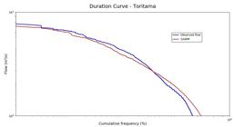
Simulated and measured flows duration curve for the Toritama streamflow gauge station, in log x log scale.

Rainfall distribution and time delay procedure

In order to address the spatial and temporal variability of the precipitations, more pronounced in semi-arid regions than in those with humid climate conditions, a procedure is used in CAWM IV to estimate the time delay until the precipitation recorded in each rain gauge will contribute to the flow at the watershed outlet. Considering the concentration time of the basin $T_c$ as the limit, this time delay is defined proportionally to the distance of each rain gauge to the main watercourse, and from there to the basin outlet. The recorded precipitations in each rain gauge are redistributed in time according to Equation 17:

$P_k^{*}\left(t\right)=P_k\left(t-i\right)$ (17)

where $P_k^{*}\left(t\right)$ is the redistributed precipitation for the data of the rainfall gauge stations inserted in the region i between isochronous in which the rain gauge is framed.

That said, the calculated precipitations are weighted by their influence areas and then the balance precipitation-evapotranspiration-infiltration-runoff proceeds through Equation 1.

The purpose of this procedure is to better represent the spatially irregular distribution of precipitations in the Brazilian semi-arid region, which is the object of the case study. In case of concentrated precipitation in areas closer to the flow measurement section, for example, the basin response in the form of runoff will occur earlier, if compared to the situation of a similar event occurred in areas farther from the control section.

As an example of the effect of rainfall irregularity, the rainy season of 2004, the highest recorded in the Pajeú river basin, was analyzed. The daily rainfall amount recorded in 77 rainfall stations was hypothetically distributed equally among: a) the 11 farthest stations from the outlet; b) the 31 nearest stations. The concentration time of PRB was calculated by Kirpich formula as being 4 days. Thus, in the case a) the precipitations contribute to the flow at the outlet on the 4^th day after its occurrence, and in the case b) their contribution is already on the first day.

The difference in the precipitation distribution is sensitive, as illustrated in Figure 11. The simulated flows, shown in Figure 12, reflect the difference in precipitation distribution.

Figure 11
Effect of different concentrations of precipitation: upper and lower PRB.

Figure 12
Flows resulting from both precipitation distribution scenarios analyzed for PRB.

This difference in the behavior of the precipitation distribution in the space is not identified in procedures that calculate the average daily rainfall, so the time delay process is applied in these cases.

Performance indicators and procedures for parameter calibration

The performance indicators used in hydrological modelling are:

$NSE$: Nash-Sutcliffe efficiency coefficient;

R²: coefficient of determination;

$RMSE$: root mean square error;

$Pbias$%: percentage of the average tendency;

$RSR$: the ratio between $RMSE$ and standard deviation.

$RMSE$, $Pbias$ and $RSR$ are calculated through the following equations:

$RMSE=\frac{1}{n}{\left[{\displaystyle \sum }_{i=1}^n{\left(Q_{i,obs}-Q_{i,cal}\right)}^2\right]}^{1/2}$ (18)

$Pbias=\left[\frac{{{\displaystyle \sum }}_{i=1}^n\left(Q_{cal}\left(i\right)-Q_{obs}\left(i\right)\right)100}{{{\displaystyle \sum }}_{i=1}^n\left(Q_{obs}\left(i\right)\right)}\right]$ (19)

$RSR=\left|\frac{{\left[{{\displaystyle \sum }}_{i=1}^n{\left(Q_{i,obs}-Q_{i,cal}\right)}^2\right]}^{1/2}}{{\left[{{\displaystyle \sum }}_{i=1}^n{\left(Q_{i,obs}-\overline{Q_{obs}}\right)}^2\right]}^{1/2}}\right|$ (20)

The Nash-Sutcliffe efficiency coefficient ($NSE$) ranges from -∞ to 1, and it can be obtained from the following equation:

$NSE=1-\frac{{{\displaystyle \sum }}_{i=1}^n{\left(Q_{i,obs}-Q_{i,cal}\right)}^2}{{{\displaystyle \sum }}_{i=1}^n{\left(Q_{i,obs}-\overline{Q_{obs}}\right)}^2}$ (21)

where $n$ is the total number of event data, $Q_{i,obs}$ is the observed flow and $Q_{i,cal}$ is the calculated flow, both in time $i$, whereas$\overline{Q_{obs}}$is the average flow observed in the period.

Several authors, such as Pushpalatha et al. (2012) and Traore et al. (2014), use $NSE$ variations, which comprises square root of flows ($NS{E}_{sqrtQ}$), decimal logarithm ($NS{E}_{logQ}$) and other derived variables, as shown in the equations below.

$NS{E}_{sqrtQ}=1-\frac{{{\displaystyle \sum }}_{i=1}^n{\left(\sqrt{Q_{i,obs}}-\sqrt{Q_{i,cal}}\right)}^2}{{{\displaystyle \sum }}_{i=1}^n{\left(\sqrt{Q_{i,obs}}-\sqrt{\overline{Q_{obs}}}\right)}^2}$ (22)

$NS{E}_{logQ}=1-\frac{{{\displaystyle \sum }}_{i=1}^n{\left(\log Q_{i,obs}-\log Q_{i,cal}\right)}^2}{{{\displaystyle \sum }}_{i=1}^n{\left(\log Q_{i,obs}-\log \overline{Q_{obs}}\right)}^2}$ (23)

The majority of the authors uses the $NSE$ as one of the main performance indicators in hydrological modelling, although there is an understanding that it should not be the only one (Schaefli & Gupta, 2007). Zappa (2002) suggests values above 0.5 for $NSE$. Gotschalk & Motovilov (2000 apud Van Liew et al., 2007) classify as very good models with $NSE$ values above 0.75 and satisfactory values between 0.75 and 0.36, whether for daily or monthly time step.

Moriasi et al. (2007) recommend evaluating the simulation performance through the ratings of the $NSE$, $Pbias$ and $RSR$ indicators as shown in Table 2 .

Table 2
Performance indicators ratings recommended for monthly simulations.

Performance rating for monthly simulations	NSE	Pbias %	RSR
Very good	0.75-1.00	< ±10	0-0.5
Good	0.65-0.75	±10 - ±15	0.5-0.6
Satisfactory	0.50-0.65	±15 - ±25	0.6-0.7
Unsatisfactory	<0.5	>±25	>0.7

• Source: Adapted from Moriasi et al. (2007).

As for Traore et al. (2014), higher $NSE$ values indicate the adjustment of higher flows, $NS{E}_{sqrtQ}$ the average flows and $NS{E}_{logQ}$ the lower flows. Pushpalatha et al. (2012) present other transformations applied to $NSE$ indicator and concluded that $NS{E}_{sqrtQ}$ is the most appropriate performance indicator to quantify the simulation adjustment with both high and low flows. In agreement with this statement, Patil & Stieglitz (2014) propose for the calibration of the parameter values in hydrological models the use of $NS{E}_{sqrtQ}$ as the objective-function.

Therefore, the objective-function used in CAWM IV Model for calibration process seeks to maximize the value of $NS{E}_{sqrtQ}$ while minimizing the absolute deviations between measured and calculated flows using Equation (24) below:

$F=\frac{NS{E}_{sqrtQ}.{10}^6}{\sum abs\left(Q_{obs}-Q_{calc}\right)}$ (24)

The CAWM IV model has been used in two versions. The first one, in the form of a MS Excel spreadsheet, uses the Solver supplement with GRG (Nonlinear Programming) or Evolutionary (Genetic Algorithm) to calibrate the parameters. In the second version, developed in Python programming, the optimization is performed through the “scipy.optimize.minimize” function which has as its calculation method the Truncated Newton Algorithm.

The GRG algorithm (Generalized Reduced Gradient) is credited to Carpentier and Abadie (Rao, 2009). The version used here is part of the M.S. Excel Solver add-in. The algorithm worked well for calibration of CAWM IV parameters, achieving convergence in up to 20 iterations. The restrictions imposed are the non-negativity of the parameters and the upper limit for parameter values $K_L$ and $K_s$ below 1.

RESULTS AND DISCUSSION

Among the watersheds for which the simulation model was applied, only in the PRB the concentration time is higher than the adopted time of 1 day. So, for PRB, before the start of the simulation, the rainfall time delay procedure was applied to redistribute in time the precipitation recorded at each station, considering its contribution proportionally lagged to the distance to the streamflow gauge station.

Regarding the performance indicators evaluated, NSE_sqrtQ was higher than 0.36 in 92% of the events (it exceeded the value of 0.5 in 79%, 0.65 in 63% and 0.75 in 44%). For NSE_logQ, the achieved values surpassed 0.5 in 80% of the events simulated. Taking into account the Moriasi et al. (2007) criteria for NSE, RSR and Pbias together, in 55% of the analyzes the adjustments were at least satisfactory (23% classified as good and 15% as very good).

Figure 13 aggregates in boxplot diagrams the results obtained for the various indicators.

Figure 13
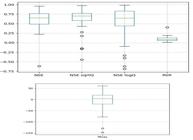
Mode value first and third quartile, and extreme values for each performance indicator used.

Considering a long-term simulation period, the model showed adequate adjustment in 100% of the studied cases, considering the set of criteria defined by Moriasi et al. (2007).

The following figures (Figure 14, Figure 15, Figure 16 and Figure 17) show some examples of the model validation.

Figure 14
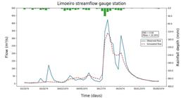
Comparison between observed and simulated discharges for Limoeiro streamflow gauge station.

Figure 15
Comparison between observed and simulated hydrographs for Santa Cruz streamflow gauge station.

Figure 16
Comparison between observed and simulated hydrographs for Caruaru streamflow gauge station.

Figure 17
Comparison between observed and simulated hydrographs for Santana streamflow gauge station.

Comparisons between CAWM IV and GR4J

In order to improve the CAWM rainfall-runoff model and for performance comparison purposes, it was applied the GR4J model – Génie Rural à 4 paramètres Journalier (Perrin et al., 2003) quoted in the introduction section of this article. Both models have in common the structure of few parameters. The goal was to compare the results between them. The GR4J also has two reservoirs, one for interception and other for storage, and its input data consists of watershed area, evapotranspiration, rain and flow data series. The model has four parameters to calibrate: X1, reservoir maximum capacity of production; X2, groundwater exchange coefficient; X3, reservoir maximum capacity of routing; and X4, base time of watershed delay hydrographs, in days (Traore et al., 2014). The cited bibliography provides more details about the model description and the equations used.

Given this information and the MS Excel spreadsheets in which the GR4J version was structured, the Pajeú and Capibaribe River basins were selected for comparison. To compare the results, the same calibration and validation periods were used in both models (Table 3).

Table 3
Calibration periods.

	Initial data	End data
Floresta	04/10/1988	06/09/1988
Limoeiro	02/10/1985	05/30/1985
Paudalho	03/03/1977	07/01/1977
Toritama	04/22/1977	05/22/1977
São Lourenço	05/01/1974	06/01/1974

The model performance was evaluated using the graphical comparison and performance indicators to determine the simulation reliability related to the observed data.

Two hydrographs examples are shown below in Figure 18 and Figure 19, referring to the events used for calibration of the Limoeiro sub-basin and the Pajeú river basin.

Figure 18
Hydrograph with Limoeiro data (Source: author, 2019).

Figure 19
Hydrograph with Floresta data (Source: author, 2019).

From the analysis of all simulations, the best efficiency indicators performances of each model in reproducing the recorded flow rates are presented in Table 4. The performance indicators used were those presented in Table 2.

Table 4
Comparison of best simulation performance.

	CAWM	GR4J
Floresta	49%	51%
Limoeiro	53%	48%
Paudalho	55%	45%
Toritama	45%	55%
São Lourenço	66%	34%

Although GR4J model has not been specifically formulated for application to semi-arid regions, the simulations have led to similar results when comparing the two models, with CAWM IV presenting slightly higher efficiency indicator percentages. Difficulty was observed to annul the recession flow with the GR4J model. While user sensitivity in calibrating with either model can always lead to better approximations, difficulty with low flow rates is common for general-purpose models. Figure 20 shows, in bilogarithmic scale, the duration curve of the simulated flows with the two models as well as the observed flows for the São Lourenço streamflow gauge station, where the indicators showed a greater difference.

Figure 20
Duration curve for observed and simulated data with both models, regarding to São Lourenço streamflow gauge station.

Evaluation of possible regionalization of the CAWM IV parameters

Table 1 presents the values of three calibrated parameters to each basin studied. To evaluate the possibility of transferring the parameter values from one basin to another, a set of parameters common to all studied basins was identified, except in case of the loss parameter. The set of these parameters was applied to long period simulation (only one with the number of years less than 21) with satisfactory results to all data series according to the criteria applied in other evaluations. The parameter values and performance indicators are presented in Table 5 below. As only one parameter differs between basins, the possibility of regionalization is considered significant.

Table 5
Regionalization parameters.

	Santa Cruz do Capibariube (SCB)	Toritama (CRB)	Limoeiro (CRB)	Paudalho (CRB)	São Lourenço da Mata (SLB)	Caruaru (IRB)	Floresta (PRB)	Santana (MRB)
Α	1.4	1.4	1.4	1.4	1.4	1.4	1.4	1.4
K S	0.0001	0.0001	0.0001	0.0001	0.0001	0.0001	0.0001	0.0001
K L	0.2204	0.2227	0.3239	0.3	0.24	0.4232	0.5312	0.5089
$NSE$	0.55	0.57	0.40	0.60	0.75	0.43	0.49	0.51
$Pbias$%	-16.22	-9.30	-17.19	-3.25	22.39	-5.13	-11.54	4.32
$RSR$	0.11	0.11	0.15	0.10	0.06	0.14	0.13	0.12
Nº of years	21	21	21	21	21	21	21	17

CONCLUSIONS

The CAWM IV lumped model was developed to better represent the physical and climatic characteristics of watersheds located in semi-arid regions and at the same time requires the calibration of a few parameters.

The CAWM IV model prioritizes the simulation of runoff, understanding that this is the most important process for studying watersheds located in semi-arid regions of shallow soils. The formulation developed to represent the runoff sought to represent the physical processes present in this stage of the hydrological cycle. Another aspect addressed concerns the spatial-temporal distribution of precipitation, which is more irregular in the semi-arid regions. The methodology used sought to better represent this issue, but it needs to be tested in basins where the precipitation-runoff lagtime is higher.

Another objective of the model is to facilitate the parameters regionalization in order to enable its application for data-scarce watersheds. The search for the integration of physical data in the parameters conceptualization allows this process.

Although the parameter calibration methods of hydrological models lead to sets with diversified values, the application to the studied basins allowed, by way of example, to determine a set of calibratable parameter values that adequately met the simulation of long-term continuous flow rates, varying only the loss coefficient. This stimulates the expectation of regionalization of parameter values on a regional scale.

The model performance for the studied basins was at least satisfactory for most simulated events. CAWM IV tests are being conducted on about 50 other watersheds in regions similar to those of the study, again comparing the performance of the model with others recognized for their use.

ACKNOWLEDGEMENTS

The authors acknowledge with gratitude the support of CNPq, CAPES, the Science and Technology Support Foundation of the Pernambuco state (FACEPE), as well as the several undergraduate students in Civil Engineering at UFPE, Campus Caruaru, especially to Hellen Vasconcelos, who have participated in the tests to improve different versions of the CAWM model. The authors also acknowledge the reviewers and editors of RBRH for the contributions that have enhanced this work.

REFERENCES

• Abbott, M. B., Bathurst, J. C., Cunge, J. A., O’Connell, P. E., & Rasmussen, J. (1986a). An introduction to the European Hydrological System — Systeme Hydrologique Europeen, “SHE”, 1: history and philosophy of a physically-based, distributed modelling system. Journal of Hydrology (Amsterdam), 87(1-2), 45-59. http://dx.doi.org/10.1016/0022-1694(86)90114-9
  » http://dx.doi.org/10.1016/0022-1694(86)90114-9
• Abbott, M. B., Bathurst, J. C., Cunge, J. A., O’Connell, P. E., & Rasmussen, J. (1986b). An introduction to the European Hydrological System — Systeme Hydrologique Europeen, “SHE”, 2: structure of a physically-based, distributed modelling system. Journal of Hydrology (Amsterdam), 87(1-2), 61-77. http://dx.doi.org/10.1016/0022-1694(86)90115-0
  » http://dx.doi.org/10.1016/0022-1694(86)90115-0
• Al-Qurashi, A., Mcintyre, N., Wheater, H. S., & Unkrich, C. (2008). Application of the Kineros2 rainfall–runoff model to an arid catchment in Oman. Journal of Hydrology (Amsterdam), 355(1-4), 91-105. http://dx.doi.org/10.1016/j.jhydrol.2008.03.022
  » http://dx.doi.org/10.1016/j.jhydrol.2008.03.022
• Al-Safi, H. I. J., & Sarukkalige, P. R. (2018). The application of conceptual modelling to assess the impacts of future climate change on the hydrological response of the Harvey River catchment. Journal of Hydro-environment Research, 1-12.
• Andréassian, V., Perrin, C., & Michel, C. (2004). Impact of imperfect potential evapotranspiration knowledge on the efficiency and parameters of watershed models. Journal of Hydrology (Amsterdam), 286(1-4), 19-35. http://dx.doi.org/10.1016/j.jhydrol.2003.09.030
  » http://dx.doi.org/10.1016/j.jhydrol.2003.09.030
• Arnold, J. G., Srinivasan, R., Muttiah, R. S., & Williams, J. R. (1998). Large area hydrologic modeling and assessment part I: model development. Journal of the American Water Resources Association, 34(1), 73-89. http://dx.doi.org/10.1111/j.1752-1688.1998.tb05961.x
  » http://dx.doi.org/10.1111/j.1752-1688.1998.tb05961.x
• Aubert, D., Loumagne, C., & Oudin, L. (2003). Sequential assimilation of soil moisture and streamflow data in a conceptual rainfall-runoff model. Journal of Hydrology (Amsterdam), 280(1-4), 145-161. http://dx.doi.org/10.1016/S0022-1694(03)00229-4
  » http://dx.doi.org/10.1016/S0022-1694(03)00229-4
• Bergström, S. (1991). Principles and confidence in hydrological modelling. Nordic Hydrology, 22(2), 123-136. http://dx.doi.org/10.2166/nh.1991.0009
  » http://dx.doi.org/10.2166/nh.1991.0009
• Bergström, S., & Lindström, G. (2015). Interpretation of runoff processes in hydrological modelling-experience from the HBV approach. Hydrological Processes, 29(16), 3535-3545. http://dx.doi.org/10.1002/hyp.10510
  » http://dx.doi.org/10.1002/hyp.10510
• Beven, K. (1989). Changing ideas in hydrology: the case of physically-based models. Journal of Hydrology (Amsterdam), 105(1-2), 157-172. http://dx.doi.org/10.1016/0022-1694(89)90101-7
  » http://dx.doi.org/10.1016/0022-1694(89)90101-7
• Beven, K. A. (2006). Manifesto for the equifinality thesis. Journal of Hydrology, 320(1-2), 18-36.
• Cabral, S. L., Sakuragi, J., & Silveira, C. S. (2017). Incertezas e erros na estimativa de vazões usando modelagem hidrológica e precipitação por RADAR. Revista Ambiente & Água, 12(1), 57-70.
• Collet, L., Ruelland, D., Borrell-Estupina, V., Dezetter, A., & Servat, E. (2013). Integrated modelling to assess long-term water supply capacity of a mesoscale Mediterranean catchment. The Science of the Total Environment, 461-462, 528-540. PMid:23756213. http://dx.doi.org/10.1016/j.scitotenv.2013.05.036
  » http://dx.doi.org/10.1016/j.scitotenv.2013.05.036
• Collischonn, W., Allasia, D., Da Silva, B. C., & Tucci, C. E. M. (2007). The MGB-IPH model for large-scale rainfall: runoff modelling. Hydrological Sciences Journal, 52(5), 878-895. http://dx.doi.org/10.1623/hysj.52.5.878
  » http://dx.doi.org/10.1623/hysj.52.5.878
• Cornelissen, T., Diekkrüger, B., & Giertz, S. (2013). A comparison of hydrological models for assessing the impact of land use and climate change on discharge in a tropical catchment. Journal of Hydrology (Amsterdam), 498, 221-236. http://dx.doi.org/10.1016/j.jhydrol.2013.06.016
  » http://dx.doi.org/10.1016/j.jhydrol.2013.06.016
• Costa, V., Fernandes, W., & Naghettini, M. (2014). Regional models of flow-duration curves of perennial and intermittent streams and their use for calibrating the parameters of a rainfall–runoff model. Hydrological Sciences Journal, 59(2), 262-277. http://dx.doi.org/10.1080/02626667.2013.802093
  » http://dx.doi.org/10.1080/02626667.2013.802093
• Dakhlaoui, H., Ruelland, D., Tramblay, Y., & Bargaoui, Z. (2017). Evaluating the robustness of conceptual rainfall-runoff models under climate variability in northern Tunisia. Journal of Hydrology (Amsterdam), 550, 201-217. http://dx.doi.org/10.1016/j.jhydrol.2017.04.032
  » http://dx.doi.org/10.1016/j.jhydrol.2017.04.032
• de Vos, N. J., Rientjes, T. H. M., & Gupta, H. V. (2010). Diagnostic evaluation of conceptual rainfall-runoff models using temporal clustering. Hydrological Processes, 24(20), 2840-2850. http://dx.doi.org/10.1002/hyp.7698
  » http://dx.doi.org/10.1002/hyp.7698
• Edijatno, M. C. (1989). Un modèlepluie-débitjournalier à trois paramètres. Houille Blanche, (2), 113-122.
• Feldman, A. D. (2000). Hydrologic modeling system HEC-HMS: technical reference manual (158 p.). USA: Hydrologic Engineering Center, US Army Corps of Engineers.
• Felix, V. S., & Paz, A. R. (2016). Hydrological processes representation in a semiarid catchment located in Paraiba state with distributed hydrological modelling. Revista Brasileira de Recursos Hídricos, 21(3), 556-569.
• Gao, C., He, Z., Pan, S., Xuan, W., & Xu, Y. (2018). Effects of climate change on peak runoff and flood levels in Qu River Basin, East China. Journal of Hydro-environment Research, 28, 34-47.
• Güntner, A., & Bronstert. A. (2003a). Large-scale hydrological modelling of a semiarid environment: model development, validation and application. In T. Gaiser, M. Krol, H. Frischkorn & J. C. Araújo (Eds.), Global Change and Regional Impacts (pp. 217-228). New York: Springer. http://dx.doi.org/10.1007/978-3-642-55659-3_17 http://dx.doi.org/10.1007/978-3-642-55659-3_17
  » http://dx.doi.org/10.1007/978-3-642-55659-3_17» http://dx.doi.org/10.1007/978-3-642-55659-3_17
• Güntner, A., & Bronstert, A. (2003b). Large-scale hydrological modelling in the semiarid northeast of Brazil: aspects of model sensitivity and uncertainty. Hydrology of the Mediterranean and Semiarid Regions, 278, 43-48.
• Güntner, A., & Bronstert, A. (2004). Representation of landscape variability and lateral redistribution processes for large-scale hydrological modelling in semi-arid areas. Journal of Hydrology (Amsterdam), 297(1-4), 136-161. http://dx.doi.org/10.1016/j.jhydrol.2004.04.008
  » http://dx.doi.org/10.1016/j.jhydrol.2004.04.008
• Hansen, J. R., Refsgaard, J. C., Hansen, S., & Ernstsen, V. (2007). Problems with heterogeneity in physically based agricultural catchment models. Journal of Hydrology (Amsterdam), 342(1-2), 1-16. http://dx.doi.org/10.1016/j.jhydrol.2007.04.016
  » http://dx.doi.org/10.1016/j.jhydrol.2007.04.016
• Hartnett, M., Berry, A., & Irvine, K. (2007). The use of modelling to implement the Water Framework Directive. WIT Transactions on Ecology and the Environment, 104, 11-20. http://dx.doi.org/10.2495/RM070021
  » http://dx.doi.org/10.2495/RM070021
• Huang, P., Li, Z., Chen, J., Li, Q., & Yao, C. (2016). Event-based hydrological modeling for detecting dominant hydrological process and suitable model strategy for semi-arid catchments. Journal of Hydrology (Amsterdam), 542, 292-303. http://dx.doi.org/10.1016/j.jhydrol.2016.09.001
  » http://dx.doi.org/10.1016/j.jhydrol.2016.09.001
• Kan, G., He, X., Ding, L., Li, J., Liang, K., & Hong, Y. (2017). Study on Applicability of Conceptual Hydrological Models for Flood Forecasting in Humid, Semi-Humid Semi-Arid and Arid Basins in China. Water (Basel), 09(10), http://dx.doi.org/10.3390/w9100719
  » http://dx.doi.org/10.3390/w9100719
• Kan, G., Zhang, M., Liang, K., Wang, H., Jiang, Y., Li, J., Ding, L., He, X., Hong, Y., Zuo, D., Bao, Z., & Li, C. (2018). Improving water quantity simulation & forecasting to solve the energy-water-food nexus issue by using heterogeneous computing accelerated global optimization method. Applied Energy, 210, 420-433. http://dx.doi.org/10.1016/j.apenergy.2016.08.017
  » http://dx.doi.org/10.1016/j.apenergy.2016.08.017
• Li, F., Zhang, Y., Xu, Z., Teng, J., Liu, C., Liu, W., & Mpelasoka, F. (2013). The impact of climate change on runoff in the southeastern Tibetan Plateau. Journal of Hydrology (Amsterdam), 505, 188-201. http://dx.doi.org/10.1016/j.jhydrol.2013.09.052
  » http://dx.doi.org/10.1016/j.jhydrol.2013.09.052
• Masafu, C. K., Trigg, M. A., Carter, R., & Howden, N. J. K. (2016). Water availability and agricultural demand: an assessment framework using global datasets in a data scarce catchment, Rokel-Seli River, Sierra Leone. Journal of Hydrology: Regional Studies, 8, 222-234.
• Mendez, M., & Calvo-Valverde, L. (2016). Assessing the Performance of Several Rainfall Interpolation Methods as Evaluated by a Conceptual Hydrological Model. Procedia Engineering, 154, 1050-1057. http://dx.doi.org/10.1016/j.proeng.2016.07.595
  » http://dx.doi.org/10.1016/j.proeng.2016.07.595
• Milano, M., Ruelland, D., Dezetter, A., Fabre, J., Ardoin-Bardin, S., & Servat, E. (2013). Modeling the current and future capacity of water resources to meet water demands in the Ebro basin. Journal of Hydrology (Amsterdam), 500, 114-126. http://dx.doi.org/10.1016/j.jhydrol.2013.07.010
  » http://dx.doi.org/10.1016/j.jhydrol.2013.07.010
• Moriasi, D. N., Arnold, J. G., Van Liew, M. W., Bingner, R. L., Harmel, R. D., & Veith, T. L. (2007). Model evaluation guidelines for systematic quantification of accuracy in watershed simulations. American Society of Agricultural and Biological Engineers, 50(3), 885-900.
• Moura, A. R. C., Montenegro, S. M. G. L., Antonino, A. C. D., Azevedo, J. R. G., Silva, B. B., & Oliveira, L. M. M. (2013). Evapotranspiração de referência baseada em métodos empíricos em bacia experimental no estado de Pernambuco – Brasil. Revista Brasileira de Meteorologia, 28(2), 181-191. http://dx.doi.org/10.1590/S0102-77862013000200007
  » http://dx.doi.org/10.1590/S0102-77862013000200007
• Nasonova, O. N. (2011). Application of a land surface model for simulating rainfall streamflow hydrograph: 2. Comparison with hydrological models. Water Resources Research, 38(3), 274-283. http://dx.doi.org/10.1134/S0097807811030080
  » http://dx.doi.org/10.1134/S0097807811030080
• Nasonova, O. N., Gusev, E. M., & Kovalev, E. E. (2011). Application of a land surface model for simulating rainfall streamflow hydrograph: 1. Model calibration. Water Resources, 38(2), 155-168. http://dx.doi.org/10.1134/S0097807811020102
  » http://dx.doi.org/10.1134/S0097807811020102
• Oudin, L., Andréassian, V., Mathevet, T., Perrin, C., & Michel, C. (2006). Dynamic averaging of rainfall–runoff model simulations from complementary model parameterizations. Water Resources Research, 42, http://dx.doi.org/10.1029/2005WR004636
  » http://dx.doi.org/10.1029/2005WR004636
• Oudin, L., Andreassian, V., Perrin, C., Michel, C., & Le Moine, N. (2008). Spatial proximity, physical similarity, regression and ungaged catchments: A comparison of regionalization approaches based on 913 French catchments. Water Resources Research, 44, http://dx.doi.org/0.1029/2007WR006240
  » http://dx.doi.org/0.1029/2007WR006240
• Oudin, L., Hervieu, F., Michel, C., Perrin, C., Andréassian, V., Anctil, F., & Loumagne, C. (2005). Which potential evapotranspiration input for a lumped rainfall–runoff model? Journal of Hydrology (Amsterdam), 303(1-4), 290-306. http://dx.doi.org/10.1016/j.jhydrol.2004.08.026
  » http://dx.doi.org/10.1016/j.jhydrol.2004.08.026
• Oudin, L., Kay, A., Andréassian, V., & Perrin, C. (2010). Are seemingly physically similar catchments truly hydrologically similar? Water Resources Research, 46, http://dx.doi.org/10.1029/2009WR008887
  » http://dx.doi.org/10.1029/2009WR008887
• Oudin, L., Salavati, B., Furusho-Percot, C., Ribstein, P., & Saadi, M. (2018). Hydrological impacts of urbanization at the catchment scale. Journal of Hydrology (Amsterdam), 559, 774-786. http://dx.doi.org/10.1016/j.jhydrol.2018.02.064
  » http://dx.doi.org/10.1016/j.jhydrol.2018.02.064
• Parajka, J., Viglione, A., Rogger, M., Salinas, J. L., Sivapalan, M., & Blöschl, G. (2013). Comparative assessment of predictions in ungauged basins – Part 1: runoff-hydrograph studies. Hydrology and Earth System Sciences, 17(5), 1783-1795. http://dx.doi.org/10.5194/hess-17-1783-2013
  » http://dx.doi.org/10.5194/hess-17-1783-2013
• Patil, S. D., & Stieglitz, M. (2014). Modeling daily streamflow at ungauged catchments: what information is necessary? Hydrological Processes, 28(3), 1159-1169. http://dx.doi.org/10.1002/hyp.9660
  » http://dx.doi.org/10.1002/hyp.9660
• Perrin, C., Michel, C., & Andréassian, V. (2001). Does a large number of parameters enhance model performance? Comparative assessment of common catchment model structures on 429 catchments. Journal of Hydrology (Amsterdam), 242(3–4), 275-301. http://dx.doi.org/10.1016/S0022-1694(00)00393-0
  » http://dx.doi.org/10.1016/S0022-1694(00)00393-0
• Perrin, C., Michel, C., & Andréassian, V. (2003). Improvement of a parsimonious model for streamflow simulation. Journal of Hydrology (Amsterdam), 279(1-4), 275-289. http://dx.doi.org/10.1016/S0022-1694(03)00225-7
  » http://dx.doi.org/10.1016/S0022-1694(03)00225-7
• Pilgrim, D. H., Chapman, T. G., & Doran, D. G. (1988). Problems of rainfall-runoff modelling in arid and semiarid regions. Hydrological Sciences Journal, 33(4), 379-400. http://dx.doi.org/10.1080/02626668809491261
  » http://dx.doi.org/10.1080/02626668809491261
• Pilz, T., Delgado, J. M., Vos, S., Vormoor, K., Francke, T., Costa, A. C., Martins, E., & Bronstert, A. (2019). Seasonal drought prediction for semiarid northeast Brazil: what is the added value of a process-based hydrological model? Hydrology and Earth System Sciences, 23(4), 1951-1971. http://dx.doi.org/10.5194/hess-23-1951-2019
  » http://dx.doi.org/10.5194/hess-23-1951-2019
• Poncelet, C., Merz, R., Merz, B., Parajka, J., Oudin, L., Andréassian, V., & Perrin, C. (2017). Process-based interpretation of conceptual hydrological model performance using a multinational catchment set. Water Resources Research, 53(8), 7247-7268. http://dx.doi.org/10.1002/2016WR019991
  » http://dx.doi.org/10.1002/2016WR019991
• Pushpalatha, R., Perrin, C., Moine, N. L., & Andréassian, V. (2012). A review of efficiency criteria suitable for evaluating low-flow simulations. Journal of Hydrology (Amsterdam), 420–421, 171-182. http://dx.doi.org/10.1016/j.jhydrol.2011.11.055
  » http://dx.doi.org/10.1016/j.jhydrol.2011.11.055
• Rao, S. S. (2009). Engineering optimization: theory and practice (4. ed., 813 p.). New York: Wiley. http://dx.doi.org/10.1002/9780470549124
  » http://dx.doi.org/10.1002/9780470549124
• Salavati, B., Oudin, L., Furusho-Percot, C., & Ribstein, P. (2016). Modeling approaches to detect land-use changes: urbanization analyzed on a set of 43 US catchments. Journal of Hydrology (Amsterdam), 538, 138-151. http://dx.doi.org/10.1016/j.jhydrol.2016.04.010
  » http://dx.doi.org/10.1016/j.jhydrol.2016.04.010
• Sarzaeim, P., Bozorg-Haddad, O., Fallah-Mehdipour, E., & Loáiciga, H. A. (2017). Environmental water demand assessment under climate change conditions. Environmental Monitoring and Assessment, 189(7), 359. PMid:28660541. http://dx.doi.org/10.1007/s10661-017-6067-3
  » http://dx.doi.org/10.1007/s10661-017-6067-3
• Schaake, J. C., Koren, V. I., Duan, Q., Mitchell, K., & Chen, F. (1996). Simple water balance model for estimating runoff at different spatial and temporal scales. Journal of Geophysical Research, D, Atmospheres, 101(3), 7461-7475. http://dx.doi.org/10.1029/95JD02892
  » http://dx.doi.org/10.1029/95JD02892
• Schaefli, B., & Gupta, H. V. (2007). Do Nash values have value? Hydrological Processes, 21(15), 2075-2080. http://dx.doi.org/10.1002/hyp.6825
  » http://dx.doi.org/10.1002/hyp.6825
• Skaugen, T., Peerebom, I. O., & Nilsson, A. (2014). Use of a parsimonious rainfall-run-off model for predicting hydrological response in ungauged basins. Hydrological Processes, 29(8), 1999-2013. http://dx.doi.org/10.1002/hyp.10315
  » http://dx.doi.org/10.1002/hyp.10315
• Tian, Y., Xu, Y., & Zhang, X. (2013). Assessment of climate change impacts on river high flows through comparative use of GR4J, HBV and Xinanjiang models. Water Resources Management, 27(8), 2871-2888. http://dx.doi.org/10.1007/s11269-013-0321-4
  » http://dx.doi.org/10.1007/s11269-013-0321-4
• Traore, V. B., Sambou, S., Tamba, S., Fall, S., Diaw, A. T., & Cisse, M. T. (2014). Calibrating the Rainfall-Runoff Model GR4J and GR2M on the Koulountou River Basin, a Tributary of the Gambia River. American Journal of Environmental Protection, 3(1), 36-44. http://dx.doi.org/10.11648/j.ajep.20140301.15
  » http://dx.doi.org/10.11648/j.ajep.20140301.15
• Van Liew, M. W., Veith, T. L., Bosch, D. D., & Arnold, J. G. (2007). Suitability of SWAT for the conservation effects assessment project: comparison on USDA agricultural research service watersheds. Journal of Hydrologic Engineering, 12(2), 173-189. http://dx.doi.org/10.1061/(ASCE)1084-0699(2007)12:2(173)
  » http://dx.doi.org/10.1061/(ASCE)1084-0699(2007)12:2(173)
• Vansteenkiste, T., Tavakoli, M., Van Steenbergen, N., De Smedt, F., Batelaan, O., Pereira, F., & Willems, P. (2014). Intercomparison of five lumped and distributed models for catchment runoff and extreme flow simulation. Journal of Hydrology (Amsterdam), 511, 335-349. http://dx.doi.org/10.1016/j.jhydrol.2014.01.050
  » http://dx.doi.org/10.1016/j.jhydrol.2014.01.050
• Wang, M., Zhang, L., & Baddoo, T. D. (2016). Hydrological Modeling in a Semi-Arid Region Using HEC-HMS. Journal of Water Resource and Hydraulic Engineering, 5(3), 105-115. http://dx.doi.org/10.5963/JWRHE0503004.
  » http://dx.doi.org/10.5963/JWRHE0503004.
• Zappa, M. (2002). Multiple-response verification of a distributed hydrological model at different spatial scales [P.hD. thesis]. Zurich: Swiss Federal Institute of Technology.

Publication Dates

• Publication in this collection
  27 Apr 2020
• Date of issue
  2020

History

• Received
  19 July 2019
• Reviewed
  22 Nov 2019
• Accepted
  11 Dec 2019