Eddy-covariance CO2 fluxes over Itaipu lake, southern Brazil

Fluxos de CO2 obtidos com o método das covariâncias turbulentas no reservatório de Itaipu, sul do Brasil

ABSTRACT

In this work, we present CO₂, latent heat and sensible heat fluxes measured over the reservoir of the Itaipu Hydroelectric Power Plant (Paraná State, Brazil) during 2013. A tower was installed at a small island in the reservoir, where an Eddy Covariance system, with supplementary equipments and analysers, was deployed. The objective of this work was to determine the magnitude of CO₂ fluxes and their variation throughout the year. CO₂ flux displayed seasonality: in warm months there was a predominance of negative CO₂ daytime fluxes and positive CO₂ nighttime fluxes, which we attributed to photosynthesis/respiration in the reservoir; in cold months there was a predominance of negative CO₂ fluxes in both periods, with CO₂ air concentration apparently imposing the signal of the CO₂ fluxes and the strong winds intensifying them. The range of 90% of the CO₂ fluxes measured in this work (−102.68 to +151.72 µg m⁻²s⁻¹ at the 30-min. time scale) is comparable to those observed in natural lakes and reservoirs around the world. On the average, the reservoir acted as a source of CO₂, with an overall mean flux of +12.78 µg m⁻²s⁻¹.

Keywords:
Reservoirs; Eddy covariance; Greenhouse gases; Itaipu power plant; CO₂ fluxes

RESUMO

Neste trabalho, apresentam-se os fluxos de CO₂, Calor Latente e Calor Sensível medidos no reservatório da Usina Hidrelétrica de Itaipu (Estado do Paraná, Brasil) durante o ano de 2013. Uma estação micrometeorológica foi instalada em uma pequena ilha do reservatório. Os fluxos de CO₂ apresentaram sazonalidade: em estações quentes havia predominância de fluxos de CO₂ negativos de dia e positivos à noite, que nós atribuímos à fotossíntese/respiração no reservatório; em estações frias os fluxos eram na maior parte das vezes negativos em ambos os períodos, com a concentração de CO₂ no ar aparentemente impondo o sinal dos fluxos de CO₂ e ventos fortes intensificando eles. 90% dos fluxos de CO₂ medidos neste trabalho (−102,68 a +151,72 µg m⁻²s⁻¹ na escala de tempo de 30-min.) variaram em um intervalo comparável aos fluxos medidos em lagos naturais ao redor do mundo. Em média, o reservatório agiu como uma fonte de CO₂, com um fluxo médio de +12,78 µg m⁻²s⁻¹.

Palavras-chave:
Reservatórios; Método das covariâncias turbulentas; Gases de efeito estufa; Usina Hidrelétrica de Itaipu; Fluxos de CO₂

INTRODUCTION

In the last decades, continental water bodies have been found to be potentially important sources of greenhouse gases to the atmosphere. In particular, reservoirs of hydroelectric plants have been under intense scrutiny since the work of Rudd et al. (1993), which for the first time presented evidence that they could be important sources of CO₂ and CH₄.

Currently, the overall carbon balance of lakes and reservoirs remains subject to considerable uncertainty, and their role as sources or sinks in the carbon cycle remains, to a large extent, unknown (Huotari et al., 2011; Mendonca et al., 2012). In several cases, reservoirs and lakes have been reported to be large accumulators of carbon in their sediments (Tranvik et al., 2009; Mendonca et al., 2012; Ometto et al., 2013; Bernardo et al., 2017). As sources of atmospheric CO₂ and CH₄, however, there is comparatively less uncertainty: most studies generally report net carbon dioxide and methane emissions into the atmosphere through the water surface of freshwater ecosystems (Rosa et al., 2003; Soumis et al., 2004; Kemenes et al., 2011; Huotari et al., 2011; Mammarella et al., 2015; Erkkilä et al., 2018) and, in the case of hydropower reservoirs, as a result of “degassing” as well (the process of ebullition of CH₄ and CO₂ as the water pressure drops suddenly downstream of the turbines) (Galy-Lacaux et al., 1997; Soumis et al., 2004).

Clearly, the subject of carbon balance of lakes and reservoirs is a complex one, and considerable efforts will be needed before a more definitive picture of their overall contribution to emission and sequestration of carbon, in its various forms, can be reached. In this work, we adopt as an assumption that CO₂ fluxes across water surfaces fluctuate over time in sequences of positive and negative values according to local drivers. With no a priori assumption about the reservoir role (if it is a source or a sink of CO₂), we will concentrate on the question of quantifying CO₂ exchanges across the water surface of a large subtropical reservoir by means of the eddy covariance (EC) method.

The EC technique is widely accepted for the measurement of greenhouse gas (GHG) fluxes at the ecosystem scale: it has been applied to all kinds of terrestrial ecosystems (Xu & Baldocchi, 2004; Lewicki et al., 2007; Suni et al., 2003; Hatala et al., 2012). For water bodies, however, its application is more difficult due, among other factors, to the requirement of a stable measuring platform, power supply and logistical difficulties. This partly explains the choice of the chamber method and the mass-transfer method (which requires measuring the partial pressure of CO₂ in water, usually by means of an analytical water-air equilibration approach, and in the air), which are relatively simple to apply (Kutzbach et al., 2007; Paranaíba et al., 2018), as the principle measuring techniques in water body studies of GHG emissions (Rosa et al., 2003; Zhu et al., 2012; Ometto et al., 2013; Abril et al., 2014; Pacheco et al., 2015). However, floating chambers have been criticized for causing modification of the flow at the water-air interface (Richey et al., 2002; Schubert et al., 2012). Another limitation is that point measurements in space and time of these methods need to be extrapolated for the whole water body, and are sometimes used to obtain estimates of long-term average GHG fluxes (Vesala et al., 2006; Podgrajsek et al., 2014; Paranaíba et al., 2018).

In Brazil, there has been a considerable effort to estimate GHG emissions from the reservoirs of hydroelectric plants (dos Santos et al., 2006; Kemenes et al., 2011; Ometto et al., 2013; Marcelino et al., 2015; Vale et al., 2017), partly due to their importance in the country’s energy generation matrix: 60.3% of Brazil’s electrical power are produced by hydroelectric plants (Empresa de Pesquisa Energética, 2018). The magnitudes of the net emissions of greenhouse gases to the atmosphere reported in those studies varied significantly: for example, Kemenes et al. (2011) estimated fluxes of 2.9 ton C/MWh from the Balbina hydroelectric reservoir. In comparison with a baseline emission per MWh from an equivalent coal powered thermoelectric plant (0.3 ton C/MWh), Balbina would emit almost ten times more GHG per MWh. On the other hand, Ometto et al. (2013) reported much lower emissions from 8 Brazilian hydropower reservoirs: their emissions varied from 0.01 to a maximum of 0.55 ton C/MWh, with only two reservoirs having emissions comparable to a thermal powerplant. All those studies resorted to the chamber method. The limitations of the chamber method were discussed above, and were present in those studies as well: temporal coverage was limited; seasonality had to be inferred from sparse measurements; and the measurement campaigns were limited by weather conditions (the method can’t be used under high winds, for example (Mannich et al., 2017)).

In contrast to chamber measurements, the EC method allows direct measurement of the turbulent flux on a continuous basis. The technique is non-intrusive and the measurement is representative of a region upwind of the measuring tower which is of the order of a few hundred meters, called the “footprint” (Schuepp et al., 1990).

In this work, we present 11 months of CO₂ flux measurements (with gaps: 149 days in total) at a large reservoir of a hydroelectric plant in Southern Brazil (Itaipu). The main objective is to quantify the fluxes of CO₂ across the water surface. Fluxes of sensible and latente heat were also measured and are briefly described as they are needed for the calculation of atmospheric stability and density corrections. We apply a footprint-based methodology to select the fluxes which come exclusively from the water surface in a reservoir where the water level fluctuates. The measurements allowed to determine the seasonality of CO₂ fluxes at the Itaipu reservoir, with the lake functioning mostly as a source of CO₂ to the atmosphere.

METHODS

Site and measurements

Itaipu reservoir is located in the valley of the Paraná River, at the border between Brazil and Paraguay. The reservoir reached its normal operating level at the 220-m elevation (above mean sea level) for the first time in June 1984. At this level, the lake has a surface area of 1350 km².

The drainage basin formed between the Itaipu dam and the previous dam located approximately 400 km upstream from it on the same river (Sérgio Motta Hydroelectric Power Plant) has an area of 147000 km². This area presents three main types of land use: natural forests (∼ 12%), agriculture (∼ 48%) and pasture (∼ 40%) (Brasil, 2014). Most of the forested area is concentrated on the Western margin (Paraguayan), but a 30-m wide belt of reforestation exists along the Eastern (Brazilian) margin as well. Deciduous trees characterize the forest in this area. Crops are found on both sides of the lake.

A small micrometerological tower was set up on a flat, almost submerged, hill top (latitude −25^◦03ˈ25.72”; longitude −54^◦24ˈ33.67”; and altitude 218 m ASL). Note that the hill top is two meters below the normal operating level. At lower water levels, a small island appears. This provides very good conditions for EC measurements, with a fetch of 3000 m to the North, 1500 m to the West, 2000 m to the South and 500 m to the East (see Figure 1). In Figure 1 we also plotted an approximation of the reservoir’s bed surface around the EC station, downloaded from Instituto de Terras Cartografia e Geociências do Paraná (2020).

Figure 1
Location of the eddy covariance station and an approximation of bed surface of Reservoir. The site’s island is very small and is represented by the black dot at 218 m ASL on the right panel.

At the EC station, a sonic anemometer (Campbell Scientific Instruments - CSI CSAT3), an infrared CO₂ and H₂O analyzer (Licor LI-7500), and four thermocouples (CSI FW03) were installed to make high-frequency (20 Hz) turbulence measurements. The thermocouples were installed above, below and in the center of the sonic path, and in the center of the optical path of the infrared analyzer. The sensors were deployed on a small metal tower and placed at 3.76 m above the ground (Figure 2).

Figure 2
Photograph of the micrometeorological station on the island of the Itaipu reservoir.

Low-frequency measurements (0.1 Hz) were also made of mean CO₂ concentration (Vaisälä GMP343; two at 1.77 m and two at 3.66 m); mean temperature and relative humidity (CSI CS500; at 2.85 m); mean atmospheric pressure (CSI CS100; at 1.73 m); mean downwelling solar radiation (Kipp & Zönen; at 2.67 m) and rainfall intensity (MRI; at 3.00 m). The pluviometer suffered frequent clogging by wasp nesting, and daily data from a nearby land station (Itacora station operated by Águas Paraná, located at latitude 25^◦06ˈ33.99” and longitude 54^◦23ˈ58.99”) was used to detect rainfall periods for quality control of the LI-7500 measurements. To measure water temperature we installed two CSI L108 temperature sensors in a nautical buoy (Alcântara et al., 2013) moored 3 km northwest of the EC site (see Figure 1) at the surface (skin surface temperature) and 25 cm below the water level. Although it was planned to measure several variables at the buoy, including pH, a lightning strike interrupted its measurements soon after our micrometeorological station was set up (note that the water temperature measurements were independent of the rest of the sensors at the buoy, and proceeded without problems). Although there are no simultaneous measurements (other than water temperature) at the buoy and the micrometeorological station, we used the water pH measured at the buoy from July to November 2012 to help to interpret some of our CO₂ flux observations in 2013 (data available at SIMA (Sistema Integrado de Monitoramento Ambiental, 2020)) (see sections 3.4 and 4).

All the high-frequency raw turbulence measurements were made continuously and stored in a computer’s disk running at the site, except for power interruptions, when the solar panels were not able for some reason to recharge the batteries, in 10-minute data files. The low-frequency data were stored as 10-min. averages. We call the 10 min. measurement periods “blocks”. Non-continuous measurements proceeded from December 2012 through April 2014. After July 2013, a robust power supply system was installed that increased the number of days with data collection considerably. The measurements presented in this work are from January to November 2013. Table 1 shows the beginning and end of each measurement period when the station was actively measuring, as well as the total number of blocks for those periods and the total number of blocks selected in a quality control process described in the next section.

Table 1
Periods during which the micrometeorological station was operating, its corresponding total of 10-minute blocks and the total number of blocks selected in a quality control (Q.C.) process. Times are in local time (LT) (local time = UTC - 3).

Period	Beginning	End	# 10-min. Blocks	# Blocks after Q.C.
I	23/01/2013 1040LT	25/01/2013 0910LT	282	171
II	27/02/2013 1110LT	05/03/2013 1650LT	789	498
III	13/03/2013 0000LT	20/03/2013 0420LT	969	630
IV	04/04/2013 1940LT	13/04/2013 1700LT	882	540
V	24/07/2013 0120LT	08/08/2013 1540LT	1782	1131
VI	08/08/2013 1710LT	04/09/2013 1520LT	3126	2028
VII	05/09/2013 0840LT	08/10/2013 1520LT	3489	2280
VIII	09/10/2013 1000LT	08/11/2013 0840LT	3666	2334
IX	08/11/2013 1000LT	23/11/2013 2200LT	2022	1287
X	24/11/2013 0000LT	30/11/2013 1500LT	705	432

Eddy covariance data processing and analysis

In a first round of data quality control, we eliminated spikes from the blocks by removing points lying outside the interval defined by five times the standard deviation (±5σ) around a 5-minute average from a linear autorecursive filter (the linear filtering is easier to implement, and computationally faster, than a centered running average) (Vickers and Mahrt, 1997). If the total number of spikes in each block was less than 50, the resulting gaps were filled with the mean from each run; otherwise, the quality control criterion was to eliminate it from further analysis. We also corrected the time lag between CSAT3 and LI-7500 sensor measurements, with the finewire thermocouple placed in the middle of the LI-7500 path. The CO₂ concentration data were shifted by an amount corresponding to the peak of the cross-correlation function between temperature and CO₂ fluctuations, for each run. The same procedure was done between temperature and vertical velocity. This methodology corrects the delay in the internal processing of the sensors and the loss of covariance generated by the spatial separation between CSAT3 and LI-7500 (Qi et al., 2015).

In addition, we grouped three consecutive 10-minute blocks to get the CO₂ fluxes from 30-minute blocks. In a procedure similar to that established by Vickers & Mahrt (1997), to select stationary 30-minute blocks, we calculated CO₂ fluxes whose CO₂ kinematic fluxes of the 30-minute block ($F_{30}$) and its 10-minute sub-blocks ($F_{10}$) were in the range of $\left|F_{30}-F_{10}\right|<\left(5\text{\%}\right)F_{30}$. The above-mentioned quality control procedures selected the number of blocks from each of the measurement periods shown in Table 1, column 5.

A 2-D rotation (Finnigan et al., 2003) was applied to each 10-min. block that passed the quality control process to align the x axis with the mean wind direction and to set the mean vertical wind velocity to zero. The fluctuations were extracted after linear detrending (Moncrief et al., 2004) over each 10-min. block.

Before the beginning of the experiment, the zero and span of the LI-7500 were adjusted per the manufacturer’s instructions. After this, the sensor was deployed in the micrometeorological station, where was kept during the whole campaign. The remoteness and access conditions of the site made field calibration difficult. Thus, we used a very stable slow-response GMP343 as a surrogate standard. The adopted procedure is described in full in Armani (2019) and Armani et al. (2020) and consists of correcting the LI-7500 CO₂ measurements with multiple regressions adjusted to the data from each of the periods in Table 1, but for daytime and nighttime periods separately. We used auxiliary mean (10 min.) meteorological observations of temperature (θ), water vapor concentration (ρ_v) and atmospheric pressure (p) to correct the LI-7500 CO₂ measurements (ρ_c,l) as follows: based on the assumption that GMP343 measurements converted to CO₂ mixing ratios are correct (r_c,g), we calculated the linear regression

$\delta r_{c,g}={\alpha }_1\delta {\rho }_{c,l}+{\alpha }_2\delta \theta +{\alpha }_3\delta {\rho }_v+{\alpha }_4\delta p$ (1)

to obtain turbulent fluctuations of CO₂ mixing ratios with

$r_c^{\text{'}}={\alpha }_1{\rho }_{c,l}^{\text{'}}+{\alpha }_2{\theta }^{\prime }+{\alpha }_3{\rho }_v^{\text{'}}$ (2)

In Equation 1, the δa’s are obtained from $a\text{'}=a+\delta a$, where a is any of the variables r_c,g, ρ_c,l,, θ, ρ_v and p; $a\text{'}$ is the mean of the 10-minute blocks and $a$ is the average of the a measurements during the whole period, but calculated separately for daytime and nighttime. Turbulent CO₂ fluctuations were grouped in 30-minute samples to obtain CO₂ fluxes with

$F_c=\overline{{\rho }_d}\overline{w^{\prime }{r}_c^{\text{'}}}$ (3)

where $\overline{{\rho }_d}$ is 30-min. mean dry air density and $w^{\prime }$is the turbulent fluctuation of vertical velocity. The procedure outlined above for the calculation of F_c was carefully checked under the assumption of perfect calibration, where it was shown to produce identical results to the WPL correction applied separately to 10-min. data blocks.

Water vapor fluxes (E) were corrected with the WPL correction (Webb et al., 1980),

$E=\left(1+{\mu }_v\overline{r_v}\right)\left(\overline{w^{\prime }{\rho }_v^{\text{'}}}+\overline{{\rho }_v}\frac{\overline{w\text{'}\theta \text{'}}}{\overline{\theta }}\right)$ (4)

and sensible heat fluxes were obtained from

$H=\overline{\rho }{c}_p\overline{w\text{'}\theta \text{'}}$ (5)

In Equations (4)–(5) $c_p$ is the specific heat of air, $\overline{\rho }$ is the mean density of air and ${\mu }_v$ is the ratio of the molecular weights of dry air to water vapor. To obtain the latent heat fluxes (LE), we multiplied E by the latent heat of vaporization: L = 2462 kJ kg^-1. In (2)–(5), all variables obey a Reynolds decomposition, with overbars denoting mean quantities, and primes denoting turbulent fluctuations.

For some periods, the reservoir’s water level was low enough to render above water a significant amount of land in the island over which the EC station was installed. Therefore, we obtained an estimate of the expected contribution of this land surface to the fluxes measured by the tower. To take into account the heterogeneous footprint we used the analytical 1-D model (along the wind direction) of Hsieh et al. (2000),

$f\left(x,z_m\right)=\frac{1}{k^2{x}^2}D{z}_u^P{\left|L\right|}^{1-P}exp\left(\frac{-1}{k^{2}x}D{z}_u^P{\left|L\right|}^{1-P}\right)$ (6)

(with a cross-wind gaussian distribution as proposed by Gryning et al. (1987)), where $k=0.4$ is von Kármán’s constant, D and P are constant over different stability ranges (see Table 2), and $z_u$ is given by

$z_u=z_m\left[ln\left(\frac{z_m}{z_0}\right)-1+\frac{z_0}{z_m}\right]$ (7)

where $z_m$ is the height of the measurements above water (which varies over time), and $z_0$ is the momentum aerodynamic roughness length of the surface.

Table 2
Values of D and P in Equation 6.

Stability	D	P
unstable	0.28	0.59
neutral	0.97	1.00
stable	2.44	1.33

When the water surface level is above 219 m ASL, the island is essentially flooded, and the EC footprint is all over water. A corresponding $z_0=0.0001$m was used in these situations (Panofsky & Dutton, 1984). Whenever the water level was below 219 m ASL, an effective roughness that took into account the heterogeneous footprint of water and the land surface of the island was calculated iteratively using the method proposed by Hutjes et al. (2010),

$z_{0ef}=e^{\frac{1}{n}{{\displaystyle \sum }}_{i=1}^{n}ln\left(z_{0i}\right)},$ (8)

with $z_0=0.0001$ m for water and $z_0=0.05$ m for the land over the island (Panofsky & Dutton, 1984), with the index i, which selects water or land, running over each grid of the discretization of the footprint along the wind direction. The procedure clearly needs to be iterative, as the contribution of water and land to the footprint depends of $z_{0ef}$, but converges quickly.

RESULTS

Footprint analysis

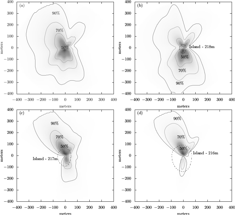
From Figure 1, it is seen that the closest distance from the island to the reservoir’s margin is approximately 500 m to East. Overland distances from the EC sensors to the water are 95, 140, 70 and 93 m to the North, South, East and West at the lowest 216-m water level. A composite shape, made up from 3 ellipses, that grows linearly with water level was adopted to represent the island’s contour, and is depicted as a dashed line in Figure 3. In that figure, we show the footprint contours for the runs obtained after quality control for the water-level ranges: (a) above 219 m; (b) 218-219 m; (c) 217-218 m and (d) 216-217 m.

Figure 3
Average flux footprint for the periods with water levels in the ranges: > 219m (a), 218-219m (b), 217-218m (c) and 216-217m (d).

In Figure 3, the lines show the 90%, 70% and 50% footprint contours, whereas the dashed line indicates the island’s contour at the lowest water level of the range. Notice that this gives a conservative view of the contribution of the land surface.

Most of the measurements were made while the water level was above 219 m, totaling 58.61% of the blocks. 25.02% of the blocks were measured while the water level range was 218-219 m; 13.43% in the range of 217-218m; and only 2.94% bellow 217m. The footprint analysis shown in Figure 2 clearly indicates that the EC tower does not “see” fluxes from the mainland (the footprint does not reach the margins of the reservoir), but that there is considerable flux from the island itself for the ranges of 216-217 and of 217-218m (Figures 22d). Thus, we removed all the measurements made when the water level was below 218m. This eliminates a further 16.37% of the fluxes that passed all the quality control procedures described above. The number of remaining runs after the footprint analysis for each month is listed in Table 3.

Table 3
Percentage of turbulent fluxes (H, LE and F_c) remaining after the Footprint Analysis (F.A.).

Period	% fluxes after F. A.	Period	% fluxes after F.A.
I	0	VI	100
II	63.3	VII	100
III	38.6	VIII	100
IV	100	IX	47.1
V	100	X	0

Meteorological variables and water surface temperature

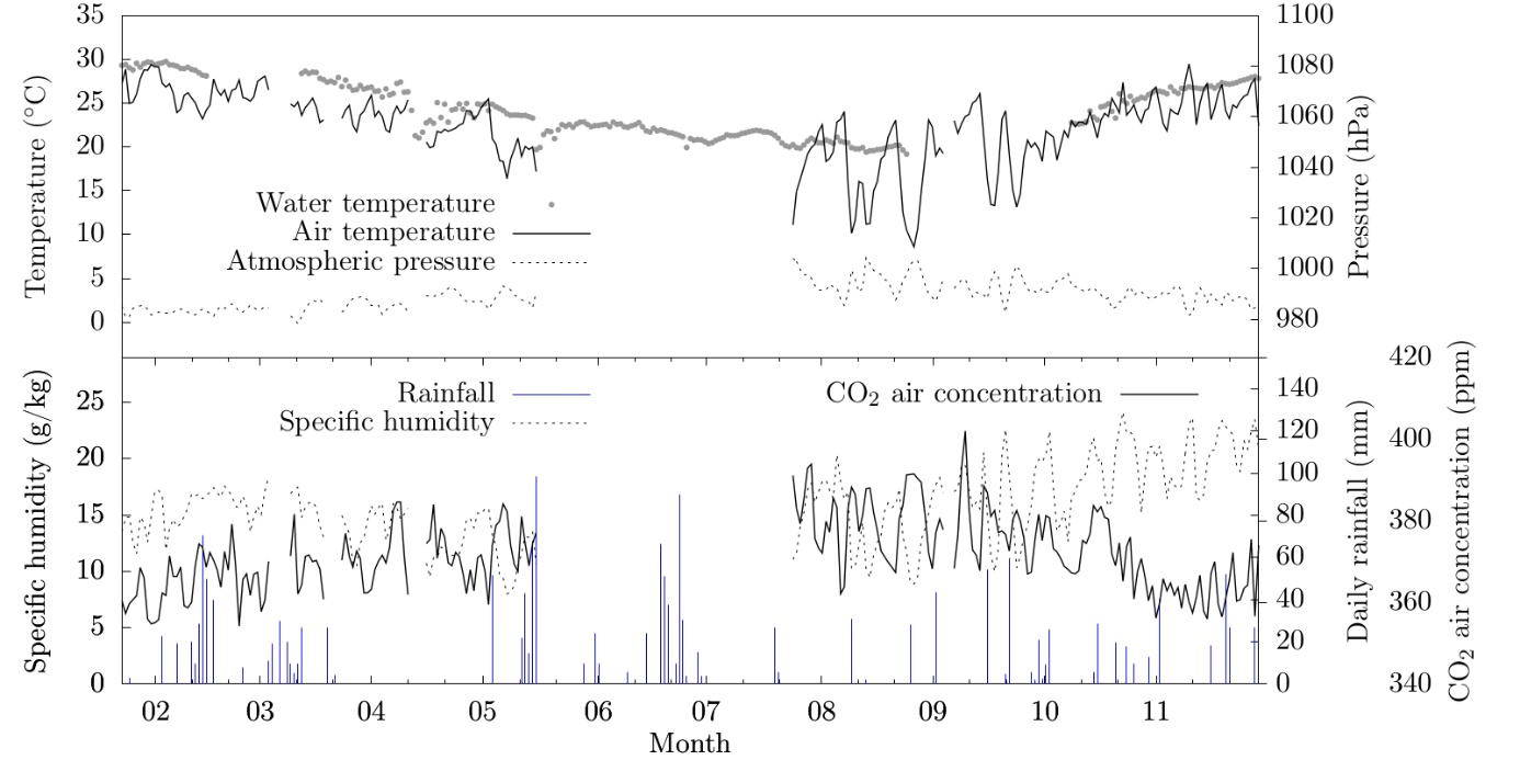
In Figure 4 we show the daily means of water surface temperature, air temperature, atmospheric pressure, specific humidity and CO₂ air concentration, as well as daily rainfall. Interruptions of plotted lines or data points indicate the periods when the sensor in question was not operating.

Figure 4
Daily averages of water temperature, air temperature, pressure and relative humidity, and daily accumulated rainfall.

Daily mean air temperatures are in the range of 10-30 °C most of the time, and surface water temperature varies much less, as expected, in the range of 20-30 °C. Data are missing for most of the wintertime, but during springtime there are large temperature fluctuations in phase with opposite atmospheric pressure fluctuations associated with the passage of weather systems. Figure 4 also shows that air CO₂ concentration is higher in colder months than in warmer months, suggesting the effect of a lower biological activity related to photosynthesis both in the water and on the surrounding land. The effect of air density variation on CO₂ concentrations is also quite clear in this figure, since this concentration varies with air temperature, especially in the abrupt variations measured in August and September.

Wind roses for daytime and nighttime, for all the data available after quality control and footprint analysis are shown in Figure 5. They are not too different, with more westerly winds during the night. There is a very low frequency of winds coming from the East, which is the direction closest to the margin (c.f.Figure 1), therefore assuring that the measurements are highly representative of the water surface. The most frequent directions reflect the topographical effect of the reservoir’s orientation.

Figure 5
Wind rose for daytime hours, left, and nighttime, right.

Sensible and latent heat fluxes

The overwhelming majority of measurements were made in the range of −1 ≤ ζ ≤ +1, where ζ is Obukhov’s stability variable, which is fairly typical of stability conditions found in the surface layer. Furthermore, most measurements were performed under unstable atmospheric conditions, totaling 58.5% of all measurements.

The hourly means of the H and LE fluxes over each period are shown in Figure 6a and b. Note that the total number of available runs is different for each month, which affects the accuracy of the averages shown. Still, Figure 6 provides a convenient way to summarize flux patterns. The most noteworthy features of H are its low values in comparison to those over land surfaces (typical of water surfaces), and that it is most often positive during daytime, with negative values occurring during nighttime and in the late afternoon in some months. On the average, LE is positive throughout the 24-hour period, with the highest values occurring in daytime around noon, sometimes with a second peak in the afternoon.

Figure 6
Hourly averages of sensible heat flux (H) and latent heat flux (LE) from measurement periods.

CO₂ fluxes: daily and seasonal variation

In Figures 7, 8 and 9 we show three 4-day periods of measurements in detail (hereafter named Sample Period 1, 2 and 3, respectively) reasonably representative of the CO₂ patterns observed throughout the experiment. Sample Period 1 extends over March 13-17 (in Period III); during this period, we observe diurnal CO₂ uptake and nocturnal CO₂ emission, suggesting that photosynthesis and respiration are driving CO₂ concentrations in water. Sample Period 2 extends over July 27–31 (in Period V), and represents the somewhat unexpected pattern of nighttime CO₂ uptake and daytime emission. Sample Period 3, during August 12-16, belongs to Period VI, and intense winds generated fluxes of greater magnitude. In Figures 7, 8 and 9 we show the observed interplay of several environmental variables: surface water and air temperature at 3.76 m, atmospheric pressure, solar radiation and CO₂ concentration at 3.66 m, sensible (H) and latent (LE) heat fluxes, wind speed and direction, and CO₂ fluxes.

Figure 7
Sample Period 1, period representative of photosynthesis/respiration driven CO₂ fluxes. LE and H are latent and sensible heat fluxes, respectively.

Figure 8
Sample Period 2, CO₂ concentration driven CO₂ fluxes. LE and H are latent and sensible heat fluxes, respectively.

Figure 9
Sample Period 3, high winds intensifying CO₂ fluxes magnitude. LE and H are latent and sensible heat fluxes, respectively.

As already mentioned above, in Figure 7, negative CO₂ fluxes are driven by photosynthesis. During this period water temperature is greater than air temperature, with larger sensible heat fluxes during daytime. The solar radiation intensity of the Sample Period 1 is higher compared to the other periods selected for this section: Figure 7 shows the solar radiation reaching 800 W m⁻², while in Figures 8 and 9 the maximum solar radiation is 600 W m⁻². Note in Figure 7 the strong daily variation in CO₂ concentration in the atmosphere, which is probably a consequence not only of the CO₂ fluxes from the water surface, but also of the land CO₂ fluxes around the reservoir.

Episodes of daytime CO₂ emission and nighttime CO₂ uptake by the reservoir were common in July (Figure 8). It is noted that the fluxes during this period are smaller (in absolute value) than the fluxes during the other two periods (all of F_c, H and LE).

During Sample Period 3, Figure 9, strong winds are observed, which generated larger fluxes. Note the drop in air temperature by approximately 14^◦C between 13th and 15th Aug and the increase in atmospheric pressure during this period, showing the passage of a climate system.

In theory, under ideal conditions, CO₂ fluxes depend on the CO₂ concentrations in air and water. Unfortunately, there were no measurements of CO₂ in the water during the experiment to assess the CO₂ water-air concentration difference. However, continuous water pH measurements performed from July to November 2012 at the buoy showed in Figure 1, indicate the existence of pH seasonality and a daily pH cycle.

In Figure 10 we selected two periods of 2012 with solar radiation patterns roughly analogous to those of Sample Periods 1 and 2: In the October 2012 14-20 period (analogous to Sample Period 1), the water pH displayed a marked daily cycle, ranging from 7.7 to 8.7, which corresponds to daytime CO₂ uptake and nighttime emission, with the pH increasing during the day and decreasing at night. In the July 30 – August 05 period (analogous to Sample Period 2), the water pH varied over a much smaller range (7.0–7.5) and there was no discernible daily cycle. This suggests that the CO₂ concentration in water was approximately constant during this period.

Figure 10
In (a) and (b) are the 2012 periods representatives of the higher and lower incoming solar radiation, respectively, and the corresponding pH variation.

Table 4 shows the corresponding CO₂ flux values as well as the values of the main flux drivers (solar radiation, wind speed and CO₂ air concentration) averaged over each measurement period. The CO₂ flux drivers clearly influenced the sign of the average CO₂ flux in periods II to IX, as shown in Table 4. In period V, for example, we observed the highest mean CO₂ concentration in the air, the second highest mean wind speed, and a negative CO₂ mean flux during both daytime and nighttime. In periods III, VII and VIII, when solar radiation was only lower than in periods II and IX, the mean daytime CO₂ fluxes were negative, probably due to photosynthesis. Despite the higher solar radiation of periods II and IX compared to other periods, the mean concentrations of CO₂ in the air were the lowest of all periods, favoring positive CO₂ fluxes.

Table 4
Period averages of nighttime, daytime and 24h CO₂ fluxes, and of their main drivers (solar radiation, wind speed and CO₂ air concentration).

Period	CO2 fluxes			Solar Radiation	Wind speed	CO2 air concentration
	24h	Nighttime	Daytime
	µg m−2s−1	µg m−2s−1	µg m−2s−1	W m−2	m s−1	ppm
II	+44.06	+71.34	+16.77	237.02	2.64	375.47
III	−0.06	+31.00	−31.11	154.65	2.78	377.20
IV	+16.30	+35.41	−2.82	123.06	2.63	381.20
V	−14.76	−25.13	−4.38	142.58	6.18	381.46
VI	+19.57	+8.50	+30.63	138.68	6.83	377.93
VII	+7.07	+32.26	−18.13	163.78	1.07	379.00
VIII	+21.07	+62.62	−20.48	155.03	1.31	378.20
IX	+19.78	+34.69	+4.86	222.44	1.20	374.45

The pattern of the observed CO₂ fluxes during 2013, in Figure 11, clearly shows their seasonality. The mean of all fluxes measured in daytime was −0.07 µg m⁻²s⁻¹, and +25.62 µg m⁻²s⁻¹ in nighttime. The overall mean was +12.78 µg m⁻²s⁻¹. The nighttime fluxes of periods V and VI indicated CO₂ uptake in the reservoir and approximately zero fluxes, respectively. The daytime fluxes measured in periods IV, V and IX also showed approximately null average fluxes.

Figure 11
Period average of nighttime, daytime and 24h CO₂ fluxes.

DISCUSSION

The observations of CO₂ flux as a function of wind direction are shown in Figure 12, where they are further classified according to daytime or nighttime. The good fetch conditions for most directions, already noted in Figure 3, are confirmed, with very few measurements coming from East, which is the direction closest to the margins. Also noteworthy is the specific pattern of negative (absorption) and positive (emission) values of the fluxes: for example, as already observed, there are many situations of negative fluxes during nighttime. This is very different from a land environment, where most nighttime fluxes are positive due to the absence of light for photosynthesis. This is strong evidence, also, that our measurements are not being affected by local advection from the margins, where both tall vegetation and agricultural fields can be found.

Figure 12
(a) Number of runs and (b) individual values of CO₂ fluxes, as a function of wind direction. W (West), N (North), E (East).

It is well known that the water pH responds to the CO₂ concentration in water: when CO₂ is absorbed in water, water pH decreases, and vice-versa (Potes et al., 2017). If the water pH in 2013 displayed the same pattern as observed 2012 (under similar radiation forcings) in the Itaipu reservoir, our hypothesis is that in the periods with higher incoming solar radiation (such as in Sample Period 1), photosynthesis removes CO₂ from the water during daytime and respiration replenishes it at night, resulting in the variation of pH shown in Figure 10a. Thus, the CO₂ water concentration contributed to the CO₂ concentration difference between water and air, producing larger (in absolute value) CO₂ fluxes. In periods of lower incoming solar radiation, such as in Sample Period 2, the water pH varies considerably less, and this suggests that the CO₂ water concentration varies less as well. This variation between the CO₂ concentration and pH in the water is a commonly reported pattern in the literature, as shown by Finlay et al. (2009) in freshwater bodies and Duarte et al. (2008) in saline lakes. Therefore, in Sample Period 2 apparently the CO₂ fluxes are mainly forced by the variation of CO₂ concentration in air. Observe in Figure 8 that CO₂ fluxes vary in opposite phase to the CO₂ concentration in the air, which justifies the negative nighttime CO₂ fluxes in Sample Period 2: the higher the CO₂ concentration in the air, the more negative the CO₂ fluxes are and vice-versa. Eugster et al. (2003) also found nighttime negative CO₂ fluxes, but they argued that these fluxes were not from the lake, because they were measured during extremely stable atmospheric conditions and CO₂ concentrations in the lake were greater than atmospheric concentrations. Differently from Eugster et al. (2003), during Sample Period 2, although most of the CO₂ negative fluxes were measured at low wind speeds, the measurements took place under unstable atmospheric conditions.

We also observed some periods with high wind speed intensifying the turbulent fluxes. According to Liu et al. (2016), synoptic events may increase the mixing of the water column by both convection and the mechanical mixing of water by wind. In fact, ultimately the scalar fluxes are intensified by wind speed, as shown for CO₂ fluxes by Macintyre et al. (2013) and for energy fluxes by Blanken et al. (2000). As discussed in McGillis et al. (2001), the gas transfer rate between water and air is higher under high wind conditions, probably due to the thinning of the diffusive layer of the water surface, as well as due to the increased turbulence in the water column. We must however emphasize that the foregoing discussion is qualitative, and that more research into the subject is needed, with simultaneous and continuous measurements of CO₂ flux and CO₂ concentration both in water and in the air.

With the exception of the winter periods (periods V and VI), the nighttime fluxes were all larger than the daytime fluxes (Table 4). Liu et al. (2016) also found higher nocturnal fluxes than daytime fluxes in a freshwater reservoir. They showed that CO₂ fluxes measured over a year with Eddy Covariance at the Ross Barnett Reservoir, located in Mississippi State - USA, were approximately 70% higher than those measured during the day.

The emission of CO₂ from continental waters is a consequence of CO₂ surface water saturation, generated by the biological respiration of organic carbon. Generally, the main source of organic carbon in reservoirs is allochthonous (Bernardo et al., 2017), but this depends on the age of the reservoir. As shown by Barros et al. (2011), newly implanted reservoirs emit more greenhouse gases due to the biodecomposition of organic matter from the flooded areas. Over time, the concentration of this organic matter decreases, driving down the emission of greenhouse gases as well. According to Teodoru et al. (2011), only in the first 15 years of the reservoir the main source of carbon is the flooded biomass. Therefore, since the Itaipu reservoir has been in existence since 1984, it is very likely that the greenhouse gases are generated mainly by allochthonous carbon.

During 2012, the Balcar (Brasil, 2014) project measured the diffusion fluxes of CO₂ from the Itaipu reservoir using the chamber method at 45 points distributed throughout the reservoir surface. These points were sampled four times in measurement campaigns that took place in January, May, August and October 2012. The CO₂ fluxes deemed representative of the reservoir ranged from approximately +3.47 µg m⁻²s⁻¹ to +16.20 µg m⁻²s⁻¹ (Brasil, 2014), which encompasses the average CO₂ fluxes obtained in this work: +12.78 µg m⁻²s⁻¹. As already mentioned, an advantage of the eddy covariance method is that it allows continuous measurement of CO₂ fluxes. Thus, we identified that 90% of the measured CO₂ fluxes were in the range of −102.68 to +151.72 µg m⁻²s⁻¹, which are comparable to those measured in natural lakes with eddy covariance. For example, Anderson et al. (1999) observed, for a natural lake in Minnesota, USA, a range of −7.24 a +78.19 µg m⁻²s⁻¹; the fluxes measured by Vesala et al. (2006) and Huotari et al. (2011) and Mammarella et al. (2015) in a natural lake of Finland were in the [+5.79, +11.58] µg m⁻²s⁻¹, [−38.61, +144.8] µg m⁻²s⁻¹ and [−110, +220] µg m⁻²s⁻¹ ranges, respectively; the fluxes measured by Jonsson et al. (2008) in a natural lake in the north of Sweden varied from −0.77 a +1.54 µg m⁻²s⁻¹; and the fluxes measured by Eugster et al. (2003) in a natural lake in Alaska ranged from −12.16 and +36.2 µg m⁻²s⁻¹.

CONCLUSIONS

In this work, we used the Eddy Covariance method to measure sensible heat fluxes, latent heat fluxes and carbon dioxide fluxes in the reservoir of the Itaipu Hydroelectric Power Plant during 2013.

Through a footprint analysis it was found that 84% of the fluxes measured at Itaipu came from the reservoir water surface. The other 16% of the fluxes were discarded as most of the fluxes came from the exposed island ground where the station was installed. With the footprint analysis we found that the reservoir margins do not interfere with the station flux measurements.

In general, the reservoir emitted more carbon dioxide into the atmosphere than it absorbed, and it was possible to observe three distinct patterns in CO₂ fluxes. The first was daytime CO₂ uptake and nighttime emission, which can be attributed to photosynthesis in the reservoir water and possibly by submerged vegetation. The second pattern was prevailing nighttime CO₂ uptake and daytime emission, which probably can be attributed to the daily cycle of CO₂ concentration in the air, accompanied by approximately constant water CO₂ concentration. The third pattern was wind speed-intensified fluxes. This pattern is clearly associated with the passage of weather systems by the region.

The CO₂ fluxes measured in this work varied within a range comparable to those measured in other lakes and reservoirs. Most of the fluxes were positive, with higher (in absolute values) values at night. The average of all CO₂ fluxes measured during daytime, nighttime and 24h were −0.07 µg m⁻²s⁻¹, +25.62 µg m⁻²s⁻¹ and +12.78 µg m⁻²s⁻¹, respectively.

ACKNOWLEDGEMENTS

This work was funded by research project FUNPAR 2882, with funding provided by CHESF (São Francisco Hydroelectric Company), as a sub-project of Project BALCAR (Greenhouse Gas Emissions by Hydroelectric Plant Reservoirs) under the leadership of CEPEL/ELETROBRAS (Electric Energy Research Center), in response to the ANEEL (Electric Energy National Agency) 009/2008 Call for Proposals on greenhouse gas emissions by large Brazilian reservoirs. This study was financed in part by the Coordenação de Aperfeiçoamento de Pessoal de Nível Superior – Brasil (CAPES) – Finance Code 001.

REFERENCES

• Abril, G., Martinez, J. M., Artigas, L. F., Moreira-Turcq, P., Benedetti, M. F., Vidal, L., Meziane, T., Kim, J. H., Bernardes, M. C., Savoye, N., Deborde, J., Souza, E. L., Albéric, P., Landim de Souza, M. F., & Roland, F. (2014). Amazon River carbono dioxide outgassing fuelled by wetlands. Nature, 505(7483), 395-398. PMid:24336199. http://dx.doi.org/10.1038/nature12797
  » http://dx.doi.org/10.1038/nature12797
• Alcântara, E., Curtarelli, M., Ogashawara, I., Stech, J., & Souza, A. (2013). A system for environmental monitoring of hydroelectric reservoirs in Brazil. Revista Ambiente & Água, 8(1), 6-17. https://doi.org/10.4136/ambi-agua.1088
  » https://doi.org/10.4136/ambi-agua.1088
• Anderson, D. E., Striegl, R. G., Stannard, D. I., Michmerhuizen, C. M., McConnaughey, T. A., & LaBaugh, J. W. (1999). Estimating lake-atmosphere CO₂ exchange. Limnology and Oceanography, 44(4), 988-1001. http://dx.doi.org/10.4319/lo.1999.44.4.0988
  » http://dx.doi.org/10.4319/lo.1999.44.4.0988
• Armani, F. A. S. (2019). Um método de correção in situ para analisadores de caminho aberto e resposta rápida, e sua implicação em fluxos de CO2 medidos no reservatório da Usina Hidrelétrica de Itaipu (Tese de doutorado). Universidade Federal do Paraná, Curitiba.
• Armani, F., Dias, N., & Junior, D. (2020). Evaluation of the optical contamination of open path CO2 gas analyzers in measurements on a freshwater surface. Revista Internacional de Métodos Numéricos para Cálculo y Diseño en Ingeniería, 36(1), 11. Retrieved in 2020, April 15, from https://www.scipedia.com/public/Armani_et_al_2019a
  » https://www.scipedia.com/public/Armani_et_al_2019a
• Barros, N., Cole, J. J., Tranvik, L. J., Prairie, Y. T., Bastviken, D., Huszar, V. L. M., del Giorgio, P., & Roland, F. (2011). Carbon emission from hydroelectric reservoirs linked to reservoir age and latitude. Nature Geoscience, 4(9), 593-596. http://dx.doi.org/10.1038/ngeo1211
  » http://dx.doi.org/10.1038/ngeo1211
• Bernardo, J. W. Y., Mannich, M., Hilgert, S., Fernandes, C. V. S., & Bleninger, T. (2017). A method for the assessment of long-term changes in carbon stock by construction of a hydropower reservoir. Ambio, 46(5), 566-577. PMid:28074404. http://dx.doi.org/10.1007/s13280-016-0874-6
  » http://dx.doi.org/10.1007/s13280-016-0874-6
• Blanken, P. D., Rouse, W. R., Culf, A. D., Spence, C., Boudreau, L. D., Jasper, J. N., Kochtubajda, B., Schertzer, W. M., Marsh, P., & Verseghy, D. (2000). Eddy covariance measurements of evaporation from Great Slave Lake, Northwest Teritories, Canada. Water Resources Research, 36(4), 1069-1077. http://dx.doi.org/10.1029/1999WR900338
  » http://dx.doi.org/10.1029/1999WR900338
• Brasil. Ministério de Minas e Energia. (2014). Projeto BALCAR: emissões de gases de efeito estufa em reservatórios de centrais hidrelétricas Brasília: Ministério de Minas e Energia.
• dos Santos, M. A., Rosa, L. P., Sikar, B., Sikar, E., & dos Santos, E. O. (2006). Gross greenhouse gas fluxes from hydropower reservoir compared to thermopower plants. Energy Policy, 34(4), 481-488. http://dx.doi.org/10.1016/j.enpol.2004.06.015
  » http://dx.doi.org/10.1016/j.enpol.2004.06.015
• Duarte, C. M., Prairie, Y. T., Montes, C., Cole, J. J., Striegl, R., Melack, J., & Downing, J. A. (2008). CO₂ emissions from saline lakes: A global estimate of a surprisingly large flux. Journal of Geophysical Research. Biogeosciences, 113(G4)
• Empresa de Pesquisa Energética – EPE. (2018). Anuário Estatístico de Energia Elétrica Brasília: Ministério de Minas e Energia.
• Erkkilä, K.-M., Ojala, A., Bastviken, D., Biermann, T., Heiskanen, J., Lindroth, A., Peltola, O., Rantakari, M., Vesala, T., & Mammarella, I. (2018). Methane and carbon dioxide fluxes over a lake: comparison between eddy covariance, floating chambers and boundary layer method. Biogeosciences, 15(2), 429-445. http://dx.doi.org/10.5194/bg-15-429-2018
  » http://dx.doi.org/10.5194/bg-15-429-2018
• Eugster, W., Kling, G., Jonas, T., McFadden, J. P., Wuest, A., & MacIntyre, S. (2003). CO₂ exchange between air and water in an Arctic Alaskan and midlatitude Swiss lake: importance of convective mixing. Journal of Geophysical Research, D, Atmospheres, 108(D12), 1-16. http://dx.doi.org/10.1029/2002JD002653
  » http://dx.doi.org/10.1029/2002JD002653
• Finlay, K., Leavitt, P. R., Wissel, B., & Prairie, Y. T. (2009). Regulation of spatial and temporal variability of carbon flux in six hardwater lakes of the northern Great Plains. Limnology and Oceanography, 54(6part2), 2553-2564. http://dx.doi.org/10.4319/lo.2009.54.6_part_2.2553
  » http://dx.doi.org/10.4319/lo.2009.54.6_part_2.2553
• Finnigan, J. J., Clement, R., Malhi, Y., Leuning, R., & Cleugh, H. A. (2003). A re-evaluation of long-term flux measurement techniques Part I: averaging and coordinate rotation. Boundary-Layer Meteorology, 107(1), 1-48. http://dx.doi.org/10.1023/A:1021554900225
  » http://dx.doi.org/10.1023/A:1021554900225
• Galy-Lacaux, C., Delmas, R., Jambert, C., Dumestre, J.-F., Labroue, L., Richard, S., & Gosse, P. (1997). Gaseous emissions and oxygen consumption in hydroelectric dams: A case study in French Guyana. Global Biogeochemical Cycles, 11(4), 471-483. http://dx.doi.org/10.1029/97GB01625
  » http://dx.doi.org/10.1029/97GB01625
• Gryning, S. E., Holtslag, A. A. M., Irwin, J. S., & Sivertsen, B. (1987). Applied disper-sion modelling based on meteorological scaling parameters. Atmospheric Environment, 21(1), 79-89. http://dx.doi.org/10.1016/0004-6981(87)90273-3
  » http://dx.doi.org/10.1016/0004-6981(87)90273-3
• Hatala, J. A., Detto, M., Sonnentag, O., Deverel, S. J., Verfaillie, J., & Baldocchi, D. D. (2012). Greenhouse gas (CO₂, CH₄, H₂O) fluxes from drained and flooded agricul-tural peatlands in the Sacramento - San Joaquin Delta. Agriculture, Ecosystems & Environment, 150, 1-18. http://dx.doi.org/10.1016/j.agee.2012.01.009
  » http://dx.doi.org/10.1016/j.agee.2012.01.009
• Hsieh, C.-I., Katul, G., & Chi, T. (2000). An approximate analytical model for footprint estimation of scalar fluxes in thermally stratified atmospheric flows. Advances in Water Resources, 23(7), 765-772. http://dx.doi.org/10.1016/S0309-1708(99)00042-1
  » http://dx.doi.org/10.1016/S0309-1708(99)00042-1
• Huotari, J., Ojala, A., Peltomaa, E., Nordbo, A., Launiainen, S., Pumpanen, J., Rasilo, T., Hari, P., & Vesala, T. (2011). Long-term direct CO₂ flux measurements over a boreal lake: five years of eddy covariance data. Geophysical Research Letters, 38(18), 1-5. https://doi.org/10.1029/2011GL048753
  » https://doi.org/10.1029/2011GL048753
• Hutjes, R. W. A., Vellinga, O. S., Gioli, B., & Miglietta, F. (2010). Disaggregation of airborne flux measurements using footprint analysis. Agricultural and Forest Meteorology, 150(7-8), 966-983. http://dx.doi.org/10.1016/j.agrformet.2010.03.004
  » http://dx.doi.org/10.1016/j.agrformet.2010.03.004
• Instituto de Terras Cartografia e Geociências do Paraná – ITCG. (2020). Retrieved in 2020, March 05, from http://www.itcg.pr.gov.br/
  » http://www.itcg.pr.gov.br/
• Jonsson, A., Åberg, J., Lindroth, A., & Jansson, M. (2008). Gas transfer rate and CO₂ flux between an unproductive lake and the atmosphere in northern Sweden. Journal of Geophysical Research. Biogeosciences, 113(G4), http://dx.doi.org/10.1029/2008JG000688
  » http://dx.doi.org/10.1029/2008JG000688
• Kemenes, A., Forsberg, B. R., & Melack, J. M. (2011). CO₂ emissions from a tropical hydroelectric reservoir (Balbina, Brazil). Journal of Geophysical Research. Biogeosciences, 116(G3)
• Kutzbach, L., Schneider, J., Sachs, T., Giebels, M., Nykanen, H., Shurpali, N. J., Martikainen, P. J., Alm, J., & Wilmking, M. (2007). CO₂ flux determination by closed-chamber methods can be seriously biased by inappropriate application of linear regression. Biogeosciences, 4(6), 1005-1025. http://dx.doi.org/10.5194/bg-4-1005-2007
  » http://dx.doi.org/10.5194/bg-4-1005-2007
• Lewicki, J. L., Fischer, M. L., & Hilley, G. E. (2007). Six-week time sieries of eddy covariance CO₂ flux at Mammoth Mountain, California: performance evaluation and role of meteorological forcing. Journal of Volcanology and Geothermal Research, 171(3-4), 178-190. http://dx.doi.org/10.1016/j.jvolgeores.2007.11.029
  » http://dx.doi.org/10.1016/j.jvolgeores.2007.11.029
• Liu, H., Zhang, Q., Katul, G. G., Cole, J. J., Chapin 3rd, F. S., & MacIntyre, S. (2016). Large CO₂ effluxes at night and during synoptic weather events significantly contribute to CO₂ emissions from a reservoir. Environmental Research Letters, 11(6), 064001. http://dx.doi.org/10.1088/1748-9326/11/6/064001
  » http://dx.doi.org/10.1088/1748-9326/11/6/064001
• Macintyre, S., Eugster, W., & Kling, G. W. (2013). The critical importance of buoyancy flux for gas flux across the air-water interface (pp. 135-139). Washington: American Geophysical Union (AGU).
• Mammarella, I., Nordbo, A., Rannik, Ü., Haapanala, S., Levula, J., Laakso, H., Ojala, A., Peltola, O., Heiskanen, J., Pumpanen, J., & Vesala, T. (2015). Carbon dioxide and energy fluxes over a small boreal lake in Southern Finland. Journal of Geophysical Research. Biogeosciences, 120(7), 1296-1314. http://dx.doi.org/10.1002/2014JG002873
  » http://dx.doi.org/10.1002/2014JG002873
• Mannich, M., Fernandes, C. V. S., & Bleninger, T. B. (2017). Uncertainty analysis of gas flux measurements at air-water interface using floating chambers. Ecohydrology & Hydrobiology
• Marcelino, A. A., Santos, M., Xavier, V., Bezerra, C., Silva, C., Amorim, M., Rodrigues, R., & Rogerio, J. (2015). Diffusive emission of methane and carbon dioxide from two hydropower reservoirs in Brazil. Brazilian Journal of Biology = Revista Brasileira de Biologia, 75(2), 331-338. PMid:26132015. http://dx.doi.org/10.1590/1519-6984.12313
  » http://dx.doi.org/10.1590/1519-6984.12313
• McGillis, W. R., Edson, J. B., Hare, J. E., & Fairall, C. W. (2001). Direct covariance air-sea CO₂ fluxes. Journal of Geophysical Research: Oceans, 106(C8), 16729-16745. http://dx.doi.org/10.1029/2000JC000506
  » http://dx.doi.org/10.1029/2000JC000506
• Mendonca, R., Kosten, S., Sobek, S., Barros, N., Cole, J. J., Tranvik, L., & Roland, F. (2012). Hydroeletric carbon sequestration. Nature Geoscience, 5(12), 838-840. http://dx.doi.org/10.1038/ngeo1653
  » http://dx.doi.org/10.1038/ngeo1653
• Moncrief, J., Clement, R., Finnigan, J., & Meyers, T. (2004). Averaging, detrending, and filtering of eddy covariance time series. In X. Lee, W. Massman & B. Law (Eds.), Handbook of micrometeorology (chap 1). Dordrecht: Kluwer Academic Press.
• Ometto, J. P., Cimbleris, A. C. P., Santos, M. A., Rosa, L. P., Abe, D., Tundisi, J. G., Stech, J. L., Barros, N., & Roland, F. (2013). Carbon emission as a function of energy generation in hydroelectric reservoirs in Brazilian dry tropical biome. Energy Policy, 58, 109-116. http://dx.doi.org/10.1016/j.enpol.2013.02.041
  » http://dx.doi.org/10.1016/j.enpol.2013.02.041
• Pacheco, F. S., Soares, M. C. S., Assireu, A. T., Curtarelli, M. P., Roland, F., Abril, G., Stech, J. L., Alvalá, P. C., & Ometto, J. P. (2015). The effects of river inflow and retention time on the spatial heterogeneity of chlorophyll and water-air CO₂ fluxes in a tropical hydropower reservoir. Biogeosciences, 12(1), 147-162. http://dx.doi.org/10.5194/bg-12-147-2015
  » http://dx.doi.org/10.5194/bg-12-147-2015
• Panofsky, H. A., & Dutton, J. A. (1984). Atmospheric turbulence - models and methods for engineering applications Hoboken: John Wiley & Sons.
• Paranaíba, J. R., Barros, N., Mendonça, R., Linkhorst, A., Isidorova, A., Roland, F., Almeida, R. M., & Sobek, S. (2018). Spatially resolved measurements of CO₂ and CH₄ concentration and gas-exchange velocity highly influence carbon-emission estimates of reservoirs. Environmental Science & Technology, 52(2), 607-615. PMid:29257874. http://dx.doi.org/10.1021/acs.est.7b05138
  » http://dx.doi.org/10.1021/acs.est.7b05138
• Podgrajsek, E., Sahlée, E., Bastviken, D., Holst, J., Lindroth, A., Tranvik, L., & Rutgersson, A. (2014). Comparison of floating chamber and eddy covariance measurements of lake greenhouse gas fluxes. Biogeosciences, 11(15), 4225-4233. http://dx.doi.org/10.5194/bg-11-4225-2014
  » http://dx.doi.org/10.5194/bg-11-4225-2014
• Potes, M., Salgado, R., Costa, M. J., Morais, M., Bortoli, D., Kostadinov, I., & Mammarella, I. (2017). Lake-atmosphere interactions at Alqueva reservoir: a case study in the summer of 2014. Tellus A. Dynamic Meteorology and Oceanography, 69(1), 1272787. http://dx.doi.org/10.1080/16000870.2016.1272787
  » http://dx.doi.org/10.1080/16000870.2016.1272787
• Qi, Y., Shang, X., Chen, G., Gao, Z., Bi, X. (2015). Using the cross-correlation function to evaluate the quality of eddy-covariance data. Boundary-Layer Meteorology, 157:173-189. http://dx.doi.org/10.1007/s10546-015-0118-5
  » http://dx.doi.org/10.1007/s10546-015-0118-5
• Richey, J. E., Melack, J. M., Aufdenkampe, A. K., Ballester, V. M., & Hess, L. L. (2002). Outgassing from Amazonian rivers and wetlands as a large tropical source of atmospheric CO₂ Nature, 416(6881), 617-620. PMid:11948346. http://dx.doi.org/10.1038/416617a
  » http://dx.doi.org/10.1038/416617a
• Rosa, L. P., Santos, M. A., Matvienko, B., Sikar, E., Lourenco, R. S. M., & Menezes, C. F. (2003). Biogenic gas production from major Amazon reservoirs, Brazil. Hydrological Processes, 17(7), 1443-1450. http://dx.doi.org/10.1002/hyp.1295
  » http://dx.doi.org/10.1002/hyp.1295
• Rudd, J. W. M., Harris, R., Kelly, C. A., & Hecky, R. E. (1993). Are hydroeletric reservoirs significant sources of greenhouse gases? Ambio (Sweden), 22(4), 246-248.
• Schubert, C. J., Diem, T., & Eugster, W. (2012). methane emissions from a small wind shielded lake determined by eddy covariance, flux chambers, anchored funnels, and boundary model calculations: a comparison. Environmental Science & Technology, 46(8), 4515-4522. PMid:22436104. http://dx.doi.org/10.1021/es203465x
  » http://dx.doi.org/10.1021/es203465x
• Schuepp, P. H., Leclerc, M. Y., Macpherson, J. I., & Desjardins, R. L. (1990). Footprint prediction of scalar fluxes from analytical solutions of the diffusion equation. Boundary-Layer Meteorology, 50(1-4), 355-373. http://dx.doi.org/10.1007/BF00120530
  » http://dx.doi.org/10.1007/BF00120530
• Sistema Integrado de Monitoramento Ambiental – SIMA. (2020). Retrieved in 2020, February 02, from http://www.dsr.inpe.br/hidrosfera/sima/
  » http://www.dsr.inpe.br/hidrosfera/sima/
• Soumis, N., Duchemin, E., Canuel, R., & Lucotte, M. (2004). Greenhouse gas emissions from reservoirs of the western United States. Global Biogeochemical Cycles, 18(3), GB3022. http://dx.doi.org/10.1029/2003GB002197
  » http://dx.doi.org/10.1029/2003GB002197
• Suni, T., Berninger, F., Markkanen, T., Keronen, P., Rannik, U., & Vesala, T. (2003). Interannual variability and timing of growing- season CO₂ exchange in a boreal forest. Journal of Geophysical Research, 108(D9), 1-8. http://dx.doi.org/10.1029/2002JD002381
  » http://dx.doi.org/10.1029/2002JD002381
• Teodoru, C. R., Prairie, Y. T., & del Giorgio, P. A. (2011). Spatial Heterogeneity of Surface CO₂ Fluxes in a Newly Created Eastmain-1 Reservoir in Northern Quebec, Canada. Ecosystems (New York, N.Y.), 14(1), 28-46. http://dx.doi.org/10.1007/s10021-010-9393-7
  » http://dx.doi.org/10.1007/s10021-010-9393-7
• Tranvik, L. J., Downing, J. A., Cotner, J. B., Loiselle, S. A., Striegl, R. G., Ballatore, T. J., Dillon, P., Finlay, K., Fortino, K., Knoll, L. B., Kortelainen, P. L., Kutser, T., Larsen, S., Laurion, I., Leech, D. M., McCallister, S. L., McKnight, D. M., Melack, J. M., Overholt, E., Porter, J. A., Prairie, Y., Renwick, W. H., Roland, F., Sherman, B. S., Schindler, D. W., Sobek, S., Tremblay, A., Vanni, M. J., Verschoor, A. M., von Wachenfeldt, E., & Weyhenmeyer, G. A. (2009). Lakes and reservoirs as regulators of carbon cycling and climate. Limnology and Oceanography, 54(6 Pt 2), 2298-2314. http://dx.doi.org/10.4319/lo.2009.54.6_part_2.2298
  » http://dx.doi.org/10.4319/lo.2009.54.6_part_2.2298
• Vale, R. S., Santana, R. A., Tóta, J., Miller, S., Souza, R., Branches, R., & Lima, N. (2017). Concentracão e fluxo de CO₂ sobre o reservatório hidrelétrico de Balbina (AM). Engenharia Sanitaria e Ambiental, 22(1), 187-193. http://dx.doi.org/10.1590/s1413-41522017143032
  » http://dx.doi.org/10.1590/s1413-41522017143032
• Vesala, T., Huotari, J., Rannik, U., Suni, T., Smolander, S., Sogachev, A., Launiainen, S., & Ojala, A. (2006). Eddy covariance measurements of carbon exchange and latent and sensible heat fluxes over a boreal lake for a full open-water period. Journal of Geophysical Research, 111(D11), D11101. http://dx.doi.org/10.1029/2005JD006365
  » http://dx.doi.org/10.1029/2005JD006365
• Vickers, D., & Mahrt, L. (1997). Quality control and flux sampling problems for tower and aircraft data. Journal of Atmospheric and Oceanic Technology, 14(3), 512-526. http://dx.doi.org/10.1175/1520-0426(1997)014<0512:QCAFSP>2.0.CO;2
  » http://dx.doi.org/10.1175/1520-0426(1997)014<0512:QCAFSP>2.0.CO;2
• Webb, E. K., Pearman, G. L., & Leuning, R. (1980). Correction of flux measurements for density effects due to heat and water vapour transfer. Quarterly Journal of the Royal Meteorological Society, 106(447), 85-100. http://dx.doi.org/10.1002/qj.49710644707
  » http://dx.doi.org/10.1002/qj.49710644707
• Xu, L., & Baldocchi, D. (2004). Seasonal variation in carbon dioxide exchange over a Mediterranean annual grassland in California. Agricultural and Forest Meteorology, 1232(1-2), 79-96. http://dx.doi.org/10.1016/j.agrformet.2003.10.004
  » http://dx.doi.org/10.1016/j.agrformet.2003.10.004
• Zhu, D., Chen, H., Zhu, Q., Wu, Y., & Wu, N. (2012). High carbon dioxide evasion from an alpine peatland lake: the central role of terrestrial dissolved organic carbon input. Water, Air, and Soil Pollution, 223(5), 2563-2569. http://dx.doi.org/10.1007/s11270-011-1048-6
  » http://dx.doi.org/10.1007/s11270-011-1048-6

Publication Dates

• Publication in this collection
  14 Sept 2020
• Date of issue
  2020

History

• Received
  04 Apr 2020
• Reviewed
  17 July 2020
• Accepted
  25 July 2020