The Generalized Odd Lindley-G Family: Properties and Applications

Abstract

Abstract: We introduce a new class of continuous distributions called the generalized odd Lindley-G family. Four special models of the new family are provided. Some explicit expressions for the quantile and generating functions, ordinary and incomplete moments, order statistics and Rényi and Shannon entropies are derived. The maximum likelihood method is used for estimating the model parameters. The flexibility of the generated family is illustrated by means of two applications to real data sets.

Key words
generating function; lindley distribution; maximum likelihood; order statistic; T-X family

INTRODUCTION

In many applied sciences such as medicine, engineering and finance, among others, modeling and analyzing lifetime data are crucial. Several lifetime models have been adopted to model different types of survival data. The quality of the procedures used in a statistical analysis depends heavily on the generated family of distributions and considerable effort has been directed to define new statistical models. However, there still remain many important problems involving real data, which do not follow any of the popular statistical models. So, the procedure of expanding a family of distributions by adding new shape parameters is well-known in the statistical literature.

The role of the extra shape parameters is to introduce skewness and to vary tail weights. Further, several models have been constructed by extending some useful lifetime distributions and investigated them with respect to different characteristics. The generalized distributions provide more flexibility to model both monotonic and non-monotonic failure rates even though the baseline failure rate may be monotonic.

A large number of models has been proposed to model lifetime data. Lindley (1958) proposed the Lindley (Li) distribution as a mixture of exponential and gamma distributions to analyze failure time data. The Li distribution is motivated by its ability to model failure time data with increasing, decreasing, unimodal and bathtub shaped hazard rates.

The properties, estimation and inference of the Li distribution are described in the literature as follows. Hussain (2006) used this distribution for studying stress–strength reliability modeling. Ghitany et al. (2008) provided a comprehensive treatment of its mathematical properties showing that it may provide a better fitting than the exponential distribution.

Many authors developed generalizations of the Li distribution. For example, Sankaran (1970) introduced the discrete Poisson–Li, Zakerzadeh and Dolati (2009) defined the generalized Li, Zamani and Ismail (2010) proposed the negative binomial-Li, Mahmoudi and Zakerzadeh (2010) investigated the generalized Poisson–Li, Nadarajah et al. (2011) introduced a two-parameter generalized Li as an alternative to the gamma, lognormal, Weibull and exponentiated exponential distributions, Bakouch et al. (2012) proposed the extended Li motivated by its ability to model lifetime data with different shapes for the failure rate, Ghitany et al. (2013) pioneered the power Li and Nedjar and Zeghdoudi (2016) studied the gamma Li distribution.

In this paper, based on the T-X family pioneered by Alzaatreh et al. (2013) and the Li distribution, we construct the generalized odd Lindley-G (GOLi-G for short) family, which extends the OLi-G class (Gomes-Silva et al. 2017), and provide some of its mathematical properties. In fact, the new generator of distributions is motivated by its ability to model lifetime data with increasing, decreasing, constant, unimodal and bathtub shaped failure rates. Further, the special models of this family are shown to provide better fits than other competitive models generated by other well-known families in the literature.

The cumulative distribution function (cdf) and probability density function (pdf) of the GOLi-G family with two additional shape parameters $\alpha >0$ and $\lambda >0$ are defined from a baseline cdf $G(x;𝛗)$ by

$\begin{array}{c}F(x;\alpha ,\lambda ,\mathit{\phi })=\frac{{\lambda }^2}{(1+\lambda )}{\int }_0^{\frac{G(x;\mathit{\phi }{)}^{\alpha }}{1-G(x;\mathit{\phi }{)}^{\alpha }}}(1+t){\mathrm{e}}^{-\lambda \mathrm{t}}\mathrm{d}\mathrm{t}\\ =1-\{1+\frac{\lambda G(x;\mathit{\phi }{)}^{\alpha }}{(1+\lambda )[1-G(x;\mathit{\phi }{)}^{\alpha }]}\}\exp \left[\frac{-\lambda G(x;\mathit{\phi }{)}^{\alpha }}{1-G(x;\mathit{\phi }{)}^{\alpha }}\right]\end{array}$ (1)

and

$f(x;\alpha ,\lambda ,𝛗)=\frac{\alpha {\lambda }^{2}g(x;𝛗)G(x;𝛗{)}^{\alpha -1}}{(1+\lambda ){[1-G(x;𝛗{)}^{\alpha }]}^3}exp\left[\frac{-\lambda G(x;𝛗{)}^{\alpha }}{1-G(x;𝛗{)}^{\alpha }}\right],$ (2)

respectively, where $g(x;𝛗)=dG(x;𝛗)/dx$ and $𝛗$ is the baseline vector. Henceforth, a random variable with density (2) is denoted by $X\sim$ GOLi-G( $\alpha ,\lambda ,𝛗$ ). For $\alpha =1$ , we obtain as a special case the OLi-G class.

An interpretation of the GOLi-G family (1) can be given as follows. Let $Y$ be a random variable describing a stochastic system by the cdf $G(x{)}^{\alpha }$ (for $\alpha >0$ ). If the random variable $X$ represents the odds ratio, the risk that the system following the lifetime $Y$ will be not working at time $x$ is given by $G(x{)}^{\alpha }/[1-G(x{)}^{\alpha }]$ . If we are interested in modeling the randomness of the odds ratio by the Li pdf, $r(t)={\lambda }^2(1+t)e^{-\lambda t}/(1+\lambda )$ (for $t>0$ ), then the cdf of $X$ is given by

$Pr(X\le x)=R\left(\frac{G(x{)}^{\alpha }}{1-G(x{)}^{\alpha }}\right),$

which is exactly the cdf (1) of the GOLi-G family.

Henceforth, we can omit the dependence on the model parameters. The hazard rate function (hrf) of $X$ is given by

$\tau (x)=\frac{\alpha {\lambda }^{2}g(x)G(x{)}^{\alpha -1}}{(1+\lambda ){[1-G(x{)}^{\alpha }]}^2[1+(\lambda -1)G(x{)}^{\alpha }]}.$ (3)

The rest of the paper is organized as follows. In Section 2, we present four special models and plots of their pdfs and hazard rate functions (hrfs). In Section 3, we provide a very useful linear representation for the density function of $X$ . In Section 4, we derive some of its general mathematical properties including quantile and generating functions, asymptotics, ordinary and incomplete moments, order statistics and entropies. Maximum likelihood estimation of the model parameters is addressed in Section 5. Section 6 is devoted to simulation results to assess the performance of the maximum likelihood estimation of the unknown parameters of the generalized odd Lindley Weibull (GOLiW) distribution. In Section 7, we provide two applications to real data to illustrate the flexibility of the special models of the new family. Finally, we offer some concluding remarks in Section 8.

FOUR SPECIAL GOLi-G MODELS

In this section, we provide four special models of the GOLi-G family. The pdf (2) will be most tractable when the cdf $G(x)$ and the pdf $g(x)$ have simple analytic expressions.

THE GOLiW DISTRIBUTION

Consider the cdf (for $x>0$ ) $G(x)=1-exp(-a{x}^b)$ of the Weibull distribution with positive parameters $a$ and $b$ . Then, the pdf of the GOLiW model is given by

$f(x)=\frac{\alpha ab{x}^{b-1}exp(-a{x}^b){[1-exp(-a{x}^b)]}^{\alpha -1}}{{\lambda }^{-2}(1+\lambda ){\{1-{[1-exp(-a{x}^b)]}^{\alpha }\}}^3}exp\left\{\frac{-\lambda {[1-exp(-a{x}^b)]}^{\alpha }}{1-{[1-exp(-a{x}^b)]}^{\alpha }}\right\}.$

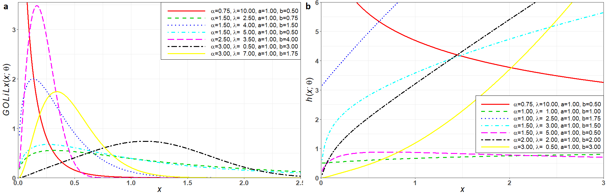
For $b=1$ , we obtain the GOLi-exponential (GOLiE) distribution. For $b=2$ , we obtain the GOLi-Rayleigh (GOLiR) distribution. The GOLiW reduces to the OLiW when $\alpha =1$ . We have the OLiE and OLiR when $\alpha =b=1$ and $\alpha =b=1$ , respectively. Some possible shapes of the GOLiW density and hazard functions are displayed in Figure 1.

Figure 1
Plots of the GOLiW pdf (a) and hrf (b) for some parameter values.

THE GOLi-BURR XII (GOLiBXII) DISTRIBUTION

The cdf (for $x>0$ ) of the Burr XII (BXII) distribution with positive parameters $a$ and $b$ is $G(x)=1-{(1+x^a)}^{-b}$ . Then, the GOLiBXII density reduces to

$\begin{array}{ccc}\hfill f(x)& =\hfill & \hfill \frac{\alpha ab{\lambda }^2}{1+\lambda }{x}^{a-1}{(1+x^a)}^{-b-1}{\{1-{[1-{(1+x^a)}^{-b}]}^{\alpha }\}}^{-3}\\ \hfill & \hfill & \hfill \times {[1-{(1+x^a)}^{-b}]}^{\alpha -1}exp\left\{\frac{-\lambda {[1-{(1+x^a)}^{-b}]}^{\alpha }}{1-{[1-{(1+x^a)}^{-b}]}^{\alpha }}\right\}.\end{array}$

For $a=1$ and $b=1$ , we obtain the one-parameter GOLi Lomax (GOLiLx) and one-parameter GOLi log-logistic (GOLiLL) distributions, respectively. The cases $\alpha =a=1$ and $\alpha =b=1$ refer to the OLiLx and OLiLL distributions, respectively. Plots of the density and hazard functions of the GOLiBXII distribution are displayed in Figure 2.

Figure 2
Plots of the GOLiBXII pdf (a) and hrf (b) for some parameter values.

The GOLi-Lomax (GOLiLx) distribution

The cdf (for $x>0$ ) of the Lomax (Lx) distribution with positive parameters $a$ and $b$ is $G(x)=1-[1+(x/a){]}^{-b}$ . Then, the GOLiLx pdf becomes

$\begin{array}{ccc}\hfill f(x)& =\hfill & \hfill \frac{\alpha b{a}^{-1}{\lambda }^2}{(1+\lambda )}{[1+\left(\frac{x}{a}\right)]}^{-b-1}{(1-{\{1-{[1+\left(\frac{x}{a}\right)]}^{-b}\}}^{\alpha })}^{-3}\\ \hfill & \hfill & \hfill \times {\{1-{[1+\left(\frac{x}{a}\right)]}^{-b}\}}^{\alpha -1}exp\left(\frac{-\lambda {\{1-{[1+\left(\frac{x}{a}\right)]}^{-b}\}}^{\alpha }}{1-{\{1-{[1+\left(\frac{x}{a}\right)]}^{-b}\}}^{\alpha }}\right).\end{array}$

Plots of the density and hazard functions of the GOLiLx distribution are displayed in Figure Figure 3.

Figure 3
Plots of the GOLiLx pdf (a) and hrf (b) for some parameter values.

THE GOLi-LOG-LOGISTIC (GOLiLL) DISTRIBUTION

Consider the cdf (for $x>0$ ) $G(x)=1-{[1+{\left(\frac{x}{a}\right)}^b]}^{-1}$ of the log-logistic (LL) distribution with positive parameters $a$ and $b$ . The GOLiLL density is given by

$\begin{array}{ccc}\hfill f(x)& =\hfill & \hfill \frac{\alpha b{\lambda }^2{x}^{b-1}}{(1+\lambda )a^b}{[1+{\left(\frac{x}{a}\right)}^b]}^{-2}{(1-{\{1-{[1+{\left(\frac{x}{a}\right)}^b]}^{-1}\}}^{\alpha })}^{-3}\\ \hfill & \hfill & \hfill \times {\{1-{[1+{\left(\frac{x}{a}\right)}^b]}^{-1}\}}^{\alpha -1}exp\left(\frac{-\lambda {\{1-{[1+{\left(\frac{x}{a}\right)}^b]}^{-1}\}}^{\alpha }}{1-{\{1-{[1+{\left(\frac{x}{a}\right)}^b]}^{-1}\}}^{\alpha }}\right).\end{array}$

Plots of the density and hazard functions for the GOLiLL distribution for selected parameter values are displayed in Figure 4.

Figure 4
Plots of the GOLiLL pdf (a) and hrf (b) for some parameter values.

LINEAR REPRESENTATION

In this section, we provide a useful linear representation for the GOLi-G density. It can be expressed as

$f(x)=\frac{\alpha {\lambda }^{2}g(x)G(x{)}^{\alpha -1}}{(1+\lambda ){[1-G(x{)}^{\alpha }]}^3}exp\left[\frac{-\lambda G(x{)}^{\alpha }}{1-G(x{)}^{\alpha }}\right].$

Using the exponential series, we can write

$f(x)=\frac{\alpha g(x)}{(1+\lambda )}\sum _{j=0}^{\infty }{(-1)}^j{\lambda }^{j+2}G(x{)}^{(j+1)\alpha -1}\underset{A}{\underbrace{{[1-G(x{)}^{\alpha }]}^{-(j+3)}}}.$ (4)

Consider the power series

${(1-z)}^{-q}=\sum _{n=0}^{\infty }\frac{\Gamma (q+n)}{\Gamma \left(q\right)n!}{z}^n,q>0.$ (5)

Applying this series to the quantity $A$ , we obtain

$A=\sum _{k=0}^{\infty }\frac{(j+k+2)!}{k!(j+2)!}G(x{)}^{k\alpha }.$ (6)

Substituting (6) in equation (4), we can write

$f(x)=\frac{\alpha g(x)}{(1+\lambda )}\sum _{j,k=0}^{\infty }\frac{{(-1)}^j{\lambda }^{j+2}(j+k+2)!}{k!(j+2)!}G(x{)}^{(k+j+1)\alpha -1}.$ (7)

Then, the GOLi-G density can be expressed as a linear combination of exponentiated-G (Exp-G) densities

$f(x)=\sum _{j,k=0}^{\infty }{d}_{j,k}{h}_{(k+j+1)\alpha }(x),$ (8)

where

$d_{j,k}=\frac{1}{(1+\lambda )}\sum _{j,k=0}^{\infty }\frac{{(-1)}^j{\lambda }^{j+2}(j+k+2)!}{(k+j+1)k!(j+2)!}$

and $h_{\delta }\left(x\right)=\delta g\left(x\right)G{\left(x\right)}^{\delta -1}$ is the Exp-G density with power parameter $\delta >0$ . Thus, several mathematical properties of the GOLi-G family can be determined from those properties of the Exp-G family. Equation (8) is the main result of this section.

The cdf of the GOLi-G family can also be expressed as a linear combination of Exp-G cdfs. By integrating (8), we have

$F(x)=\sum _{j,k=0}^{\infty }{d}_{j,k}{H}_{(k+j+1)\alpha }(x),$

where $H_{\delta }\left(x\right)$ is the cdf of the Exp-G family with power parameter $\delta$ .

STRUCTURAL PROPERTIES

In this section, we obtain some structural properties of the GOLi-G family including quantile and generating functions, asymptotics, ordinary and incomplete moments, order statistics and entropies.

QUANTILE FUNCTION

Let $Q_G(\cdot )=G^{-1}(\cdot )$ be the quantile function (qf) of the parent G. In this section, we provide two algorithms for simulating the GOLi-G model.

The first algorithm is based on generating random data from the Li distribution using the exponential-gamma mixture.

• Algorithm 1 (Mixture form of the Li distribution)

1. Generate $U_i\sim Uniform(0,1),i=1,\dots ,n;$

2. Generate $V_i\sim Exponential(\lambda ),i=1,\dots ,n;$

3. Generate $W_i\sim Gamma(2,\lambda ),i=1,\dots ,n;$

If $U_i\le \frac{\lambda }{\lambda +1}$ , set $X_i=G^{-1}([\frac{V_i}{1+V_i}{]}^{1/\alpha })$ ;otherwise, set$X_i=G^{-1}([\frac{W_i}{1+W_i}{]}^{1/\alpha })$

The second algorithm is based on generating random data by inverting (1).

• Algorithm 2 (Inverse cdf)

1. Generate $U_i\sim Uniform(0,1),i=1,\dots ,n;$

Set (for $i=1,\dots ,n$ )

$X_i=G^{-1}\left({\left[\frac{\lambda +W_{-1}[-(1-U_i)(\lambda +1)exp(-\lambda -1)]+1}{W_{-1}[-(1-U_i)(\lambda +1)exp(-\lambda -1)]+1}\right]}^{1/\alpha }\right),$ (9)

where $W(x)$ is the negative branch of the Lambert function. The branches of this function are defined by $x=W(x{e}^x),x\in ℂ$ . It is a two-valued function on the interval $[-1/e,0)$ . For $W(x)\le -1$ , the function is denoted $W_{-1}(x)$ and is called the negative branch. For $W(x)>-1$ , the function is called the principal branch of the W function. The Lambert function cannot be expressed in terms of elementary functions.

ASYMPTOTICS

Let $a=inf\{x|G(x)\}>0$ . Then, the asymptotics of equations (1), (2) and (3) when $x\to a$ are given by

$\begin{array}{c}F\left(x\right)\sim \lambda G(x{)}^{\alpha }\text{as}x\to a,\\ f\left(x\right)\sim \alpha \lambda g(x)G(x{)}^{\alpha -1}\text{as}x\to a,\\ \tau \left(x\right)\sim \alpha \lambda g(x)G(x{)}^{\alpha -1}\text{as}x\to a.\end{array}$

The asymptotics of equations (1), (2) and (3) when $x\to \infty$ are given by

$\begin{array}{c}1-F\left(x\right)\sim \frac{\lambda }{\alpha \overline{G}(x)}\exp [-\lambda /\alpha \overline{G}(x)]\text{ as}x\to \mathrm{\infty },\\ f\left(x\right)\sim \frac{{\lambda }^{2}g(x)}{{\alpha }^2(1+\lambda )\overline{G}(x{)}^3}\exp [-\lambda /\alpha \overline{G}(x)]\text{ as}x\to \mathrm{\infty },\\ \tau \left(x\right)\sim \frac{\lambda g(x)}{{\alpha }^2(1+\lambda )\overline{G}(x{)}^2}\text{ as}x\to \mathrm{\infty }.\end{array}$

GENERATING FUNCTION

Here, we obtain the moment generating function (mgf) $M(t)=E(e^{tX})$ of $X$ . Henceforth, let $T_{(k+j+1)\alpha }$ denote the random variable having the Exp-G class with power parameter $(k+j+1)\alpha$ .

We can write from equation (8)

$M(t)=\sum _{j,k=0}^{\infty }{d}_{j,k}{M}_{(k+j+1)\alpha }(t)=\sum _{j,k=0}^{\infty }{d}_{j,k}{\tau }_{k+j}(t),$

where ${\tau }_{k+j}(t)=(k+j+1)\alpha {\int }_0^{1}exp\left[t{Q}_G\left(u\right)\right]u^{(k+j+1)\alpha -1}du$ and $M_{(k+j+1)\alpha }(t)$ is the mgf of $T_{(k+j+1)\alpha }$ . Hence, $M(t)$ can be determined from the Exp-G generating function. If $M_{(k+j+1)\alpha }(t)$ has an explicit expression, $M(t)$ will also have a closed-form. For some baselines such as the exponential, Lomax, normal, gamma, among others, this is possible.

We define the cumulant generating function (cgf) of $X$ by $K(t)=log[M(t)]$ . The saddle–point approximation is of the main applications of the cgf in Statistics and provides highly accurate approximation formulae for the densities of the sum and mean of independent identically distributed (iid) random variables. Let $X_1,\cdots ,X_n$ be iid random variables having common GOLi-G cgf $K(t)$ . We define $S_n={\sum }_{j=1}^n{X}_j$ and obtain $\hat{\lambda }$ from the (usual nonlinear) equation $K^{\prime }(\hat{\lambda })=x/n$ and let $y=[x-n{K}^{\prime }(\lambda )]/\sqrt{n{K}^{\prime \prime }(\lambda )}$ . The density function of ${\overline{X}}_n=S_n/n$ is followed from Daniels’ saddle–point approximation as

$f_{{\overline{X}}_n}(y)\approx {\left\{\frac{n}{2\pi K^{\prime \prime }(\hat{\lambda })}\right\}}^{1/2}exp[n\{K(\hat{\lambda })-\hat{\lambda }y\}].$

MOMENTS

The $r$ th ordinary moment of $X$ , say ${\mu }_r^{\prime }$ , follows from (8) as

${\mu }_r^{\prime }=E\left(X^r\right)=\sum _{j,k=0}^{\infty }{d}_{j,k}E\left(T_{(k+j+1)\alpha }^r\right).$ (10)

The central moment of $X$ are easily obtained from (10).

The cumulants ( ${\chi }_n$ ) of $X$ follow recursively from

${\chi }_n={\mu }_n^{\mathrm{\prime }}-\sum _{r=0}^{n-1}(\genfrac{}{}{0ex}{}{n-1}{r-1}){\chi }_r{\mu }_{n-r}^{\mathrm{\prime }},$

where ${\chi }_1={\mu }_1^{\mathrm{\prime }}{\chi }_2={\mu }_2^{\mathrm{\prime }}-{\mu }_1^{\mathrm{\prime }2},{\chi }_3={\mu }_3^{\mathrm{\prime }}-3{\mu }_2^{\mathrm{\prime }}{\mu }_1^{\mathrm{\prime }}+{\mu }_1^{\mathrm{\prime }3}$ , etc. The measures of skewness and kurtosis can be calculated from the ordinary moments using well-known relationships.

The $s$ th incomplete moment of $X$ , say ${\phi }_s(t)={\int }_{-\infty }^t{x}^{s}f(x)dx$ , can be expressed from (8) as

${\phi }_s\left(t\right)=\sum _{j,k=0}^{\infty }{d}_{j,k}{\int }_{-\infty }^t{x}^s{h}_{(k+j+1)\alpha }\left(x\right)dx=\sum _{j,k=0}^{\infty }{d}_{j,k}{v}_{(k+j+1)\alpha }^{(s)}\left(t\right),$ (11)

where $v_{(k+j+1)\alpha }^{(s)}\left(t\right)=(k+j+1)\alpha {\int }_0^{G\left(t\right)}{Q}_G{\left(u\right)}^s{u}^{(k+j+1)\alpha -1}du$ can be computed numerically from the baseline qf $Q_G(u)$ .

For $s=1$ , we obtain the first incomplete moment ${\phi }_1(t)$ from (11). It can be applied to construct Bonferroni and Lorenz curves defined for a given probability $\pi$ by $B(\pi )={\phi }_1\left(q\right)/(\pi {\mu }_1^{\prime })$ and $L(\pi )={\phi }_1\left(q\right)/{\mu }_1^{\prime }$ , respectively, where ${\mu }_1^{\prime }$ is given by (10) with $r=1$ and $q=Q(\pi )$ is the qf of $X$ at $\pi$ obtained from (9). These curves are very useful in economics, reliability, demography, insurance and medicine.

ORDER STATISTICS

Order statistics make their appearance in many areas of statistical theory and practice. Let $X_1,\cdots ,X_n$ be a random sample from the GOLi-G family. The pdf of $X_{i:n}$ can be written as

$f_{i:n}\left(x\right)=\frac{f\left(x\right)}{\mathrm{\text{B}}(i,n-i+1)}\sum _{j=0}^{n-i}{(-1)}^j\left(\genfrac{}{}{0ex}{}{n-i}{j}\right)F{\left(x\right)}^{j+i-1},$ (12)

where $B(\cdot ,\cdot )$ is the beta function.

Based on equation (1), we can write

$F{\left(x\right)}^{j+i-1}={\{1-[1+\frac{\lambda G(x{)}^{\alpha }}{1-G(x{)}^{\alpha }}]exp\left[\frac{-\lambda G(x{)}^{\alpha }}{1-G(x{)}^{\alpha }}\right]\}}^{j+i-1}.$

After applying the generalized binomial series, we have

$F{\left(x\right)}^{j+i-1}=\sum _{l=0}^{j+i-1}{(-1)}^l\left(\genfrac{}{}{0ex}{}{j+i-1}{l}\right){[1+\frac{\lambda G(x{)}^{\alpha }}{1-G(x{)}^{\alpha }}]}^{l}exp\left[\frac{-\lambda lG(x{)}^{\alpha }}{1-G(x{)}^{\alpha }}\right].$ (13)

Using (2) and (13), we can write

$\begin{array}{ccc}\hfill f\left(x\right)F{\left(x\right)}^{j+i-1}& =\hfill & \hfill \frac{\alpha {\lambda }^{2}g(x)G(x{)}^{\alpha -1}}{(1+\lambda ){[1-G(x{)}^{\alpha }]}^3}\sum _{l=0}^{j+i-1}{(-1)}^l\left(\genfrac{}{}{0ex}{}{j+i-1}{l}\right)\\ \hfill & \hfill & \hfill \times {[1+\frac{\lambda G(x{)}^{\alpha }}{1-G(x{)}^{\alpha }}]}^{l}exp\left[\frac{-\lambda (l+1)G(x{)}^{\alpha }}{1-G(x{)}^{\alpha }}\right].\end{array}$

Using the exponential series, we obtain

$\begin{array}{ccc}\hfill f\left(x\right)F{\left(x\right)}^{j+i-1}& =\hfill & \hfill \frac{\alpha {\lambda }^{2}g(x)}{(1+\lambda )}\sum _{l=0}^{j+i-1}\sum _{s=0}^{\infty }{(-1)}^{l+s}\left(\genfrac{}{}{0ex}{}{j+i-1}{l}\right)\frac{{\left[\lambda (l+1)\right]}^s}{{[1-G(x{)}^{\alpha }]}^{s+3}}\\ \hfill & \hfill & \hfill \times {[1+\frac{\lambda G(x{)}^{\alpha }}{1-G(x{)}^{\alpha }}]}^{l}G(x{)}^{(s+1)\alpha -1}.\end{array}$

The Taylor series for $z^{\beta }$ defined by

$z^{\beta }=\sum _{k=0}^{\infty }\frac{{\left(\beta \right)}_k}{k!}{(z-1)}^k,$ (14)

holds, where $(\beta {)}_k=\beta (\beta -1)\dots (\beta -k+1)$ is the descending factorial.

Applying (14) to ${[1+\frac{\lambda G(x{)}^{\alpha }}{1-G(x{)}^{\alpha }}]}^l$ gives

${[1+\frac{\lambda G(x{)}^{\alpha }}{1-G(x{)}^{\alpha }}]}^l=\sum _{h=0}^{\infty }{\left(l\right)}_h\frac{{\lambda }^{h}G(x{)}^{h\alpha }}{h!{[1-G(x{)}^{\alpha }]}^h}.$

Then, the last equation reduces to

$\begin{array}{ccc}\hfill f\left(x\right)F{\left(x\right)}^{j+i-1}& =\hfill & \hfill \sum _{l=0}^{j+i-1}\sum _{s,h=0}^{\infty }\frac{{(-1)}^{l+s}{\lambda }^{s+h+2}{(l+1)}^s}{(1+\lambda )h!}{\left(l\right)}_h\left(\genfrac{}{}{0ex}{}{j+i-1}{l}\right)\\ \hfill & \hfill & \hfill \times \frac{\alpha g(x)G(x{)}^{(s+h+1)\alpha -1}}{{[1-G(x{)}^{\alpha }]}^{s+h+3}}.\end{array}$

Applying the power series (5) to ${[1-G(x{)}^{\alpha }]}^{-(s+h+3)}$ gives

$\begin{array}{ccc}\hfill f\left(x\right)F{\left(x\right)}^{j+i-1}& =\hfill & \hfill \sum _{l=0}^{j+i-1}\sum _{s,h,k=0}^{\infty }\frac{{(-1)}^{l+s}{\lambda }^{s+h+2}(s+h+k+2)!}{(1+\lambda ){(l+1)}^{-s}h!k!(s+h+2)!}\\ \hfill & \hfill & \hfill \times {\left(l\right)}_h\left(\genfrac{}{}{0ex}{}{j+i-1}{l}\right)\alpha g(x)G(x{)}^{(k+s+h+1)\alpha -1}.\end{array}$

Inserting the last equation in (12), the pdf of $X_{i:n}$ can be expressed as

$f_{i:n}\left(x\right)=\sum _{s,h,k=0}^{\infty }{m}_{s,h,k}{h}_{(k+s+h+1)\alpha }\left(x\right),$ (15)

where, as before, $h_{\delta }\left(x\right)$ is the Exp-G density with power parameter $\delta$ and

$\begin{array}{ccc}\hfill m_{s,h,k}& =\hfill & \hfill \sum _{j=0}^{n-i}\sum _{l=0}^{j+i-1}\frac{{(-1)}^{l+s+j}{\lambda }^{s+h+2}{(l+1)}^s(s+h+k+2)!}{(1+\lambda )(k+s+h+1)h!k!(s+h+2)}\\ \hfill & \hfill & \hfill \times \frac{{\left(l\right)}_h}{\mathrm{\text{B}}(i,n-i+1)}\left(\genfrac{}{}{0ex}{}{n-i}{j}\right)\left(\genfrac{}{}{0ex}{}{j+i-1}{l}\right).\end{array}$

Then, the density function of the GOLi-G order statistics is a linear combination of Exp-G densities. Based on equation (15), we note that the mathematical properties of $X_{i:n}$ follow from those of $T_{(k+s+h+1)\alpha }$ . For example, the $q$ th moment of $X_{i:n}$ is given by

$E\left(X_{i:n}^q\right)=\sum _{s,h,k=0}^{\infty }{m}_{s,h,k}E\left(T_{(k+s+h+1)\alpha }^q\right).$ (16)

Based upon the moments in equation (16), we can derive explicit expressions for the L-moments of $X$ as infinite weighted linear combinations of the means of suitable GOLi-G order statistics.

ENTROPIES

The Rényi entropy of a random variable $X$ represents a measure of variation of the uncertainty. The Rényi entropy is given by

$I_{\theta }\left(X\right)={(1-\theta )}^{-1}log\left({\int }_{-\infty }^{\infty }f{\left(x\right)}^{\theta }dx\right),\theta >0\mathrm{\text{and}}\theta \ne 1.$

Using the pdf (2), we can write

$f{\left(x\right)}^{\theta }={\left(\frac{\alpha {\lambda }^2}{1+\lambda }\right)}^{\theta }\frac{g(x{)}^{\theta }G(x{)}^{\theta (\alpha -1)}}{{[1-G(x{)}^{\alpha }]}^{3\theta }}exp\left[\frac{-\lambda \theta G(x{)}^{\alpha }}{1-G(x{)}^{\alpha }}\right].$

Using the exponential series, we have

$f{\left(x\right)}^{\theta }={\left(\frac{\alpha {\lambda }^2}{1+\lambda }\right)}^{\theta }g(x{)}^{\theta }\sum _{j=0}^{\infty }{(-1)}^j{\left(\lambda \theta \right)}^{j}G(x{)}^{(\theta +j)\alpha -\theta }{[1-G(x{)}^{\alpha }]}^{-(3\theta +j)}.$

Applying the power series (5) to the last term, we have

$f{\left(x\right)}^{\theta }={\left(\frac{\alpha {\lambda }^2}{1+\lambda }\right)}^{\theta }\sum _{j,k=0}^{\infty }\frac{{(-1)}^j\Gamma (3\theta +j+k)}{k!{\left(\lambda \theta \right)}^{-j}\Gamma (3\theta +j)}g(x{)}^{\theta }G(x{)}^{(k+j+\theta )\alpha -\theta }.$

Then, the Rényi entropy of the GOLi-G family reduces to

$I_{\theta }\left(X\right)={(1-\theta )}^{-1}log[\sum _{j,k=0}^{\infty }{b}_{j,k}{\int }_{-\infty }^{\infty }g(x{)}^{\theta }G(x{)}^{(k+j+\theta )\alpha -\theta }dx],$

where

$b_{j,k}={\left(\frac{\alpha {\lambda }^2}{1+\lambda }\right)}^{\theta }\frac{{(-1)}^j\Gamma (3\theta +j+k)}{k!{\left(\lambda \theta \right)}^{-j}\Gamma (3\theta +j)}.$

The Shannon entropy of $X$ , say $SI=E\{-[logf(X)]\}$ , is given by

$\begin{array}{ccc}\hfill SI& =\hfill & \hfill -log\left(\frac{\alpha {\lambda }^2}{1+\lambda }\right)-E\{log[g(X)]\}+(1-\alpha )E\{log[G(X)]\}\\ \hfill & \hfill & \hfill +3E\{log[1-G(X{)}^{\alpha }]\}+\lambda E\{G(X{)}^{\alpha }/[1-G(X{)}^{\alpha }]\}.\end{array}$

First, we define and compute

$A(a_1,a_2;\alpha ,\lambda )={\int }_0^1\frac{u^{a_1}}{{(1-u^{\alpha })}^{a_2}}exp\left(\frac{-\lambda u^{\alpha }}{1-u^{\alpha }}\right)du.$

By using the exponential series, we obtain

$A(a_1,a_2;\alpha ,\lambda )=\sum _{i=0}^{\infty }\frac{{(-1)}^i}{i!}{\lambda }^i{\int }_0^1\frac{u^{a_1+\alpha i}}{{(1-u^{\alpha })}^{a_2+i}}du.$

Using the binomial expansion, we have

$A(a_1,a_2;\alpha ,\lambda )=\sum _{i,j=0}^{\infty }\frac{{(-1)}^{i+j}{\lambda }^i}{i![a_1+\alpha (j+i)]}\left(\genfrac{}{}{0ex}{}{-a_2-i}{j}\right).$

The following proposition is used to determine the Shannon entropy of $X$ .Proposition 1. Let $X$ be a random variable with pdf given in (2). Then,

$\begin{array}{ccc}\hfill E\{log[G(X)]\}& =\hfill & \hfill \frac{\alpha {\lambda }^2}{1+\lambda }\frac{\partial }{\partial t}A(\alpha +t-1,3;\alpha ,\lambda ){|}_{t=0},\\ \hfill E\{log[1-G(X{)}^{\alpha }]\}& =\hfill & \hfill \frac{\alpha {\lambda }^2}{1+\lambda }\frac{\partial }{\partial t}A(\alpha -1,-t+3;\alpha ,\lambda ){|}_{t=0}\mathrm{\text{and}}\\ \hfill E\{G(X{)}^{\alpha }/[1-G(X{)}^{\alpha }]\}& =\hfill & \hfill \frac{\alpha {\lambda }^2}{1+\lambda }A(2\alpha -1,4;\alpha ,\lambda ).\end{array}$

MAXIMUM LIKELIHOOD ESTIMATION

Several approaches for parameter estimation were proposed in the literature but the maximum likelihood method is the most commonly employed. The maximum likelihood estimators (MLEs) enjoy desirable properties and can be used to obtain confidence intervals for the model parameters. The normal approximation for these estimators in large samples can be easily handled either analytically or numerically. Here, we consider the estimation of the unknown parameters of the new family from complete samples only by maximum likelihood.

Let $X_1,\cdots ,X_n$ be a random sample from the GOLi-G family with parameters α,λ and $𝛗$ . Let $𝛉=$ ( $\alpha ,\lambda ,{𝛗}^{⊺}$ ) ${}^{⊺}$ be the $p\times 1$ parameter vector. The log-likelihood function for $𝛉$ is given by

$\begin{array}{ccc}\hfill \ell (𝛉)& =\hfill & \hfill nlog\left(\alpha \right)+2nlog\left(\lambda \right)-nlog(1+\lambda )+(\alpha -1)\sum _{i=1}^{n}logG(x_i;𝛗)\\ \hfill & \hfill & \hfill +\sum _{i=1}^{n}logg(x_i;𝛗)-3\sum _{i=1}^{n}log[1-G(x_i;𝛗{)}^{\alpha }]-\lambda \sum _{i=1}^n\frac{G(x_i;𝛗{)}^{\alpha }}{1-G(x_i;𝛗{)}^{\alpha }}.\end{array}$

Then, the score vector components, $𝐔\left(𝛉\right)=\frac{\partial \ell }{\partial 𝛉}={(U_{\alpha },U_{\lambda },U_{{\phi }_k})}^{⊺}$ , are

$\begin{array}{ccc}\hfill U_{\alpha }& =\hfill & \hfill \frac{n}{\alpha }+\sum _{i=1}^{n}logG(x_i;𝛗)+3\sum _{i=1}^n\frac{G(x_i;𝛗{)}^{\alpha }logG(x_i;𝛗)}{1-G(x_i;𝛗{)}^{\alpha }}\\ \hfill & \hfill & \hfill -\lambda \sum _{i=1}^n\frac{G(x_i;𝛗{)}^{\alpha }logG(x_i;𝛗)}{{[1-G(x_i;𝛗{)}^{\alpha }]}^2},\end{array}$

$U_{\lambda }=\frac{2n}{\lambda }-\frac{n}{1+\lambda }-\sum _{i=1}^n\frac{G(x_i;𝛗{)}^{\alpha }}{1-G(x_i;𝛗{)}^{\alpha }}$

and

$\begin{array}{ccc}\hfill U_{{\phi }_k}& =\hfill & \hfill \sum _{i=1}^n\frac{g_k^{\prime }(x_i;𝛗)}{g(x_i;𝛗)}+(\alpha -1)\sum _{i=1}^n\frac{G_k^{\prime }(x_i;𝛗)}{G(x_i;𝛗)}+3\alpha \sum _{i=1}^n\frac{G_k^{\prime }(x_i;𝛗{)}^{\alpha -1}}{1-G(x_i;𝛗{)}^{\alpha }}\\ \hfill & \hfill & \hfill -\lambda \alpha \sum _{i=1}^n\frac{G_k^{\prime }(x_i;𝛗{)}^{\alpha -1}}{{[1-G(x_i;𝛗{)}^{\alpha }]}^2},\end{array}$

where $g_k^{\prime }(x_i;𝛗)=\partial g(x_i;𝛗)/\partial {\phi }_k$ and $G_k^{\prime }(x_i;𝛗)=\partial G(x_i;𝛗)/\partial {\phi }_k.$

Setting the nonlinear system of equations $U_{\alpha }=U_{\lambda }=0$ and $U_{𝛗}=0$ and solving them simultaneously yields the MLE $\widehat{𝛉}=(\hat{\alpha },\hat{\lambda },{\widehat{𝛗}}^{⊺}{)}^{⊺}$ . For doing this, it is usually more convenient to adopt nonlinear optimization methods such as the quasi-Newton algorithm to maximize $\ell$ numerically. For interval estimation of the parameters, we obtain the $p\times p$ observed information matrix $J(𝛉)=\{-\frac{{\partial }^2\ell }{\partial r\partial s}\}$ (for $r,s=\alpha ,\lambda ,{\phi }_k$ ), which can be evaluated numerically.

Under standard regularity conditions, the distribution of $\widehat{𝛉}$ can be approximated by a multivariate normal $N_p(0,J(\widehat{𝛉}{)}^{-1})$ distribution when $n\to \infty$ to obtain confidence intervals for the parameters. Here, $J(\widehat{𝛉})$ is the total observed information matrix evaluated at $\widehat{𝛉}$ . The method of the re-sampling bootstrap can be used for correcting the biases of the MLEs of the model parameters. Good interval estimates may also be obtained using the bootstrap percentile method.

SIMULATION STUDY

In this section, we present some simulation results that investigate the behavior of the MLEs in terms of the sample size $n$ . All simulations are performed using the Rprogramming language (R Core Team 2017).

The qf of the GOLiW distribution is given by

$Q(p)={(-\frac{1}{a}log\{1-{\left[\frac{\lambda +W_{-1}[(p-1)(\lambda +1)exp(-\lambda -1)]+1}{W_{-1}[(p-1)(\lambda +1)exp(-\lambda -1)]+1}\right]}^{\frac{1}{\alpha }}\})}^{\frac{1}{b}}.$

We generate $2,000$ random samples from this distribution using the last expression for three different sample sizes $n=350$ , $n=550$ and $n=750$ . The true values of the parameters are taken as: $\alpha =(0.2,1,2),\lambda =(0.5,2),a=(0.7,2.5,4.3)$ and $b=(0.9,3,5)$ . For each sample size and parameter combination, the average MLEs and the mean square errors (MSEs) are computed. In order to save space, Table I gives only the results for $\alpha =2$ , and are not reported for $\alpha =(0.2,1)$ . It can be verified that the estimates are stable and quite close the true parameter values for all sample sizes. Further, the MSEs decrease when the sample size increases in all cases in agreement with the first-order asymptotic theory.

TABLE I
Average values of the MLEs and the corresponding MSEs for α = 2 and (n=350, 550 and 750).

n	$\hat{\alpha }$	$MSE(\hat{\alpha })$	λ	$\hat{\lambda }$	$\text{MSE}(\hat{\lambda })$	a	$\hat{a}$	$\text{MSE}(\hat{a})$	b	$\hat{b}$	$\text{MSE}(\hat{b})$
350	2.47785	3.57641	0.5	0.50116	0.00037	0.7	0.76066	0.12152	0.9	0.91553	0.03548
550	2.26562	1.43760		0.50075	0.00026		0.73673	0.07164		0.90973	0.02123
750	2.19027	0.82444		0.49994	0.00018		0.72749	0.05207		0.90729	0.01567
350	2.48698	3.04369		0.50097	0.00037		0.76611	0.12216	3.0	3.04001	0.38174
550	2.35512	1.77756		0.50053	0.00024		0.75840	0.07948		2.99564	0.23581
750	2.18049	0.77913		0.50048	0.00018		0.72470	0.05077		3.02977	0.17295
350	2.56685	3.99778		0.50171	0.00039		0.78214	0.13450	5.0	5.02180	1.10152
550	2.29636	1.34325		0.50041	0.00023		0.74661	0.07026		5.01681	0.61638
750	2.22297	0.79798		0.50049	0.00017		0.73822	0.05116		5.00113	0.45527
350	2.52108	4.49541		0.50067	0.00040	2.5	2.57087	0.27583	0.9	0.91488	0.03812
550	2.28265	1.34818		0.50071	0.00024		2.54553	0.15601		0.90647	0.02071
750	2.16575	0.69721		0.50030	0.00018		2.52146	0.10832		0.90822	0.01519
350	2.60060	5.04284		0.50075	0.00038		2.59315	0.28616	3.0	3.01851	0.38213
550	2.32758	2.52439		0.50068	0.00024		2.55328	0.16813		3.01762	0.24144
750	2.18993	0.76092		0.50050	0.00018		2.53138	0.10957		3.01966	0.16518
350	2.49875	4.91899		0.50165	0.00036		2.56453	0.26356	5.0	5.07914	1.03591
550	2.28231	1.38029		0.50047	0.00025		2.54382	0.16013		5.04115	0.65936
750	2.20620	0.74794		0.50006	0.00018		2.53896	0.11032		5.01394	0.45806
350	2.50010	5.20868		0.50130	0.00039	4.3	4.37869	0.18204	0.9	0.91435	0.03498
550	2.27733	1.24864		0.50083	0.00025		4.35394	0.10463		0.90657	0.02101
750	2.18215	0.68739		0.50072	0.00018		4.34226	0.07059		0.90677	0.01501
350	2.63310	4.44811		0.50226	0.00039		4.41352	0.20697	3.0	3.00294	0.38661
550	2.32132	1.64614		0.50071	0.00024		4.36402	0.11117		3.01137	0.23855
750	2.22868	0.84644		0.50041	0.00018		4.35037	0.07886		3.00408	0.16942
350	2.44902	3.50202		0.50017	0.00040		4.37362	0.17580	5.0	5.11283	1.08059
550	2.32181	1.41633		0.50047	0.00024		4.36786	0.11115		5.00644	0.63025
750	2.17571	0.71741		0.50056	0.00018		4.33550	0.07252		5.04160	0.46412
350	2.30486	2.08277	2.0	2.00368	0.00750	0.7	0.74786	0.10516	0.9	0.93034	0.05804
550	2.15112	0.67356		2.00226	0.00470		0.72423	0.05835		0.91879	0.03046
750	2.10368	0.39468		2.00078	0.00340		0.71692	0.04031		0.91497	0.02208
350	2.25492	1.33882		2.00225	0.00723		0.73784	0.09783	3.0	3.12346	0.71101
550	2.13798	0.67363		1.99995	0.00435		0.71945	0.05852		3.07807	0.35595
750	2.11914	0.43386		2.00001	0.00356		0.72139	0.04315		3.04201	0.25828
350	2.28741	1.35652		2.00506	0.00747		0.74795	0.09982	5.0	5.16168	1.75064
550	2.19248	0.73292		2.00276	0.00470		0.73579	0.06384		5.07695	1.01064
750	2.12997	0.44600		2.00306	0.00358		0.72454	0.04370		5.05948	0.70877
350	2.26410	1.52295		2.00196	0.00783	2.5	2.54455	0.11435	0.9	0.93847	0.05952
550	2.17711	0.73567		2.00191	0.00462		2.53418	0.06981		0.91443	0.03068
750	2.10840	0.41262		2.00299	0.00354		2.52255	0.04742		0.91483	0.02286
350	2.27206	1.48501		2.00657	0.00725		2.55000	0.11461	3.0	3.12107	0.63362
550	2.14655	0.63521		2.00258	0.00465		2.52724	0.06762		3.07540	0.36154
750	2.10247	0.43702		2.00069	0.00343		2.51833	0.04785		3.05464	0.25187
350	2.29692	1.57601		2.00340	0.00720		2.55633	0.11672	5.0	5.18189	1.90371
550	2.13263	0.68456		2.00081	0.00445		2.51781	0.06929		5.15111	1.09036
750	2.09321	0.41101		2.00179	0.00340		2.51647	0.04651		5.09579	0.68370
350	2.32903	1.61028		2.00543	0.00762	4.3	4.45296	0.12749	0.9	0.92361	0.05614
550	2.15238	0.66621		2.00276	0.00471		4.38676	0.05886		0.92085	0.03299
750	2.09719	0.39013		2.00076	0.00330		4.35575	0.03260		0.91460	0.02165
350	2.31347	1.50773		2.00079	0.00753		4.44388	0.12973	3.0	3.07847	0.62103
550	2.13992	0.67529		2.00325	0.00451		4.39256	0.06239		3.08653	0.37296
750	2.11888	0.45106		1.99907	0.00336		4.36968	0.03603		3.04865	0.25858
350	2.24846	1.46959		2.00295	0.00746		4.44081	0.12498	5.0	5.19737	1.70506
550	2.15252	0.63939		2.00190	0.00469		4.38198	0.05560		5.11136	1.03083
750	2.07391	0.38562		2.00203	0.00346		4.36451	0.03638		5.12284	0.69942

APPLICATIONS

In this section, we provide two applications to real data to illustrate the flexibility of the GOLiLx, GOLiLL and GOLiBXII distributions presented in Section 2. The goodness-of-fit statistics for these models are compared with other competitive models and the MLEs of the model parameters are determined.

The model selection is carried out using some goodness-of-fit measures including the Akaike information criterion ( $AIC$ ), consistent Akaike information criterion ( $CAIC$ ), Hannan-Quinn information criterion ( $HQIC$ ), Bayesian information criterion ( $BIC$ ), Anderson-Darling $(A^{*})$ and Cramér-von Mises ( $W^{*}$ ). The smaller these statistics are, the better the fit.

APPLICATION 1: TIME-TO-FAILURE OF TURBOCHARGER DATA

The first data set consists of 40 times to failures ( ${10}^3$ h) of turbocharger of one type of engine given in Xu et al. (2003). For these data, we shall compare the fit of the GOLiLx and GOLiLL distributions with those of other competitive models, namely: the Kumaraswamy transmuted log-logistic (KwTLL) (Afify et al. 2016), Kumaraswamy log-logistic (KwLL) (de Santana et al. 2012), transmuted log-logistic (TLL) (Granzotto and Louzada 2015), McDonald log-logistic (McLL) (Tahir et al. 2014), beta log-logistic (BLL) (Lemonte 2014), generalized transmuted log-logistic (GTLL) (Nofal et al. 2017) and Li-log-logistic (LiLL) (Cakmakyapan and Ozel 2016) distributions, whose densities (for $x>0$ ) are given, respectively, by: KwTLL: $f\left(x\right)=ab\beta {\alpha }^{-\beta }{x}^{\beta -1}{[1+{\left(\frac{x}{\alpha }\right)}^{\beta }]}^{-2}{\{1-{[1+{\left(\frac{x}{\alpha }\right)}^{\beta }]}^{-1}\}}^{a-1}$

$\times \{1-\lambda +2\lambda {[1+{\left(\frac{x}{\alpha }\right)}^{\beta }]}^{-1}\}{\{1+\lambda {[1+{\left(\frac{x}{\alpha }\right)}^{\beta }]}^{-1}\}}^{a-1}$

$\times {\{1-{[1+\lambda {[1+{\left(\frac{x}{\alpha }\right)}^{\beta }]}^{-1}]}^a{\{1-{[1+{\left(\frac{x}{\alpha }\right)}^{\beta }]}^{-1}\}}^a\}}^{b-1};$

KwLL: $f(x)=\frac{ab\beta }{{\alpha }^{a\beta }}{x}^{a\beta -1}{[1+{\left(\frac{x}{\alpha }\right)}^{\beta }]}^{-a-1}{\{1-{[1-\frac{1}{1+{\left(\frac{x}{\alpha }\right)}^{\beta }}]}^a\}}^{b-1};$

TLL: $f(x)=\beta {\alpha }^{-\beta }{x}^{\beta -1}{[1+{\left(\frac{x}{\alpha }\right)}^{\beta }]}^{-2}\{1-\lambda +2\lambda {[1+{\left(\frac{x}{\alpha }\right)}^{\beta }]}^{-1}\};$

McLL: $f(x)=\frac{\beta c}{\alpha B(a/c,b)}{\left(\frac{x}{\alpha }\right)}^{\beta a-1}{[1+{\left(\frac{x}{\alpha }\right)}^{\beta }]}^{-a-1}$

$\times {\{1-{[1-{[1+{\left(\frac{x}{\alpha }\right)}^{\beta }]}^{-1}]}^c\}}^{b-1};$

BLL: $f(x)=\frac{\beta {\alpha }^{-a\beta }}{B(a,b)}{x}^{a\beta -1}{[1+{\left(\frac{x}{\alpha }\right)}^{\beta }]}^{-a-b};$

GTLL: $f(x)=\beta {\alpha }^{-\beta }{x}^{\beta -1}{[1+{\left(\frac{x}{\alpha }\right)}^{\beta }]}^{-2}{\{1-{[1+{\left(\frac{x}{\alpha }\right)}^{\beta }]}^{-1}\}}^{a-1}$

$\times \{a(1+\lambda )-\lambda (a+b){\{1-{[1+{\left(\frac{x}{\alpha }\right)}^{\beta }]}^{-1}\}}^b\};$

LiLL: $f(x)=\frac{\beta {\lambda }^2{\alpha }^{-\beta }}{(1+\lambda )}{x}^{\beta -1}{[1+{\left(\frac{x}{\alpha }\right)}^{\beta }]}^{-\lambda -1}(1-log\left\{{[1+{\left(\frac{x}{\alpha }\right)}^{\beta }]}^{-1}\right\}).$ The parameters of the above densities are all positive real numbers except for the KwTLL, TLL and GTLL models for which the parameter $\lambda$ is $\left|\lambda \right|\le 1$ .

APPLICATION 2: CANCER PATIENTS DATA

The second data set on the remission times (in months) of a random sample of 128 bladder cancer patients (Lee and Wang 2003). For these data, we compare the fit of the GOLiBXII distribution with those of the OLiBXII, Weibull BXII (WBXII) (Afify et al. 2018), Kumaraswamy exponentiated Burr XII (KwEBXII) (Mead and Afify 2017), McDonald Weibull (McW) (Cordeiro et al. 2014), beta BXII (BBXII) (Paranaíba et al. 2011), beta exponentiated BXII (BEBXII) (Mead 2014), LiBXII (Cakmakyapan and Ozel 2016) and BXII models with densities (for $x>0$ ), respectively, given by:

WBXII: $f(x)=\alpha \lambda ab{x}^{\alpha -1}{(1+x^{\alpha })}^{\lambda b-1}{[1-{(1+x^{\alpha })}^{-\lambda }]}^{b-1}$

$\times exp\{-a{[{(1+x^{\alpha })}^{\lambda }-1]}^b\};$

KwEBXII: $f(x)=\frac{abck\beta x^{c-1}}{{(1+x^c)}^{k+1}}{[1-{(1+x^c)}^{-k}]}^{a\beta -1}$

$\times {\{1-{[1-{(1+x^c)}^{-k}]}^{a\beta }\}}^{b-1};$

McW: $f(x)=\frac{\beta c{\alpha }^{\beta }}{B(a/c,b)}{x}^{\beta -1}{e}^{-{\left(\alpha x\right)}^{\beta }}{[1-e^{-{\left(\alpha x\right)}^{\beta }}]}^{a-1}$

$\times {\{1-{[1-e^{-{\left(\alpha x\right)}^{\beta }}]}^c\}}^{b-1};$

BBXII: $f(x)=\frac{c\theta {\beta }^{-c}}{B(a,b)}{x}^{c-1}{[1+{\left(\frac{x}{\beta }\right)}^c]}^{-\theta b-1}{\{1-{[1+{\left(\frac{x}{\beta }\right)}^c]}^{-\theta }\}}^{a-1};$

BEBXII: $f(x)=\frac{c\theta \beta }{B(a,b)}{x}^{c-1}{(1+x^c)}^{-\theta -1}{[1-{(1+x^c)}^{-\theta }]}^{a\beta -1}$

$\times {\{1-{[1-{(1+x^c)}^{-\theta }]}^{\beta }\}}^{b-1};$

LiBXII: $f(x)=\frac{ab{\lambda }^2}{(1+\lambda )}{x}^{a-1}{(1+x^a)}^{-b\lambda -1}\{1-log\left[{(1+x^a)}^{-b}\right]\}.$ All the above parameters are positive real numbers.

Tables II and IV list the values of $AIC$ , $CAIC$ , $HQIC$ , $BIC$ , $W^{*}$ and $A^{*}$ , whereas the MLEs and their corresponding standard errors (in parentheses) of the model parameters are given in Tables III and V.

TABLE II
Goodness-of-fit statistics for time-to-failure data.

Model	AIC	CAIC	HQIC	BIC	W*	A*
GOLiLx	175.045	176.187	177.487	181.800	0.1020	0.7305
GOLiLL	175.945	177.078	178.387	182.700	0.1173	0.8197
KwTLL	184.116	185.880	187.169	192.560	0.2029	1.3256
KwLL	182.470	183.613	184.913	189.226	0.2072	1.3504
TLL	$183.413$	$184.080$	$185.245$	$188.480$	$0.2161$	$1.3995$
McLL	$190.374$	$192.139$	$193.428$	$198.819$	$0.2895$	$1.8181$
BLL	$189.769$	$190.912$	$192.212$	$196.525$	$0.3068$	$1.9212$
GTLL	$211.936$	$213.701$	$214.990$	$220.381$	$0.5591$	$3.3694$
LiLL	$228.936$	$229.602$	$230.768$	$234.002$	$0.7117$	$4.4281$

TABLE III
MLEs and their standard errors (in parentheses) for time-to-failure data.

Model	$\lambda$	$\alpha$	$\beta$
TLL	0.0007	6.2257	4.8416
	(0.8200)	(0.9951)	(0.6540)
LiLL	0.0557	1.6560	27.6744
	(0.0220)	(0.0570)	(9.4810)
	$\alpha$	$\lambda$	$a$	$b$
GOLiLx	73.8241	0.0692	0.4833	2.8316
	(0.0009)	(0.0500)	(1.7480 x 106)	(0.2650)
GOLiLL	35.4255	0.0670	0.4230	2.5184
	(0.0011)	(0.0490)	(5.0250 x 106)	(0.2580)
	$\alpha$	$\beta$	$a$	$b$
KwLL	0.5882	0.7449	28.9123	77.0219
	(0.8820)	(0.1010)	(25.7920)	(61.3480)
BLL	4.9462	0.7316	25.3193	22.3871
	(1.2120)	(0.1210)	(18.7250)	(14.3040)
	$\alpha$	$\beta$	$a$	$b$	λ
KwTLL	0.1739	0.6619	56.2427	118.6118	0.0006
	(0.1300)	(0.1060)	(44.7200)	(100.2550)	(1.4020)
GTLL	0.8271	2.0222	34.4721	0.7329	4.2209 x 106
	(0.409)	(0.2030)	(31.1840)	(18.7070)	(0.0460)
	$\alpha$	$\beta$	$a$	$b$	$c$
McLL	17.3407	0.6128	32.4696	49.3263	0.6020
	(0.2880)	(19.9640)	(28.4240)	(10.0180)	(1.4040)

TABLE IV
Goodness-of-fit statistics for cancer data.

Model	AIC	CAIC	HQIC	BIC	W*	A*
GOLiBXII	829.713	830.038	834.348	841.121	0.04336	0.28618
WBXII	829.812	830.138	834.448	841.221	0.04976	0.32650
KwEBXII	831.651	832.143	837.445	845.911	0.04817	0.31966
McW	831.680	832.172	837.474	845.940	0.05037	0.32985
BBXII	832.297	832.789	838.091	846.557	0.04116	0.29716
OLiBXII	832.793	832.987	836.270	841.350	0.11701	0.70190
BEBXII	841.268	841.760	847.062	855.528	0.13369	0.90004
LiBXII	868.200	868.394	871.677	876.756	0.37270	2.71926
BXII	910.950	911.046	913.267	916.654	0.69396	5.37094

TABLE V
MLEs and their standard errors (in parentheses) for cancer data.

Model	a	b
BXII	2.3354	0.2337
	(0.3540)	(0.0400)
	$\lambda$	a	b
OLiBXII	0.2810	0.8766	0.9669
	(0.1640)	(0.5520)	(0.7690)
LiBXII	0.0472	1.7448	12.7645
	(0.2880)	(14.0960)	(0.0470)
	$\alpha$	$\lambda$	a	b
GOLiBXII	0.7684	0.4170	1.7800	0.3712
	(0.0013)	(0.0760)	(0.0037)	(0.0340)
WBXII	0.7890	0.2008	6.7391	2.4552
	(0.4018)	(0.3120)	(43.9190)
	$\alpha$	$\beta$	$a$	b	$c$
McW	0.1192	0.5582	4.0633	2.6036	0.0393
	(0.1090)	(0.1780)	(2.1110)	(2.4520)	(0.2020)
	$\theta$	$\beta$	$a$	b	c
KwEBXII	0.8389	3.0825	2.7800	67.6361	0.3383
	(1.7230)	(49.3530)	(44.5100)	(104.7280)	(0.3850)
BBXII	0.8665	6.3741	1.0891	1.3905	1.5728
	(1.0170)	(1.5820)	(0.4510)	(2.4050)	(0.4410)
BEBXII	1.3064	1.7799	22.1864	20.2769	0.2245
	(1.0790)	(1.0760)	(21.9560)	(17.2960)	(0.1440)

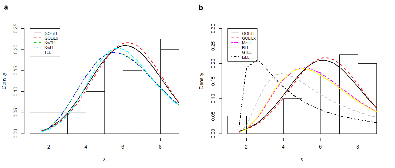
The fitted GOLiLL and GOLiLx pdfs and other fitted pdfs for the time-to-failure data are displayed in Figure 5, whereas the PP-plots of these fitted models are displayed in ^{Figure S7 (Supplementary Material)}. These plots reveal that the GOLiLx and GOLiLL distributions provide the best fits and can be considered very competitive models to other non-nested distributions.

Figure 5
The estimated GOLiLL and GOLiLx pdfs and other estimated pdfs for time-to-failure data. (a) The estimated GOLiLL, GOLiLx, KwTLL, KwLL and TLL densities. (b) The estimated GOLiLL, GOLiLx, McLL, BLL, GTLL and LiLL densities.

The plots of the fitted GOLiBXII pdf and other fitted pdfs defined before, for the cancer data, are displayed in Figure 6. The PP-plots of the fitted models are given in Figure S8. These plots reveal that the GOLiBXII distribution provides the best fits and it can be considered a very competitive model to other distributions with positive support.

Figure 6
The estimated GOLiBXII pdf and other estimated pdfs for cancer data. (a) The estimated GOLiBXII, WBXII, KwEBXII, McW and LiBXII densities. (b) The estimated GOLiBXII, BBXII, OLiBXII, BEBXII and BXII densities.

CONCLUSIONS

In this paper, we propose a new family of distributions with two extra positive parameters called the generalized odd Lindley-G family. The new family extends several widely known distributions and four of its special models are discussed. We demonstrate that its density function is a linear combination of exponentiated-G densities. We obtain some mathematical properties of the new family, which include quantile and generating functions, asymptotics, ordinary and incomplete moments, order statistics and entropies. The model parameters are estimated by the methods of maximum likelihood. Simulation results are reported for this method. Two real examples are used for illustration, where the new family does fit well both data sets.

REFERENCES

• AFIFY AZ, CORDEIRO GM, ORTEGA EMM, YOUSOF HM and BUTT NS. 2018. The four-parameter Burr XII distributions: properties, regression model and applications. Commun Stat - Theory Methods 47: 2605-2624.
• AFIFY AZ, CORDEIRO GM, YOUSOF HM, ALZAATREH A and NOFAL ZM. 2016. The Kumaraswamy transmuted-G family of distributions: properties and applications. Journal of Data Science 14: 245-270.
• ALZAATREH A, LEE C and FAMOYE F. 2013. A new method for generating families of distributions. Metron 71: 63-79.
• BAKOUCH HS, AL-ZAHRANI BM, AL-SHOMRANI AA, MARCHI VAA and LOUZADA F. 2012. An extended Lindley distribution. J Korean Stat Soc 41: 75-85.
• CAKMAKYAPAN S and OZEL G. 2016. The Lindley family of distributions: properties and applications. Hacet J Math Stat 46: 1-27.
• DE SANTANA TVF, ORTEGA EMM, CORDEIRO GM and SILVA GO. 2012. The Kumaraswamy log-logistic distribution. Stat Theory Appl 3: 265-291.
• GHITANY ME, AL-MUTAIRI DK, BALAKRISHNAN N and AL-ENEZI L. 2013. Power Lindley distribution and associated inference. Comput Stat Data Anal 64: 20-33.
• GHITANY M, ATIEH B and NADARAJAH S. 2008. Lindley distribution and its application. Math Comp Simul 78: 493-506.
• GOMES-SILVA FS, PERCONTINI A, BRITO E, RAMOS MW, VENÂNCIO R and CORDEIRO GM. 2017. The Odd Lindley-G Family of Distributions. Austrian Journal of Statistics 46: 65-87.
• GRANZOTTO DCT and LOUZADA F. 2015. The transmuted log-logistic distribution: modeling, inference and na application to a polled tabapua race time up to first calving data. Commun Stat - Theory Methods 44: 3387-3402.
• HUSSAIN E. 2006. The non-linear functions of order statistics and their properties in selected probability models. Ph.D. thesis. Department of Statistics. University of Karachi, Pakistan.
• LEE ET and WANG JW. 2003. Statistical methods for survival data analysis. 3rd ed., Wiley, New York.
• LEMONTE AJ. 2014. The beta log-logistic distribution. Braz J Probab Stat 28: 313-332.
• LINDLEY DV. 1958. Fiducial distributions and Bayes’ theorem. J R Stat Soc Series B 20: 102-107.
• MAHMOUDI E and ZAKERZADEH H. 2010. Generalized Poisson–Lindley distribution. Commun Stat - Theory Methods 39: 1785-1798.
• MEAD ME. 2014. The beta exponentiated Burr XII distribution. Journal of Statistics: Advances in Theory and Applications 12: 53-73.
• MEAD ME and AFIFY AZ. 2017. On five-parameter Burr XII distribution: properties and applications. South African Statistical Journal 51: 67-80.
• NADARAJAH S, BAKOUCH HS and TAHMASBI R. 2011. A generalized Lindley distribution. Sankhya B 73: 331-359.
• NEDJAR S and ZEGHDOUDI H. 2016. Gamma Lindley distribution and its application. J Appl Probab Stat 11: 129-138.
• NOFAL ZM, AFIFY AZ, YOUSOF HM and CORDEIRO GM. 2017. The generalized transmuted-G family of distributions. Commun Stat - Theory Methods 46: 4119-4136.
• PARANAÍBA PF, ORTEGA EMM, CORDEIRO GM and PESCIM RR. 2011. The beta Burr XII distribution with application to lifetime data. Comput Stat Data Anal 55: 1118-1136.
• R CORE TEAM. 2017. R: A language and environment for statistical computing. R Foundation for Statistical Computing.
• SANKARAN M. 1970. The discrete Poisson–Lindley distribution. Biometrics 26: 145-149.
• TAHIR MH, MANSOOR M, ZUBAIR M and HAMEDANI G. 2014. McDonald log-logistic distribution with an application to breast cancer data. Journal of Statistical Theory and Applications 13: 65-82.
• XU K, XIE M, TANG LC and HO SL. 2003. Application of neural networks in forecasting engine systems reliability. Appl Soft Comput 2: 255-268.
• ZAKERZADEH H and DOLATI A. 2009. Generalized Lindley Distribution. J Math Ext 3: 13-25.
• ZAMANI H and ISMAIL N. 2010. Negative binomial-Lindley distribution and its application. Journal of Mathematics and Statistics 6: 4-9.

Publication Dates

• Publication in this collection
  12 Aug 2019
• Date of issue
  2019

History

• Received
  12 Jan 2018
• Accepted
  13 Nov 2018