Inference of leaf nitrogen concentration using machine learning on data resampled to the spectral resolution of Sentinel-2

ABSTRACT.

Nitrogen (N) is among the main nutrients widely used in agriculture worldwide; however, its administration and management can be challenging. Excess nitrogen is harmful to plant health and the environment, requiring effective monitoring of leaf nitrogen concentration (LNC) in field crops. Remote sensing stands out as a valuable tool in this context. This study contributed to the monitoring of LNC by implementing a machine learning algorithm based on the processing of reflectance data from Sentinel-2 (S2) satellites obtained via spectral resampling. For this purpose, five independent datasets containing leaf reflectance measurements collected by spectroradiometers were resampled to the spectral resolution of the sensors onboard the S2 satellites. LNC prediction models were developed from the resampled datasets, using Support Vector Regression (SVR) and Random Forest Regression (RFR), with 75% of the data from each set used to train a model and the remaining 25% for validation. The models demonstrated good predictive power, with the Root Mean Squared Error (RMSE) ranging from 0.39 to 0.94%. Furthermore, this study investigated the transferability of the models' predictive power by using 100% of the data from each set for training and validating predictions on the other sets. To improve transferability, the Transfer Component Analysis (TCA) technique was applied to adapt domains between the sets. This analysis revealed favorable results, especially with the TCA-SVR and TCA-RFR combinations, highlighting a greater capacity to extract transferable spectral features between different leaf reflectance datasets. It was concluded that spectral resampling does not hinder the development of effective LNC prediction models. Aligning this resampling with the resolution of Sentinel-2 sensors, resulted in more efficient monitoring of LNC, eliminating the need to individually reference each sampling point. This approach simplified the monitoring process, reduced both time and costs, and was directly beneficial to producers.

Keywords:
remote sensing; reflectance data; transferability of predictive power; support vector regression; random forest regression; transfer component analysis

Introduction

Nitrogen (N) is a key nutrient in global agriculture, essential for plant growth and productivity. However, it is easily lost in production systems because of its high reactivity, thereby complicating its management. To prevent nutrient deficiencies, farmers often excessively apply nitrogen, which can cause adverse effects. According to Cilia et al. (2014), the unabsorbed fraction of nitrogen can cause nutritional imbalances in plants and environmental issues such as leaching and greenhouse gas emissions.

Consequently, farmers have traditionally relied on methods of chemical laboratory analysis of the tissue, known as foliar diagnosis, to determine the foliar content of the nutrient and estimate the correct nitrogen fertilizer dosage, ensuring that the plant's nutritional demands are met for optimal production. Ideally, these analyses should be conducted periodically throughout the year, which imposes time and costs on producers (Muñoz-Huerta et al., 2013).

Indeed, an efficient method for large-scale monitoring of N in the field is only possible through remote sensing (Berger et al., 2020a). Previous studies have demonstrated the ability of spectral reflectance to capture biochemical and biophysical plant characteristics, including leaf nitrogen concentration (LNC), via remote sensing (Berger et al., 2020b; Féret et al., 2021; Jetz et al., 2016).

However, there are few studies investigating the potential of using satellite images to directly estimate plant N. A limitation of such studies is the need for large and expensive field trials to train and calibrate models. Therefore, several studies have applied measurements from spectroradiometers to simulate measurements, through spectral resampling from satellite sensors (Prey & Schmidhalter, 2019; Schlemmer et al., 2013; Clevers & Kooistra, 2011). In these studies, spectrometer and spectroradiometer measurements effectively acted as tools for simulating and validating the data acquired by satellite sensors.

However, Wan et al. (2022) emphasized that, to date, no standard spectral index has been established for estimating LNC from remote sensing reflectance data. The authors proposed integrating transfer component analysis (TCA) with support vector regression (SVR) to transfer LNC estimation models across different plant species, utilizing data obtained from spectroradiometers.

The objective of this study was to evaluate the potential of using reflectance data from Sentinel-2 satellites, obtained through spectral resampling of spectroradiometer measurements, for the development of LNC regression models that can be transferred across sets of plants from different crops, locations, developmental stages, and growing conditions.

Material and methods

In this study, five (5) independent datasets obtained from spectroradiometer measurements were utilized, covering reflectance values from 350 to 2500 nm at 1 nm intervals. These datasets were selected for their scope and diversity, including 1,394 leaves from 60 plant species at various growth stages and under different developmental conditions (Table 1). These data enabled a robust analysis of the spectral variations associated with LNC (Table 2), providing a broad and representative basis for the study's objectives. The datasets are available online at the EcoSiS spectral library (https://ecosis.org/).

Table 1
Information about the datasets used in this work.

Datasets	Dataset #1	Dataset #2	Dataset #3	Dataset #4	Dataset #5
Plant species	Northern temperate and boreal trees (Gymnosperms, Monocotyledons and Dicotyledons)	Broadleaf and needleleaf trees (Gymnosperms and Dicotyledons)	Arctic plant species (Monocotyledons and Dicotyledons)	Crops (Dicotyledons)	Crops (Dicotyledons)
Location	Northeastern USA	California, USA	Alaska, USA	New York, USA	Hangzhou, China
Spectroradiometer	FieldSpec3 with leaf clip	FieldSpec3 with bare fiber	fiber FieldSpec3 with leaf clip	SVC HR1024i with leaf clip	FieldSpec4 with leaf clip
Sampling time	During the 2008-2011 growing seasons	Spring, summer, and fall seasons of 2013	July 2013	8 weeks after seed planting, 2015	Dec 20, 2017 to Apr 15, 2018
Number of species	27	16	8	8	1
Number of samples	1,161	284	69	183	320

Table 2
LNC statistical information in the datasets.

Dataset	Minimum (%)	Maximum (%)	Average (%)	Standard Deviation (%)
Dataset #1	0.70	4.40	2.23	0.86
Dataset #2	0.45	3.81	1.44	0.63
Dataset #3	0.90	3.90	2.57	0.70
Dataset #4	0.71	6.08	3.33	1.32
Dataset #5	4.10	8.24	5.84	0.92

For the analyses conducted in this study, wavelengths ranging from 1,350-1,440 nm, 1,790-1,990 nm, and 2,400-2,500 nm were excluded from the data, as they coincide with atmospheric water absorption regions. At those wavelengths, water absorption is intense, significantly reducing the amount of reflected light and making the reflectance information less reliable, which could introduce noise and impact model accuracy. The 350-400 nm range was excluded because of its low signal-to-noise ratio, resulting from lower sensor sensitivity, greater atmospheric scattering, and the naturally low reflectance of plants in this region.

Thereafter, the data was resampled to the spectral resolution of the Sentinel-2 (S2) satellite bands (Table 3), according to the spectral response function provided by the European Space Agency (2019), which describes the sensitivity of S2 devices to the energy of different wavelengths.

The formula used to calculate the central wavelength of a spectral band is given by (1):

${\lambda }_c=\frac{{\int }_{}^{}\lambda \times S\left(\lambda \right).d\lambda }{{\int }_{}^{}S\left(\lambda \right).d\lambda }$(1)

where λ and S denote the bandwidth (in nanometers) and the spectral response function of a given multispectral instrument, respectively.

The data resampling process was conducted using the "hsdar" package available in the R language. This is a powerful tool for analyzing high-resolution spectral data (HSI - Hyperspectral Imaging), which provides the spectral Resampling function for the spectral resampling of data. This function is used to adjust the spectral data to a new wavelength range and a new desired spectral resolution (Lehnert et al., 2022).

Table 3
Specifications of the sensors on board the Sentinel-2 satellites.

Band	Band name	Central wavelength [nm]	Bandwidth [nm]	Resolution [m]
B01	Coastal aerosol	443	21	60
B02	Blue	490	66	10
B03	Green	560	36	10
B04	Red	665	31	10
B05	RE1	705	15.5	20
B06	RE2	740	15	20
B07	RE3	783	20	20
B08	NIR1	842	106	10
B8a	NIR2	865	21.5	20
B09	Water vapour	945	20.5	60
B10	SWIR-cirrus	1375	30.5	60
B11	SWIR1	1610	92.5	20
B12	SWIR2	2190	180	20

To use the spectral resampling function, the original spectral data and the new wavelength desired for resampling were supplied as parameters (Table 3), as well as the desired interpolation method, which by default was linear interpolation.

After the resampling of leaf reflectance data into S2 bands, the algorithms were implemented to find a vector of values capable of regressing the LNC.

Among the algorithms evaluated, Support Vector Regression (SVR) is a supervised Machine Learning (ML) technique for dealing with regression problems (Drucker et al., 1996), which seeks a balance between the complexity of the model and the prediction error.

Briefly, SVR aims to determine an optimal hyperplane f(x) so that the distance between it and the training samples is as minimal as possible, i.e. where the allowed residuals do not exceed a predetermined value ε.

Let S = {(x ₁, y ₁),(x ₂, y ₂ ),…, (x _n , y _n )} ⊆ {X×Y}ⁿ be the training set, where n is the number of samples. For each sample (x ₁, y ₁) where i={1, 2, …, n}, x_i = {x_i1, x_i2, …, x_im} is the set of reflectance values in m different bands, and y _i is the corresponding LNC.

The mathematical model for the SVR is characterized as a non-linear programming problem, given by formula (2) (Wang et al., 2005):

$-\frac{1}{2}{\sum }_{i=1}^n{\sum }_{j=1}^n\left({\alpha }_i-{\alpha }_i^{*}\right)\left({\alpha }_j-{\alpha }_j^{*}\right)\langle x_i\bullet x_j\rangle -\epsilon {\sum }_{i=1}^n\left({\alpha }_i+{\alpha }_i^{*}\right)+{\sum }_{i=1}^n{y}_i\left({\alpha }_i+{\alpha }_i^{*}\right)$(2)

such that

${\sum }_{i=1}^n\left({\alpha }_i-{\alpha }_i^{*}\right)=0$

α_i, α_i^*ϵ [0, C], ∀I = 1, …, n

where α _i , α _i ^* are Lagrange multipliers, and C is a regularizing constant.

In addition to SVR, the Random Forest Regression (RFR) algorithm was also used, which is another powerful approach to regression problems. According to Izbicki and Santos (2020), RFR is a non-parametric ML algorithm that consists of creating B distinct trees, without correlation between them, and combining their results to improve predictive power in comparison to an individual tree. To create B distinct trees, B random samples of the original sample were used and covariates were chosen for each node created from a randomly selected subset of the original covariates.

Thus, let g _b (x) be the prediction function obtained by the b-th tree. The prediction function generated by the random forest is given by:

$g\left(x\right)=\frac{1}{B}{\sum }_{b=1}^B{g}_b\left(x\right)$(3)

In predicting LNC concentrations, the initial evaluation aimed to assess the performance of SVR and RFR models. Five SVR models and five RFR models were developed, each using a distinct dataset (Table 1). Each model utilized 75% of its dataset for training, and the predictive capability of each model was evaluated using reflectance samples from the remaining 25% of the data to predict LNC concentrations.

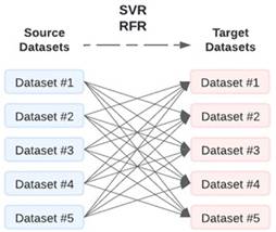
Next, to assess the transferability of SVR and RFR models in predicting LNC, new models were developed following the architecture depicted in Figure 1.

In Figure 1's architecture, each dataset employed 100% of its samples to train both an SVR and an RFR model. Thereafter, the predictive performance of each model was evaluated by estimating LNC values in the other datasets (those not used in the model development process).

Figure 1
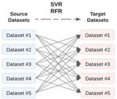
Architecture of the SVR and RFR models for evaluating the potential transferability of the predictive power of LNC between different sets of plant species.

In other words, let D = {d ₁ , d ₂ , …, d _i } be the set of datasets used in this work, and M = {m ₁ , m ₂ , …, m _i } the set of LNC prediction models developed, where I = {1,2,3,4,5}. Each model m _i was trained with data from d _i . The evaluation of m _i was based on its ability to predict LNC using reflectance samples for each element in the subset D - {d _i }.

This approach enabled investigation of the potential transferability of the predictive power of these models across different groups of plants, assessing their ability for generalization and knowledge adaptation.

In this context, the Transfer Component Analysis (TCA) algorithm was also implemented to enable the transfer of predictive capacity between the sets of reflectance values, which although different, are related to the determination of LNC.

TCA is a transfer learning algorithm proposed by Pan et al. (2008), which seeks via dimensionality reduction, to find a shared representation between different but related datasets. In this space, the distance between the data distributions of the source set and the target set was minimal, making it possible to apply common regression or classification algorithms, such as SVR and RFR. The distance between the distributions of the sets can be obtained by the maximum mean discrepancy (MMD) in a KerneL Hilbert space (RKHS). Based on this, let X _s = [x _s1 , x _s2 , …, x _sn ], and X _t = [x _t1 , x _t2 , …, x _tn ] be the sets of reflectance values of the source domain and the target domain respectively, the TCA seeks to find the projection matrix w from the following eigenvalue decomposition problem (4):

KHKw = λ(KLK+μI)w(4)

where

K= (K _s,s K _s,t K _t,s K _t,t ), K _s,s K _s,t K _t,s K _t,t are the kernel matrices, H = I - 11^T /(n _s + n _t )

and

$L_{i,j}=\{\frac{1}{n_s^2}if{x}_i,x_j\in X_s\frac{1}{n_t^2}if{x}_i,x_j\in X_t\frac{-1}{n_s{n}_t}othercases$

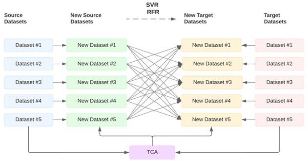
Thus, in the final analysis, transferability was evaluated for models generated by combining the TCA algorithm with SVR and TCA algorithm with RFR, as depicted in Figure 2.

In the architecture of Figure 2, each pair of datasets underwent TCA. This process resulted in the creation of newly adapted datasets with similar distributions, thereby facilitating the application of conventional machine learning algorithms. Subsequently, prediction models, RFR and SVR, were trained using one of the adapted datasets as the training set, referred to as the source dataset. Thereafter, the predictive capability of these models was evaluated using the other adapted dataset as the test set, referred to as the target dataset. This systematic procedure enabled us to observe the extent to which the adaptation provided by TCA influences the predictive capacity of the models.

Figure 2
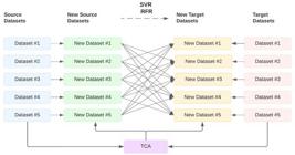
Architecture of the SVR and RFR models for evaluating the potential transferability of the predictive power of LNC between different sets of plant species, after domain adaptation by TCA.

The prediction models were evaluated using the Root Mean Square Error (RMSE) metric, which revealed the standard deviation of the residuals, i.e. a measure of the average deviation between the observed and the predicted. The square root (5) was applied so that the unit would remain on the same scale as the original data.

$RMSE\left(y,\widehat{y}\right)=\sqrt{\frac{1}{n}{\sum }_{i=1}^n{(y_i-\widehat{y_i})}^2}$(5)

where y and ŷ represent the actual and predicted LNC values, respectively, and n is the number of samples.

For the Python language, the ML library scikit-learn was used to implement the models, and the hyperparameters of the models were determined using the Grid Search Cross Validation algorithm, considering recurring values in the literature and 3 different kernel functions for the SVR (polynomial, radial basis function and sigmoid). When running the TCA, the 'primal' kernel was used with a projection to 5 dimensions, to operate non-complex numerical values.

Results and discussion

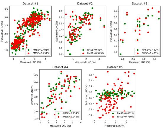
For the five SVR and RFR models developed from 75% of the data in each set, the results obtained are shown in Figure 3.

For the SVR models (in green in Figure 3), RMSE values of 0.40, 0.43, 0.48, 0.95, and 0.86% were obtained for datasets #1, #2, #3, #4, and #5, respectively. The RFR models (in red in Figure 3) obtained results very close to the SVR, with Root Mean Square Error (RMSE) values: 0.45, 0.54, 0.47, 0.94, and 0.76% for datasets #1, #2, #3, #4, and #5, respectively.

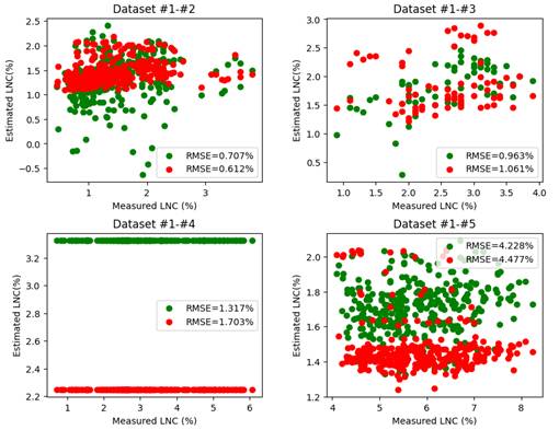
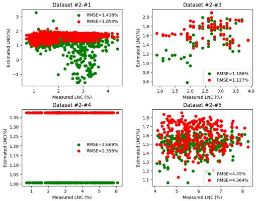
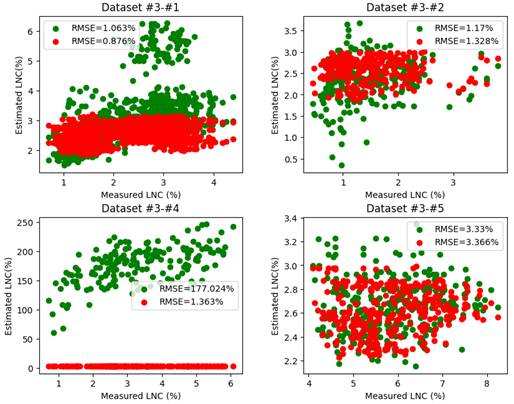
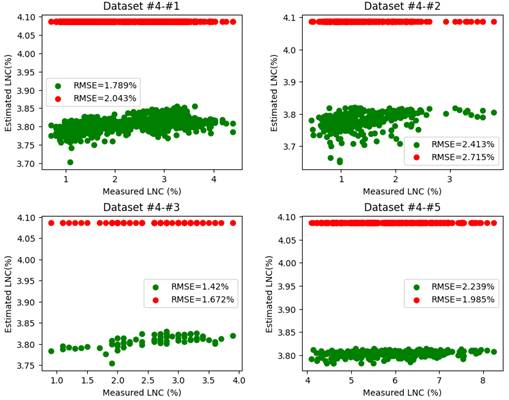
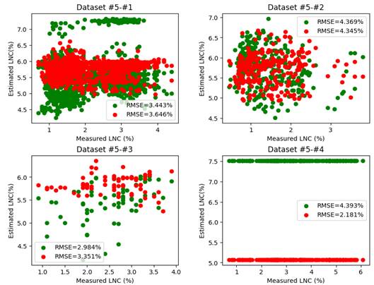
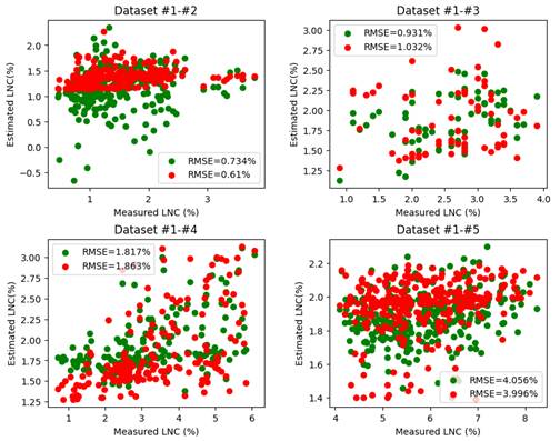
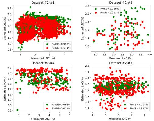
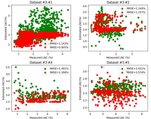
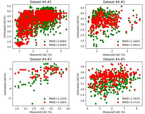
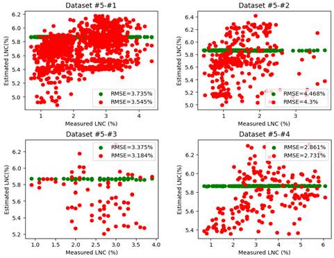
The results of the transferability analysis of the SVR and RFR models, whose proposed architecture is shown in Figure 1, are shown in Figures 4, 5, 6, 7, and 8.

None of the models generated were transferable to dataset 4, estimating a constant LNC value independent of the reflectance values.

Figure 3
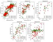
Comparative results of the SVR (in green) and RFR (in red) models in predicting leaf nitrogen concentration (LNC). For example, "Dataset #1" indicates that the SVR model is slightly more capable than the RFR model in predicting LNC for dataset #1, as it has a lower root mean square error.

Figure 4
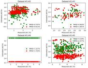
Comparative result of the transferability analysis of the SVR (in green) and RFR (in red) models developed from dataset #1. For example, "Dataset #1-#2" indicates that the RFR model trained on data from dataset #1 is slightly more capable than the SVR model at predicting LNC from dataset #2, as it obtained a lower RMSE.

Figure 5
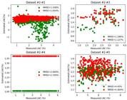
Comparative result of the transferability analysis of the SVR and RFR models developed from dataset #2.

Figure 6
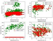
Comparative result of the transferability analysis of the SVR and RFR models developed from dataset #3.

For the SVR models, the valid RMSE values ranged from 0.70 to 4.45%, with an average RMSE value of approximately 2.32%. The highest RMSE values, above 4%, were obtained when transferring the model developed with set #1 to set #5 (RMSE = 4.22%), the model developed with set #5 to set #2 (RMSE = 4.36%), and the model developed with set #2 to set #5 (RMSE = 4.45%).

Figure 7
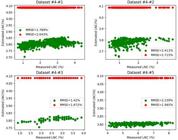
Comparative result of the transferability analysis of the SVR and RFR models developed from dataset #4.

Figure 8
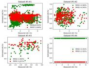
Comparative result of the transferability analysis of the SVR and RFR models developed from dataset #5.

For the RFR models, the valid RMSE values ranged from 0.61 to 4.47%, with an average RMSE value of 2.46%. The highest RMSE values, above 4%, were obtained in the same situations as the SVR models, i.e. in the transferable models from set #1 to set #5 (RMSE = 4.47%), from set #5 to set #2 (RMSE = 4.34%), and finally from set #2 to set #5 (RMSE = 4.36%).

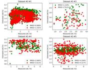
The results of the transferability analysis of the models generated from the combination of Transfer Component Analysis (TCA) with SVR and TCA with RFR algorithms, as proposed in the architecture presented in Figure 2, are shown in Figures 9, 10, 11, 12, and 13.

Figure 9
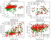
Comparative result of the transferability analysis of the SVR and RFR models developed from dataset #1 after domain adaptation provided by TCA.

Figure 10
Comparative result of the transferability analysis of the SVR and RFR models developed from dataset #2 after domain adaptation provided by TCA.

Figure 11
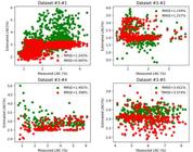
Comparative result of the transferability analysis of the SVR and RFR models developed from dataset #3 after domain adaptation provided by TCA.

Figure 12
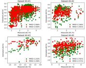
Comparative result of the transferability analysis of the SVR and RFR models developed from dataset #4 after domain adaptation provided by TCA.

After implementing the TCA, the models were transferable to all dataset combinations. For the SVR models, the valid RMSE values obtained ranged from 0.73 to 4.29%, with an average RMSE value of approximately 1.98%. For the RFR models, the RMSE values ranged from 0.61 to 4.31%, with an average RMSE value of 2.24%.

Figure 13
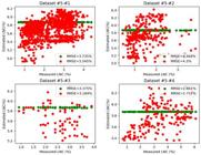
Comparative result of the transferability analysis of the SVR and RFR models developed from dataset #5 after domain adaptation provided by TCA.

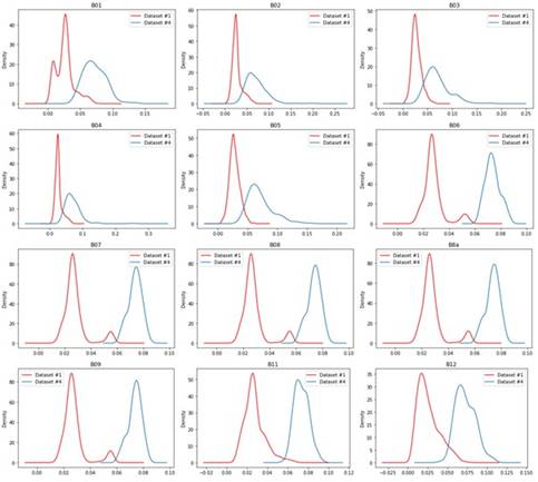
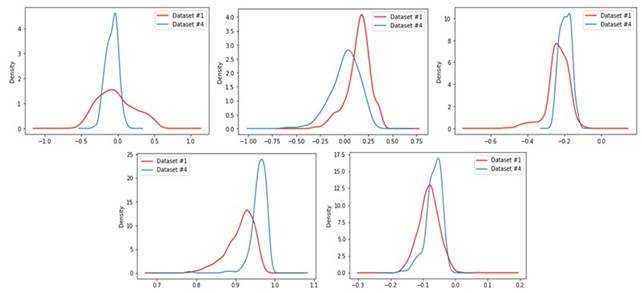
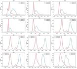
Figure 14 shows a comparison of the density graphs from datasets #1 and #4 before the TCA projection, and Figure 15 shows the new density distribution from the same sets after the TCA. The comparison proposed in the graphs provides an overview of the impact of the TCA on the adaptation of the domains of the sets.

Figure 14
Comparative density distribution of datasets #1 and #4 in the Sentinel-2 bands.

Figure 15
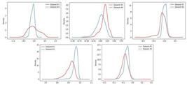
Density distribution of datasets #1 and #4 mapped into a shared representation space found by TCA.

The results obtained with the first models developed, five SVR and RFR models (Figure 3), confirmed that both SVR and RFR are good LNC estimators. This result can be easily understood since the data used for model development and validation are similar and within the same dataset. The models that did not perform satisfactorily, with the highest RMSE for both the SVR and the RFR, were those developed from dataset #4, followed by those developed from dataset #5. These datasets had the highest standard deviation related to the LNC, as presented in Table 2.

On the contrary, the results presented in Figures 4, 5, 6, 7, and 8 show that the transferability of the SVR and RFR models depends in part on the distribution of LNC and the spectral characteristics associated with different sets of plants. Dataset 5, composed of data from only one plant species, was involved in the development and validation of poor estimators, leading to overestimates and underestimates in LNC predictions. Furthermore, none of the models generated were transferable to dataset 4. This result can be attributed to the high dispersion of the data in this set, as seen in Table 2.

However, after the domain adaptation provided by TCA, transferable models were developed for all combinations of datasets. The results obtained with the SVR and RFR models after the TCA, and the density graphs of the sets shown in Figures 14 and 15, showed that the TCA effectively improved the performance of the SVR and RFR models, being able to find a shared representation between different sets of reflectance values.

In future research, it would be beneficial to investigate the reasons behind the varying performance of the SVR and RFR models across different datasets. Utilizing explainable artificial intelligence (XAI) techniques could provide deeper insights into the factors influencing model performance, thereby enhancing our understanding of model behavior and improving the applicability of these models in practical settings.

Conclusion

The spectral resampling process enabled the creation of effective LNC prediction models. This is because the combination of TCA with SVR and TCA with RFR, efficiently extracted the spectral characteristics common to the resampled leaf reflectance sets and reliably estimated the plant's LNC. It is possible to generate transferable models capable of assisting in the monitoring of plant LNC, with less investment in sampling and chemical analysis, and consequently, optimizing the decision-making process for nitrogen fertilization management in agriculture.

Data availability

The data resulting from this study are not available in public repositories, as they comprise a large volume of information, including the datasets resampled to the satellite bands, the data processed after the application of the TCA algorithm, and the prediction outputs of each model. The analyses presented from Figure 3 onward clearly and sufficiently describe the obtained results. Therefore, this item is considered not applicable.

References

• Berger, K., Verrelst, J., Féret, J., Wang, Z., Wocher, M., Strathmann, M., Danner, M., Mauser, W. & Hank, T.. (2020a). Crop nitrogen monitoring: Recent progress and principal developments in the context of imaging spectroscopy missions. Remote Sensing of Environment, 242, 111758. https://doi.org/10.1016/j.rse.2020.111758
  » https://doi.org/https://doi.org/10.1016/j.rse.2020.111758
• Berger, K., Verrelst, J., Féret, J., Hank, T., Wocher, M., Mauser, W. & Camps-Valls, G.. (2020b). Retrieval of aboveground crop nitrogen content with a hybrid machine learning method. International Journal of Applied Earth Observation and Geoinformation, 92(2020), 1-15. https://doi.org/10.1016/j.jag.2020.102174
  » https://doi.org/https://doi.org/10.1016/j.jag.2020.102174
• Cilia, C., Rossini, M., Meroni, M., Busetto, L., Amaducci, S., Boschetti, M., Picchi, V. & Colombo, R.. (2014). Nitrogen status assessment for variable rate fertilization in maize through hyperspectral imagery. Remote Sensing, 6(7), 6549-6565. https://doi.org/10.3390/rs6076549
  » https://doi.org/https://doi.org/10.3390/rs6076549
• Clevers, J. G. P. W. & Kooistra, L.. (2011). Using hyperspectral remote sensing data for retrieving canopy chlorophyll and nitrogen content. IEEE Journal of Selected Topics in Applied Earth Observations and Remote Sensing, 5(2), 574-583. https://doi.org/10.1109/JSTARS.2011.2176468
  » https://doi.org/https://doi.org/10.1109/JSTARS.2011.2176468
• Drucker, H., Burges, C. J. C., Kaufman, L., Smola, A. & Vapnik, V.. (1996). Support vector regression machines. Advances in Neural Information Processing Systems, 9, 155-161. https://papers.nips.cc/paper_files/paper/1996/file/d38901788c533e8286cb6400b40b386d-Paper.pdf
  » https://papers.nips.cc/paper_files/paper/1996/file/d38901788c533e8286cb6400b40b386d-Paper.pdf
• European Space Agency. (2019). Sentinel-2 spectral response functions (S2-SRF) (COPE-GSEG-EOPG-TN-15-0007; Version 3.0). https://sentinels.copernicus.eu/web/sentinel/user-guides/sentinel-2-msi/document-library/-/asset_publisher/Wk0TKajiISaR/content/sentinel2a-spectral-responses
  » https://sentinels.copernicus.eu/web/sentinel/user-guides/sentinel-2-msi/document-library/-/asset_publisher/Wk0TKajiISaR/content/sentinel2a-spectral-responses
• Féret, J., Berger, K., Boissieu, F. & Malenovský, Z.. (2021). PROSPECT-PRO for estimating content of nitrogen-containing leaf proteins and other carbon-based constituents. Remote Sensing of Environment, 252, 112173. https://doi.org/10.1016/j.rse.2020.112173
  » https://doi.org/https://doi.org/10.1016/j.rse.2020.112173
• Izbicki, R., & Santos, T. M. (2020). Machine learning: A statistical approach (pp. 82-88) e-book. Brazil.
• Jetz, W., Cavender-Bares, J., Pavlick, R., Schimel, D., Davis, F. W., Asner, G. P., Guralnick, R., Kattge, J., Latimer, A. M., Moorcroft, P., Schaepman, M. E., Schildhauer, M. P., Schneider, F. D., Schrodt, F., Stahl, U. & Ustin, S. L.. (2016). Monitoring plant functional diversity from space. Nature Plants, 2(3), 1-5. https://doi.org/10.1038/nplants.2016.24
  » https://doi.org/https://doi.org/10.1038/nplants.2016.24
• Lehnert, L., Meyer, H. & Bendix, J. (2022). hsdar-package: Manage, analyse and simulate hyperspectral data in R. https://rdrr.io/cran/hsdar/man/hsdar-package.html
  » https://rdrr.io/cran/hsdar/man/hsdar-package.html
• Muñoz-Huerta, R. F., Guevara-Gonzalez, R. G., Contreras-Medina, L. M., Torres-Pacheco, I., Prado-Olivarez, J. & Ocampo-Velazquez, R. V.. (2013). A review of methods for sensing the nitrogen status in plants: Advantages, disadvantages and recent advances. Sensors, 13(8), 10823-10843. https://doi.org/10.3390/s130810823
  » https://doi.org/https://doi.org/10.3390/s130810823
• Pan, S. J., Kwok, J. T. & Yang, Q.. (2008). Transfer learning via dimensionality reduction. In AAAI'08: Proceedings of the 23rd National Conference on Artificial Intelligence, 2, 677-682. https://doi.org/10.5555/1620163.1620177
  » https://doi.org/https://doi.org/10.5555/1620163.1620177
• Prey, L. & Schmidhalter, U.. (2019). Simulation of satellite reflectance data using high-frequency ground based hyperspectral canopy measurements for in-season estimation of grain yield and grain nitrogen status in winter wheat. ISPRS Journal of Photogrammetry and Remote Sensing, 149, 176-187. https://doi.org/10.1016/j.isprsjprs.2019.01.023
  » https://doi.org/https://doi.org/10.1016/j.isprsjprs.2019.01.023
• Schlemmer, M., Gitelson, A., Schepers, J., Ferguson, R., Peng, Y., Shanahan, J. & Rundquist, D.. (2013). Remote estimation of nitrogen and chlorophyll contents in maize at leaf and canopy levels. International Journal of Applied Earth Observation and Geoinformation, 25, 47-54. https://doi.org/10.1016/j.jag.2013.04.003
  » https://doi.org/https://doi.org/10.1016/j.jag.2013.04.003
• Wan, L., Zhou, W., He, Y., Wanger, T. C. & Cen, H.. (2022). Combining transfer learning and hyperspectral reflectance analysis to assess leaf nitrogen concentration across different plant species datasets. Remote Sensing of Environment, 269, 112826. https://doi.org/10.1016/j.rse.2021.112826
  » https://doi.org/https://doi.org/10.1016/j.rse.2021.112826
• Wang, S., Zhu, J., Chung, F. L., Lin, Q. & Hu, D. (2005). Theoretically optimal parameter choices for support vector regression machines with noisy input. Soft Computing, 9(10), 732-741. https://doi.org/10.1007/s00500-004-406-3
  » https://doi.org/https://doi.org/10.1007/s00500-004-406-3

Edited by

• Associate Editor in charge:
  Alessandro Lucca Braccini
  https://orcid.org/0000-0002-6915-4804
  Carlos Alberto Scapim
  https://orcid.org/0000-0002-7047-9606

Publication Dates

• Publication in this collection
  16 Mar 2026
• Date of issue
  2026

History

• Received
  31 July 2024
• Accepted
  16 Dec 2024