A mixed-effects model approach to height-diameter relationships

ABSTRACT.

Height-diameter models are widely used to estimate tree height from diameter at breast height (DBH) and play a crucial role in forest inventories by reducing fieldwork effort. However, statistical challenges such as nonlinearity, heteroscedasticity, nonnormality, and outliers can compromise model accuracy. To address these issues, this study proposes a generalization of Scolforo’s height‒diameter model (Scolforo, 1998), which incorporates random effects to improve flexibility and fit. With observational data from Eucalyptus urograndis plantations, we present a step-by-step framework for model fitting, inference, and validation. Our approach considers hierarchical structures and variability across stands to improve predictive performance. To rigorously assess model adequacy, we conducted a simulation study under various scenarios, evaluating goodness-of-fit with deviance, randomized quantile residuals, and least-confounded residuals. These diagnostics identify misspecification and enable robust parameter estimation. Additionally, we provide a detailed tutorial (Appendix B) for implementing the model in R that encompasses (i) inference for fixed and random effects, (ii) local influence analysis to detect sensitive observations, and (iii) residual-based diagnostics adapted to mixed models. Our results reveal the adaptability of the model to complex data structures while maintaining interpretability. The proposed framework provides forest researchers a reliable tool for height prediction that combines theoretical rigor and practical applicability. The accompanying R tutorial increases reproducibility and facilitates the integration of the framework into forest inventory workflows.

Keywords:
Eucalyptus; mixed effects models; height-diameter relationship; sustainable forest practices

Introduction

The cultivation of trees for industrial purposes has significantly increased in Brazil recently compared with that in many other countries (Indústria Brasileira de Árvores [IBA], 2019). Compared with that in 2020, the total area of planted trees in 2021 increased from 9.75 to 9.93 million hectares, an increase of 1.9%. Approximately 75.8% of the area is covered with Eucalyptus trees, whereas 19.4% of the area is covered with pine, totaling approximately 7.53 and 1.93 million hectares, respectively. In addition, the sector has 475k hectares of rubber tree, black wattle, teak, and parica. The planted tree sector provides economic, social, and environmental benefits by creating new local jobs and mitigating climate change (Indústria Brasileira de Árvores [IBA], 2022).

Forest inventories provide essential information for quantifying volume and biomass stocks and other variables (Scolforo, 1998). Forest plantations are affected by multiple factors because they are conducted by forestry companies in diverse locations, forest stands with various planting ages, management systems, genetic materials, and even administrative areas. These factors can be classified into hierarchical, nested structures, such as forest regions, stands, and trees. Additionally, longitudinal data are generated from the repeated measurements obtained over time on the same tree for continuous inventory. Forest inventories typically involve establishing sample plots, measuring the diameter at breast height (D) of each tree within these plots, and recording the heights (H) of the selected trees. These variables provide the information needed for forest management and decisions.

As a typical practice in inventories conducted by forestry companies, only a subset of trees is measured for both D and H For the remaining trees in the plot, all D values are measured, whereas the H values of the unmeasured trees within the plots are predicted using a height-diameter equation. This procedure can be applied in temporary, preharvest, or continuous inventories. This procedure is particularly valuable for forest management and ecological studies, and it simplifies fieldwork by reducing data acquisition costs by decreasing the time spent measuring H making the process more cost-effective and accurate while providing critical information regarding forest dynamics (Lima et al., 2021).

Height-diameter equations can be very useful, flexible, and adaptable for predicting tree height on the basis of individual or stand-level attributes. Height-diameter equations can also be affected by various factors, including stand age, basal area per hectare, crown length, mean quadratic diameter, dominant height, silvicultural practices, and geographical characteristics (Scolforo, 1998; Meng et al., 2008; Hofiço et al., 2020). There are various classes of models used for height‒diameter relationships, as reported by da Silva et al. (2024). A more complex height-diameter model is needed to incorporate the effects of the three hierarchical levels (forest region, stand, and tree) in addition to repeated measurements, such as the model proposed by Scolforo (1998). Additionally, nonnormality, nonlinear behavior, error dependence, and potential heterogeneity of variance are other aspects of tree height modeling to consider because of the biological behavior of the associated variables (H as a function of D).

The challenges in properly modeling the mean and the variance reveal the importance of selecting adequate modeling techniques to address the complex relationships inherent in forest inventory data associated with the levels of the hierarchical structure of the data-generating processes for D and H. Mixed effects models are highly flexible because they can include fixed-effect parameters to assess the relationship between a continuous dependent variable and one or more predictor variables and random effects specific to groups or units within a population to account for the correlation between repeated measurements within the same individual or between individuals within the same group. Mixed effects models consider different structures of variances and covariances in errors, providing more accurate information about the average behavior of the analyzed units (Verbeke & Molenberghs, 2000; West et al., 2022).

Mixed effects models have been increasingly applied over time, and notable examples used to analyze forestry data include those of Hofiço et al. (2020), Chenge (2021), Raptis et al. (2021), and da Silva et al. (2026). However, few studies have employed this approach to analyze data for the genus Eucalyptus, which is the target of the present research. Additionally, model checking and diagnostic analyses for the proposed models are lacking.

After the statistical technique for modeling is chosen, a critical step is to determine which effects should be included to obtain a parsimonious model that explains the data-generating process with the fewest possible number of parameters. The selection of a mixed model involves testing hypotheses about the fixed and random effects via likelihood ratio tests and information criteria such as AIC and BIC, combined with diagnostics and residual analysis. Typically, the random component is selected first, followed by the selection of the fixed component after the random component has been chosen (Verbeke & Molenberghs, 2000). After the model is chosen, fixed effects and variance components can be estimated, and random effects can be predicted.

Assessing the adequacy of the selected model for the dataset to ensure appropriate inferences requires caution. The analysis of residuals and diagnostics can be performed by using measures of local influence to detect outliers, deviance residuals, randomized quantile residuals, and least confounded residuals for checking the goodness of fit and Mahalanobis distance for checking the normality of the random effects. An important aspect is the use of computer programs with appropriate packages to fit a mixed model to a dataset with a hierarchical structure. This is still not a simple task in R software (R Core Team, 2021), and various aspects and details within appropriate packages should be elucidated to ensure that the procedure is performed correctly.

The objective of this paper is to use a mixed model with a fixed component based on Scolforo's generic model (Scolforo, 1998) to estimate H for a dataset with a hierarchical nested structure. The focus is on identifying, explaining, and addressing specific issues related to the high variability typically observed in grouped height-diameter data. This paper also presents methods to assess the quality of model fit and uses randomized quantile residuals and least confounded residuals for diagnostic analysis. Additionally, a tutorial in which R software was used to perform the analysis was developed (Appendix B).

In this study, we use specific terms to distinguish between key spatial and administrative scales. Forests refer to the forest ecosystem itself. The forest region is an administrative or ecological unit, which is a critical variable in our analysis. A forest site pertains to localized conditions that affect tree growth (e.g., soil and microclimate), whereas a farm is an operational unit that may encompass multiple stands across a municipality. These distinctions increase precision when hierarchical data levels (e.g., regions, sites, and management units) are discussed.

The paper is organized as follows: In the Materials and Methods section, a motivating case study, stemming from an observational study of trees of the species Eucalyptus urograndis, is presented, and a generalization of Scolforo's model (Scolforo, 1998), incorporating different types of random effects, is presented to analyze the data. A simulation study to evaluate the performance of the residuals for the model, considering different scenarios involving the combination of the number of trees, stands, and forest regions, is described. The Results section focuses on the application and findings of these models via the motivation dataset and presents the simulation results. The Final Considerations section provides a broader perspective on the use of mixed models in forestry sciences, highlighting their flexibility and the importance of carrying out residual analysis correctly. Additionally, the basic components of our modeling framework, linear mixed-effects models, estimation process, hypothesis testing, and residual analysis, and a tutorial with the computational routines in R software for the analyses are presented in the Supplementary Material (Appendix B).

Material and methods

Motivational data

The motivating dataset is an observational study with multistage sampling at three nested levels: forest region, stand, and tree. This dataset was supplied by Klabin S.A., and it is part of a continuous inventory of commercial plantations of the hybrid Eucalyptus urograndis. The first level, the forest region, represents a farm that may include one or more stands. A farm can span multiple locations within a municipality, depending on its total area. The second level, the stand, corresponds to the most homogeneous unit of forest cultivation, comprising trees of the same species, age, forest management, and genetic origin. The unit for forest harvesting consists of several stands. Stands are the smallest management units within a forest region, with an average area of 8 hectares, but they can reach 40 hectares. The third level, the tree, consists of individual trees cultivated within each stand. Note that the forest region level represents the effects of the forest region, the stand level represents factors related to forest management, and the tree level represents competition and other interactions among trees.

To collect data, various numbers of rectangular and permanent plots were randomly established in different stands within the forest regions. The sample units were randomly distributed through the stratified sampling process. The plot consisted of approximately 60 trees, arranged in six rows by ten plants with variable plot areas, occupying an area of 400 to 900 m². Annual data collection was conducted from the second year onward. In each plot, starting from the first row, a systematic measurement of total height was carried out for the first ten trees, which may or may not correspond solely to the first-row trees because of the presence of gaps, broken, or dead trees.

The dataset included 665 observations spread across 45 stands in 30 forest regions. The number of stands per forest region has minimum, maximum, mean, and variance equal to 1, 4, 1.57, and 0.80, respectively; 19 out of 30 regions (86.66%) have fewer than 3 stands each (Appendix A, Figure A1). The number of trees per stand has a minimum, maximum, mean, and variance equal to 12, 30, 14.77, and 12.08, respectively; 35 out of 45 stands (77.77%) have fewer than 16 trees each (Appendix A, Figure A2).

Additionally, the heights of the dominant trees were measured. Dominant trees are the 100 thickest trees per hectare, which indicates that one dominant tree is measured per 100 m² of plot area (Assmann, 1970). The direction of the expected plateau of the hypsometric curve is suggested for the dominant trees as the diameter at breast height increases da Silva et al. (2024).

In the field, the circumference at breast height (C) of all the trees was also measured. Qualitative codes were assigned to each stem to describe characteristics such as bifurcations, breakages, and curvatures. The length of each side of the plot was measured. Other dendrometric variables were calculated from the collected data, such as total height (H), diameter at breast height (D), basal area (m²), plot area (m²), number of trees per unit area (n/ha), dominant height (Hd), mean quadratic diameter of the plot (Dg), and age (I), and a summary of the statistics are presented in Table 1.

Table 1
Statistics of the analyzed variables for the hybrid Eucalyptus urograndis.

Variables	Min.	Median	Mean	Max.	SD
H (m)	5.40	25.00	23.79	39.60	8.20
Hd (m)	11.10	29.00	25.86	38.30	8.25
C (mm)	154.00	498.00	511.80	873.00	158.33
D (cm)	4.90	15.85	16.29	27.78	5.04
Dg (cm)	8.40	16.00	15.32	22.30	3.70
I (years)	1.40	4.70	4.69	8.70	2.07
Dg/D (cm)	0.65	0.92	0.98	2.95	0.24
1/D (cm)	0.03	0.06	0.06	0.20	0.02
1/(D x I)	0.004	0.01	0.02	0.09	0.01

• Note: H = total height; Hd = dominant height; C = circumference at breast height at 1.30 m above ground level; D = diameter at breast height at 1.30 m above ground level; Dg = mean square diameter of the plot; I = tree age; Min. = minimum; Max. = maximum; and SD = standard deviation.

A summary of the frequencies, considering D classes and H classes of hybrid Eucalyptus urograndis trees, is presented in Table 2.

Table 2
Frequency by diameter class and height of hybrid Eucalyptus urograndis trees.

	H (m)
D (cm)	[5.00, 10.00)	[10.00, 15.00)	[15.00, 20.00)	[20.00, 25.00)	[25.00, 30.00)	[30.00, 35.00)	[35.00, 40.00]	Total
[1.00, 5.00)	1	0	0	0	0	0	0	1
[5.00, 10.00)	9	52	9	0	0	0	0	70
[10.00, 15.00)	0	52	120	46	10	2	1	231
[15.00, 20.00)	0	6	5	32	80	54	3	180
[20.00, 25.00)	0	0	0	0	33	101	21	155
[25.00, 30.00)	0	0	0	0	0	11	17	28
[30.00, 35.00)	0	0	0	0	0	0	0	0
[35.00, 40.00]	0	0	0	0	0	0	0	0
Total	10	110	134	78	123	168	42	665

• D: diameter (cm) at breast height outside the bark (1.30 m); H: total tree height (m).

As shown in Figure 1, the scatterplot of log(H) versus log(Hd), clearly shows a linear trend. As the dominant height of the trees increases, the overall height also increases proportionally (Figure 1a). Similarly, the scatterplot of log(H) versus $\mathrm{l}\mathrm{o}\mathrm{g}\left(\frac{\mathrm{D}\mathrm{g}}{\mathrm{D}}\right)$ indicates an approximately linear decreasing trend, which means that as Dg/D increases, the height of the trees tends to decrease (Figure 1b). With respect to the relationships between log(H) and $\frac{1}{\mathrm{D}\mathrm{*}\mathrm{I}}$ (Figure 1c), between log(H) and 1/D (Figure 1d) and between log(H) and log(I) (Figure 1e), a nonlinear decreasing relationship is observed. As $\frac{1}{\mathrm{D}\mathrm{*}\mathrm{I}}$ and 1/D increase, log(H) tends to decrease. Moreover, the relationship between log(D) and log(I) exhibits an approximately linear trend; that is, the D of the trees tends to increase proportionally with the age of the trees (Figure 1f).

Figure 1
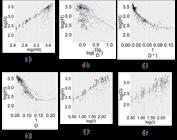
Comparative scatterplots that show the relationships between log(H) as a function of (a) Log(Hd), (b), $\mathrm{l}\mathrm{o}\mathrm{g}\left(\frac{\mathrm{D}\mathrm{g}}{\mathrm{D}}\right)$ (c), $\frac{1}{\mathrm{D}\mathrm{*}\mathrm{I}}$ (d), $\frac{1}{\mathrm{D}}$ and (e) log(I) and Log(D) as a function of (f) Log(I).

The relationships between total height (H) and diameter (D) for trees grouped by age class are shown in Figure 2. As age increases, both height and diameter tend to increase, indicating a positive correlation. Variability in the data also increases with age, revealing differences in growth conditions.

Figure 2
Total height (H) (m) as a function of diameter (D) (cm) grouped by age class.

In the following subsections, we describe the height-diameter model with fixed effects, where total height (H) is modeled as a function of several predictor variables, including diameter at breast height (D), dominant height (Hd), mean quadratic diameter (Dg), and other stand- and tree-level characteristics. A foundational overview of mixed models, including their definitions, parameter estimation, model selection, and model checking, which are important for the development and evaluation of height-diameter models that incorporate random effects, is presented in the Supplementary Materials (Appendix B).

Height-diameter model - fixed and mixed scolforo model

In this study, an initial fixed-effects model was designed as suggested by Scolforo (1998), considering log(H) as a function of the variables log(Hd), $\text{log}\left(\frac{\mathrm{D}\mathrm{g}}{\text{D}}\right)$, $\frac{\text{1}}{\text{D*I}}$ and $\frac{\text{1}}{\text{D}}$. These variables represent the effect of site conditions, age, and stand characteristics on tree height, considering that tree height is affected primarily by site quality, whereas diameter is affected by both site and competition effects. The model considers the variability in tree growth patterns and structural differences among stands and regions and represents population-wide trends, such as the relationship between dominant height and diameter.

The observational data are assumed to be derived from R forest regions with n_r stands, each containing m_rs trees, where the total height (H) and diameter at breast height (D) are measured for the i-th tree within the s-th stand of the r-th forest region. The first model (M1) with Equation (1) for Y_rsi = log(H_rsi), i = 1, …, m_rs, r = 1, …, R, and s = 1, …, n_r, assuming a normal distribution for the error, that is, ϵ_rsi ~ N(0, σ²), is presented in Table 3.

Table 3
Models considered to analyze the Eucalyptus dataset.

Names	Equations	Number
M1	${\text{Y}}_{\text{rsi}}=\mathrm{}{\text{β}}_{\text{0}}\text{+}{\text{β}}_{\text{1}}\text{log}\left(\text{H}{\text{d}}_{\text{rsi}}\right)\text{+}{\text{β}}_{\text{2}}\text{log}\left(\frac{\text{D}{\text{g}}_{\text{rsi}}}{{\text{D}}_{\text{rsi}}}\right)\text{+}{\text{β}}_{\text{3}}\frac{\text{1}}{{\text{D}}_{\text{rsi}}\text{*}{\text{I}}_{\text{rsi}}}\text{+}{\text{β}}_{\text{4}}\frac{\text{1}}{{\text{D}}_{\text{rsi}}}\text{+}{\text{ϵ}}_{\text{rsi}}$	(1)
M2	${\mathrm{Y}}_{\mathrm{r}\mathrm{s}\mathrm{i}}\text{= (}{\text{β}}_{\text{0}}\text{+}{\text{u}}_{\text{1r}}\text{+}{\text{u}}_{\text{2(r)s}}\text{) +}{\text{β}}_{\text{1}}\text{log}\left(\text{H}{\text{d}}_{\text{rsi}}\right)\text{+}{\text{β}}_{\text{2}}\text{log}\left(\frac{\text{D}{\text{g}}_{\text{rsi}}}{{\text{D}}_{\text{rsi}}}\right)\text{+}{\text{β}}_{\text{3}}\frac{\text{1}}{{\text{D}}_{\text{rsi}}\text{*}{\text{I}}_{\text{rsi}}}\text{+}{\text{β}}_{\text{4}}\frac{\text{1}}{{\text{D}}_{\text{rsi}}}\text{+}{\text{ϵ}}_{\text{rsi}}\mathrm{}\mathrm{}$	(2)
M3	${\mathrm{Y}}_{\mathrm{r}\mathrm{s}\mathrm{i}}\text{= (}{\text{β}}_{\text{0}}\text{+}{\text{u}}_{\text{1r}}\text{) +}{\text{β}}_{\text{1}}\text{log}\left(\text{H}{\text{d}}_{\text{rsi}}\right)\text{+}{\text{β}}_{\text{2}}\text{log}\left(\frac{\text{D}{\text{g}}_{\text{rsi}}}{{\text{D}}_{\text{rsi}}}\right)\text{+}{\text{β}}_{\text{3}}\frac{\text{1}}{{\text{D}}_{\text{rsi}}\text{*}{\text{I}}_{\text{rsi}}}\text{+}{\text{β}}_{\text{4}}\frac{\text{1}}{{\text{D}}_{\text{rsi}}}\text{+}{\text{ϵ}}_{\text{rsi}}\mathrm{}\mathrm{}$	(3)
M4	${\mathrm{Y}}_{\mathrm{r}\mathrm{s}\mathrm{i}}\text{= (}{\text{β}}_{\text{0}}\text{+}{\text{u}}_{\text{2(r)s}}\text{) +}{\text{β}}_{\text{1}}\text{log}\left(\text{H}{\text{d}}_{\text{rsi}}\right)\text{+}{\text{β}}_{\text{2}}\text{log}\left(\frac{\text{D}{\text{g}}_{\text{rsi}}}{{\text{D}}_{\text{rsi}}}\right)\text{+}{\text{β}}_{\text{3}}\frac{\text{1}}{{\text{D}}_{\text{rsi}}\text{*}{\text{I}}_{\text{rsi}}}\text{+}{\text{β}}_{\text{4}}\frac{\text{1}}{{\text{D}}_{\text{rsi}}}\text{+}{\text{ϵ}}_{\text{rsi}}\mathrm{}\mathrm{}$	(4)
Yrsi = log(Hrsi), u1r ~ N(0, σ2 1), u2(r)s ~ N(0, σ2 2), ϵrsi ~ N(0, σ2), i = 1, …, mrs, r = 1, …, R, s = 1, …, nr

To consider the hierarchical structure of the data and correlations between stands within regions and between trees within stands, independent random effects u_1r ~ N(0, σ² ₁) and u_2(r)s ~ N(0, σ² ₂) for forest regions and stands, respectively, can be integrated into Equation (1). A general mixed-effect model (M2) is represented by Equation (2) in Table 3. This approach can increase prediction accuracy, making the models indispensable for forest management, inventories, and research (Verbeke & Molenberghs, 2000).

Considering the forest region as a random effect allows the correlation between stands within a region to be modeled, ${\mathrm{\rho }}_{\text{(r)s}}=\mathrm{}\frac{{\mathrm{\sigma }}_1^2}{{\mathrm{\sigma }}_1^2+{\mathrm{\sigma }}_2^2+{\mathrm{\sigma }}_{\mathrm{ϵ}}^2}$, whereas a random effect for stands within regions allows the correlation between trees within stands to be modeled, ${\mathrm{\rho }}_{\text{(rs)i}}=\mathrm{}\frac{{\mathrm{\sigma }}_1^2+{\mathrm{\sigma }}_2^2}{{\mathrm{\sigma }}_1^2+{\mathrm{\sigma }}_2^2+{\mathrm{\sigma }}_{\mathrm{ϵ}}^2}$. However, for the motivation dataset, 86.66% of the regions contain fewer than four stands each, which hinders the precise estimation of variance components. This finding occurs because the variability between regions is partially confounded by the variability among stands within the regions. In these cases, simpler models could be used, either by considering random effects only for forest regions (M3) or for stands (M4), as shown in Table 3.

Hypothesis testing, diagnostics, and residual analysis

Designing a mixed model involves determining which random and fixed effects should be included. Generally, the random component is initially selected, and then the fixed component is selected on the basis of the chosen random component. To determine which random effects should be included in the model, Wald tests and likelihood ratio tests (ML and REML) can be used for inferences about the components of variance for two nested models having the same set of fixed-effect parameters but different sets of random-effect parameters (Appendix B).

To compare the models (M1-M4), we test hypotheses about the components of variance, as shown in Table 6. We use the restricted maximum likelihood ratio (REML) test, as well as their corresponding Akaike information criterion (AIC) and conditional AIC (cAIC) values. This approach involves tests in the limit of the parametric space, with the difference of loglikelihoods at maximum having a mixture of (² distributions (Appendix B). An important step in statistical modeling is the diagnostics and analysis of residuals, which assesses the adequacy of the selected model for the dataset. Various graphical techniques can be used to informally assess the goodness of fit of a model. We highlight the half-normal plot with a simulated envelope (Atkinson, 1985).

After a linear mixed model is fit to a dataset, three types of residuals can be calculated to evaluate the extra variability present in the data on the basis of the marginal model, conditional model, and random effects (Appendix B). However, they are not suitable for diagnostics, because they are difficult to interpret when different variances are allowed in the model; these can be correlated even for uncorrelated data (Nobre & Singer, 2007). Another point to highlight is that residuals that exhibit dependence on some additional source of variation in their functions are called confounded residuals, including, for example, conditional residuals, ${\widehat{\text{r}}}_{\text{c}}$ that exhibit confounding with the vector of random effects parameters (Hilden-Minton, 1995). Least-confounded residuals, as proposed by Hilden-Minton (1995), were specifically designed to decrease confounding among sources of variation in linear mixed-effects models.

These residuals can be used to obtain a quantile‒quantile plot with a simulated envelope to verify the assumption of normality of the conditional errors (Atkinson, 1985; Hinde & Demétrio, 1998; Moral et al., 2017; Singer et al., 2017). Randomized quantile residuals were proposed by Dunn and Smyth (1996) as an alternative to other types of residuals. Another type of residual is the deviance residual (Cordeiro et al., 2024). To verify the assumption of normality of the random effects, Singer et al. (2017) suggest constructing a QQ plot based on the Mahalanobis distance proposed by Waternaux et al. (1989). Cook (1986) presented the idea of local influence to investigate how subtle changes in a model can affect the analysis. For example, these changes can be made to the covariance matrix, parameters, or response variable. A slightly different and more practical approach to local influence diagnostics in linear mixed models is considered by Beckman et al. (1987) and Lesaffre and Verbeke (1998).

Let (^ be the parameter estimate considering all the observations and (^_(i) be the estimate without the i-th observation. To evaluate the effect of deleting an observation on the parameter estimates ((^, (^_(i)), the mixed model is fitted for both the complete dataset and for the dataset after the i-th outlier observation is removed. The estimates of the fixed effects parameters and variance components from both models are extracted, and the value of $\left[\frac{\left({\widehat{\mathrm{\theta }}}_{\left(\mathrm{i}\right)}-\mathrm{}\widehat{\mathrm{\theta }}\right)}{\widehat{\mathrm{\theta }}}\times 100\mathrm{\%}\right]$ is obtained, where (^_(i) represents the estimate without the i-th observation (Nobre & Singer, 2007) with the computational routines developed by Nobre (2026).

Simulation study

Simulation studies in mixed-effects models to evaluate the properties of residuals under different scenarios for different types of data have been widely applied in the literature (Schützenmeister & Piepho, 2012; Loy, 2013; Bani-Mustafa et al., 2019). However, the literature indicates the prevalent use of deviance and randomized quantile residuals for this class of models. For this study, a simulation was conducted with the primary objective of comparing the performance of the deviance residuals, randomized quantile residuals, and least-confounded residuals.

Data generation approach

The dataset is generated using, as parameters, the estimates obtained from the fitting model (M4) to the Eucalyptus urograndis data. The following values for the variance components are assumed: for forest stands, (_s ² = 0.002; the residual variance (_ϵ ² = 0.005. For the fixed effects, the following values were used: β₀ = 0.32, β₁ = 0.91, β₂ = -0.48, β₃ = 3.38 and β₄ = -3.43. We considered different scenarios on the basis of combinations of the following factors:

for forest stands, (_s ² = 0.002; the residual variance (_ϵ ² = 0.005. For the fixed effects, the following values were used: β₀ = 0.32, β₁ = 0.91, β₂ = -0.48, β₃ = 3.38 and β₄ = -3.43.

Scenario 1 (number of factor levels fixed): number of forest regions (10, 15, and 30), number of stands per region (2, 4, and 6) and number of trees per stand (10, 20, and 30).

Scenario 2 (number of factor levels not fixed): fixed number of forest regions (10, 15, and 30), with the number of stands per region generated from a Poisson distribution with mean λ= (2 and 4) and the number of trees per stand generated from a Poisson distribution with mean λ= (10, 20 and 30) to represent the degree of forest structure heterogeneity.

For each combination, 500 replicates were generated. The tree diameter at breast height (D) and tree height (H) were simulated using a bivariate model for [log (D), log (H)] as a function of log (I). The ages of the trees were generated from a uniform distribution, U(1,9). The parameters for the covariance matrix of residuals ( of the bivariate model were obtained from a multivariate analysis of variance (MANOVA) fitted to the Eucalyptus urograndis data. The dominant height (Hd) and mean quadratic diameter (Dg) were computed for each stand on the basis of the simulated tree-level values of H and D.

A linear mixed model (M4 as presented in the Results) was used to simulate the response variable (tree total height), because this indicated excellent performance in capturing data variability and provided the best fit compared with alternative models.

Fitting the models and evaluation

For each generated dataset, (M4) was fitted. Residual diagnostics were calculated for each fitted model, focusing on three types of residuals: randomized quantile residuals, deviance residuals, and least-confounded residuals. For each type of residual, half-normal plots were generated, and the percentage of points falling outside the 5% confidence envelopes was recorded. The results were stored for each simulation and aggregated across all combinations to evaluate the model performance under varying fixed factor conditions, as follows:

Scenario 1 (number of factor levels fixed): Each residual type was labeled accordingly, and the percentages were plotted as grouped bar charts to show the performance of the residual diagnostics across all combinations. The combinations of factors are represented along the x-axis, while the percentage of residuals within the 5% threshold are shown on the y-axis.

Scenario 2 (number of factor levels not fixed): The same threshold-based approach was used, and the results were reorganized into a long-format structure in grouped bar charts. However, Scenario 2 used an additional layer of analysis to consider the variations in sample sizes generated by the Poisson-distributed numbers of stands and trees. To ensure a fair comparison across the combinations, the total number of residuals for each replicate was divided into sample size classes. These classes were defined on the basis of intervals of total data points, representing the variability in the number of observations. The classes allowed for stratified evaluation of model performance. For each sample size class within a given combination, the percentage of residuals falling within the 5% threshold was calculated separately for the residuals. The results are shown in grouped bar charts, where the x-axis represents the sample size classes and the y-axis represents the percentage of residuals within the threshold. This stratified approach allowed for a robust and unbiased evaluation of model performance, considering the inherent variability introduced by the Poisson-distributed generation of stands and trees.

Computational aspects

The system specifications used to run our methods included a Windows 10 operating system and an Intel Core i5-7200U processor with 2 cores, 4 threads, and 16 GB of RAM. The analysis of the motivating data was carried out with R software (version 4.1.2; R Core Team, 2021). The models were fitted via the lme() function from the nlme package (Pinheiro, 2011). Therefore, the function asreml of the asreml package of Butler et al. (2009) or the mmer() function from the sommer package version 4.3.1 can be used (Covarrubias-Pazaran, 2016). To obtain the conditional AIC values, we used the cAIC4 package of Säfken et al. (2021). The Wald F test for fixed effects was conducted via the wald() function from the ASReml package (Butler et al., 2009). Computational routines developed by Nobre (2026) were applied to obtain the least confounded residuals. In the simulation study, half-normal plots with simulated envelopes generated via the hnp package were used (Moral et al., 2017).

Results and discussion

Models

The Eucalyptus urograndis data, as well as the corresponding R code for fitting the models, were formatted and are presented in Box 1 (Appendix D). The values for the loglikelihood at maximum (logLik), AIC and cAIC for Models M1 to M4 are summarized in Table 4 and are shown in Box D1 (Appendix D). Note that the model (M4) with random effects per stand is the best model.

Table 4
Results of fitting several models to Eucalyptus urograndis data, using the same fixed effects, with and without random effects.

	Complete data			Data without observation # 509
Models	logLik	AIC	cAIC	logLik	AIC	cAIC
M1	612.83	-1213.67	-	702.44	-1392.9	-
M2	636.68	-1275.36	-1302.94	738.10	-1485.21	-1501.59
M3	637.87	-1261.75	-1312.86	736.09	-1458.17	-1513.64
M4	644.35	-1277.58	-1341.40	756.47	-1498.95	-1578.58

Initial diagnostics and residual analysis

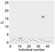
The dispersion plots of the least confounded residuals versus fitted values (Appendix C, Figure C1) and the fit of the four Models M1 to M4 to the complete dataset reveal an atypical observation. The next step is to understand the characteristics of this observation and to analyze the effect of removing it on the parameter estimates. Considering the (M4) model, when the modified Lesaffre-Verbeke index (C_i) was used, the outlier observation was in stand 35 (Q4A), as shown in Figure 3. The measurements of the individuals of stand 35 indicated that the outlier was tree #509, which had a height of 5.4 m and a D of 8.37 cm and was classified as bifurcated, and that this tree could be removed from the dataset.

Figure 3
Index plot of total local influences C_i of the individuals per stand.

To analyze the effect of observation #509, the relative changes in the parameters were calculated using the computational procedures described in Box D2 (Appendix D), and the results are presented in Table 5. When we remove tree #509, we discover that for the fixed-effect parameters, the estimates of β₁ and β₂ increase by 3.37% and 7.43%, respectively. On the other hand, the estimates of the parameters β₃ and β₄ decrease by 12.13% and 24.93%, respectively. Considering the estimates of the random effects parameters, (_s ² decreases by 4.27% when we eliminate observation #509. Therefore, tree #509 has a strong effect on the estimates of the fixed- and random-effect parameters.

The logLik, AIC and cAIC of the fitted models after observation #509 is removed are summarized in Table 3, which shows that the model (M4) still appears to be the best model.

Table 5
Estimates (± estimated standard errors) and relative changes in the parameters of the model (M4) fitted to the complete dataset and without tree #509.

Parameters	$\widehat{{\mathrm{\beta }}_0}$	$\widehat{{\mathrm{\beta }}_1}$	$\widehat{{\mathrm{\beta }}_2}$	$\widehat{{\mathrm{\beta }}_3}$	$\widehat{{\mathrm{\beta }}_4}$
Complete data	0.26±0.17	0.93±0.04	-0.47±0.06	4.45±1.15	-3.89±0.98
After tree #509 is removed	0.11±0.15(-58.65%)	0.96±0.03(3.37%)	-0.50±0.05(7.43%)	3.91±1.08(-12.13%)	-2.92±0.88(-24.93%)
Parameters	$\widehat{{\mathrm{\sigma }}_{\mathrm{s}}^2}$	$\widehat{{\mathrm{\sigma }}_{\mathrm{ϵ}}^2}$	-	-	-
Complete data	0.002420±0.000601	0.007412±0.0004	-	-	-
After tree #509 is removed	0.002528±0.000672(-4.27%)	0.005312±0.0002(39.53%)	-	-	-

Model selection for random effects

Hypothesis testing for model comparisons, as shown in Box D3 (Appendix D), is summarized in Table 6. Comparisons between the mixed-effects models (M3 and M4) and the fixed-effects model (M1) support the inclusion of random effects either by forest region or by stand (Table 6) for both the full dataset and the dataset, excluding observation #509. The remaining model comparisons did not yield significant results. The exclusion of observation #509 was justified by its undue influence on model fit, as shown in Table 5. After its removal, Model M4 (with random effects per stand) achieved the best performance, as indicated by the lowest AIC and cAIC values (Table 4) and improved residual diagnostics. Thus, M4 was selected as the optimal model and is used hereafter.

Table 6
Summary of the results for the comparison of linear mixed models.

Comparisons	Hypothesis		LR test (p value)
M1.1 vs. M3.1 M1.2 vs. M3.2	${\mathrm{H}}_{\mathrm{0,1}}:$ $\begin{array}{c}{\mathrm{D}}_0=\left[0\right]\\ {\mathrm{D}}_1=\left[{\mathrm{\sigma }}_1^2\right]\end{array}$		50.09 (<0.001) 67.28 (<0.001)
M1.1 vs. M4.1 M1.2 vs. M4.2	${\mathrm{H}}_{\mathrm{0,1}}:$ $\begin{array}{c}{\mathrm{D}}_0=\left[0\right]\\ {\mathrm{D}}_1=\left[{\mathrm{\sigma }}_2^2\right]\end{array}$		63.05 (<0.001) 108.05 (<0.001)
M2.1 vs. M3.1 M2.2 vs. M3.2	${\mathrm{H}}_{\mathrm{1,2}}:\begin{array}{c}{\mathrm{D}}_1=\left[{\mathrm{\sigma }}_1^2\right]\\ {\mathrm{D}}_2=\left[\begin{array}{cc}{\mathrm{\sigma }}_1^2& 0\\ 0& {\mathrm{\sigma }}_2^2\end{array}\right]\end{array}$		-2.38 (0.99) 4.02 (0.22)
M2.1 vs. M4.1 M2.2 vs. M4.2	${\mathrm{H}}_{\mathrm{1,2}}:\mathrm{}\begin{array}{c}{\mathrm{D}}_1=\left[{\mathrm{\sigma }}_2^2\right]\\ {\mathrm{D}}_2=\left[\begin{array}{cc}{\mathrm{\sigma }}_1^2& 0\\ 0& {\mathrm{\sigma }}_2^2\end{array}\right]\end{array}$		-15.34 (0.99) -36.74 (0.99)

• 1 and 2 indicate that the models were fit to the complete dataset and to the dataset without observation #509, respectively.

Model selection for fixed effects

After the random part of the model was selected, the Wald-F test can be used to select the fixed effects in the model (M4), with the denominator degrees of freedom estimated using the Kenward and Roger (1997) method. The results are presented in Box D4 (Appendix D) and summarized in Table 7. The results of the Wald-F tests for the fixed effects are significant at the 5% level, indicating that all the covariates in the linear predictor are needed.

Table 7
Results of Wald tests for fixed effects.

Effects	Sum Sq	Mean Sq	NumDF	DenDF	F value	p value
$\text{log}\left(\text{Hd}\right)$	3.59	3.59	1	364.15	704.80	<0.001
$\text{log}\left(\frac{\text{Dg}}{\text{D}}\right)$	0.43	0.43	1	509.52	86.05	<0.001
$\frac{\text{1}}{\text{D*I}}$	0.05	0.05	1	133.30	10.07	0.001
$\frac{\text{1}}{\text{D}}$	0.04	0.04	1	343.36	8.81	0.003

Diagnostics and residual analysis after the removal of observation #509

The graphs of the least confounded residuals of the model (M4) shown in Figure 4 that the dispersion plot of least confounded residuals versus fitted values appears homogeneous after observation #509 is removed (Figure 4a). Additionally, the histogram of the least confounded residuals shows symmetry and a mean of approximately zero (Figure 4b), indicating that the assumption of normality is unlikely to be rejected. Additionally, there are no issues related to the normality of the random effects (Figure 4c).

Figure 4
(a) Dispersion plot for the least confounded residuals vs. fitted values, (b) histogram of the least confounded residuals, and (c) quantiles of ( ² vs. the Mahalanobis quantile distance.

In this study, there is no lack of fit issue when the proposed Model (M4) is used after the removal of observation #509 to estimate the height of Eucalyptus urograndis trees. However, employ appropriate techniques for diagnostic analyses in regression models, especially in mixed effects models, as recommended by Hilden-Minton (1995) and Nobre and Singer (2007), is important. This aspect is often overlooked in the literature across various fields. However, the example presented in this study can be particularly useful for forest modeling, in height-diameter relationships and in other contexts, such as volume and biomass equations.

Results of the simulation study

Scenario 1

As shown in Figure 5, the results indicate that the least-confounded residuals consistently achieved the highest percentage of values falling within the 5% threshold across all combinations of factors, with percentages ranging from 87 to 93%. The randomized quantile residuals, with percentages typically approximately 70 to 75%, also show stable performance across combinations of forest regions, stands, and trees. In contrast, the deviation residuals presented greater variability and the lowest percentages, ranging from 66 to 74%, indicating a comparatively worse result. This finding highlights the robustness and reliability of the least-confounded residuals as a diagnostic tool for evaluating the adequacy of a fitted mixed model under fixed-factor conditions.

Figure 5
Percentages of residuals within the 5% threshold across fixed factor combinations in Scenario 1.

Scenario 2

Despite differences across the combinations of forest regions, stands, and trees, as shown in Figure 6, the results indicate that the least-confounded residuals consistently achieved the highest percentage of values within the 5% threshold across all the combinations of factors. The randomized quantile residuals also show stable performance across combinations. In contrast, the deviation residuals consistently presented more variability and consistently lower performance, indicating a relatively weaker adherence to the 5% threshold criterion. This finding emphasizes the robustness and reliability of the least-confounded residuals in evaluating mixed-model adequacy under various conditions of forest regions, stands, and trees.

Figure 6
Percentages of residuals within the 5% threshold across nonfixed factor combinations in Scenario 2.

Additionally, the results were classified according to sample sizes, from Appendix C (Figure C2), which revealed that the least-confounded residuals achieve the highest performance and that the randomized quantile residuals, in general, outperform the deviation residuals, with the exception of the second sampling classes. As the size of the sampling class increases, the ranking of the residuals shifts slightly. Overall, these findings highlight the reliability of the least-confounded residual across all the sampling classes. The randomized quantile residual exhibits strong performance in larger sampling classes. These results highlight the importance of considering the sample class size when the most appropriate residual for the analysis is selected.

Conclusion

In this study, a mixed-effects model was applied to analyze height‒diameter relationships in Eucalyptus urograndis plantations in Brazil. The model incorporated fixed effects for flexible height estimation and random effects to consider stand-level variability, improving the representation of intraindividual variation. Model selection (M4) was based on likelihood ratio tests, AIC/BIC, and Wald tests, confirming significant fixed effects. Diagnostic checks using least-confounded residuals confirmed normality and homoscedasticity, emphasizing the need for proper residual analysis in mixed models-a novel approach in forestry research. No studies have conducted these diagnostics for mixed models in forest data, which is consistent with Hilden-Minton (1995) and Singer et al. (2017), who stress addressing residual confounding and outlier influence. Fitting hierarchical models in R (via nlme and lme4) posed challenges but yielded reliable results, emphasizing the need for technical expertise. A simulation study demonstrated the superiority of least-confounded residuals over conventional methods. This work provides a framework for fitting mixed-effects models in forestry that combines robust diagnostics and practical guidance. The study highlights the importance of residual analysis, model selection, and software tools and provides valuable insights for researchers working with hierarchical forest data.

Data availability

The dataset used and analyzed in this study is not publicly available due to internal project restrictions. The supplementary material can be accessed at this link: https://drive.google.com/file/d/1GIewysbbApKgXxjslgULdQ-aqzjm_Zlu/view?usp=sharing

Acknowledgements

We acknowledge the financial support from Coordination for the Improvement of Higher Education Personnel - CAPES and National Council for Scientific and Technological Development - CNPq (No. 141409/2020-7) and CNPq Project: 312645/2021-0, Brazil for Clarice G. B. Demétrio. We acknowledge the University of São Paulo and the Universiteit Hasselt for their research support.

References

• Assmann, E. (1970). The principles of forest yield study: studies in the organic production, structure, increment and yield of forest stands. Pergamon Press.
• Atkinson, A. C. (1985). Plots, transformations, and regression an introduction to graphical methods of diagnostic regression analysis. Oxford University Press.
• Bani-Mustafa, A., Matawie, K. M., Finch, C. F., Al-Nasser, A. & Ciavolino, E.. (2019). Recursive residuals for linear mixed models. Quality & Quantity, 53, 1263-1274. https://doi.org/10.1007/s11135-018-0814-6
  » https://doi.org/https://doi.org/10.1007/s11135-018-0814-6
• Beckman, R. J., Nachtsheim, C. J. & Cook, R. D.. (1987). Diagnostics for mixed-model analysis of variance. Technometrics, 29(4), 413-426. https://doi.org/10.2307/1269452
  » https://doi.org/https://doi.org/10.2307/1269452
• Butler, D. G., Cullis, B. R., Gilmour, A. R. & Gogel, B. J. (2009). Mixed models for S language environments: ASReml-R reference manual. ASReml estimates variance components under a general linear mixed model by residual maximum likelihood. Department of Primary Industries and Fisheries.
• Cook, R. D.. (1986). Assessment of local influence. Journal of the Royal Statistical Society: Series B Statistical Methodology, 48(2), 133-155. https://doi.org/10.1111/j.2517-6161.1986.tb01398.x
  » https://doi.org/https://doi.org/10.1111/j.2517-6161.1986.tb01398.x
• Cordeiro, G. M., Demétrio, C. G. B. & Moral, R. D. A. (2024). Modelos lineares generalizados e aplicações. Blucher.
• Covarrubias-Pazaran, G.. (2016). Genome-assisted prediction of quantitative traits using the R package sommer. PLoS ONE, 11(6), 1-15. https://doi.org/10.1371/journal.pone.0156744
  » https://doi.org/https://doi.org/10.1371/journal.pone.0156744
• Chenge, I. B.. (2021). Height-diameter relationship of trees in Omo strict nature forest reserve, Nigeria. Trees, Forests and People, 3, 100051. https://doi.org/10.1016/j.tfp.2020.100051
  » https://doi.org/https://doi.org/10.1016/j.tfp.2020.100051
• Silva, B. G., Demétrio, C. G. B., Sermarini, R. A., Molenberghs, G., Verbeke, G., Behling, A., Marques, E. & Figura, M. A.. (2024). Height-diameter models: a comprehensive review with new insights on relationships to generalized linear models and differential equations. International Forestry Review, 26(4), 398-419. https://doi.org/10.1505/146554824839334687
  » https://doi.org/https://doi.org/10.1505/146554824839334687
• Silva, B. G., Demétrio, C. G. B., Sermarini, R. A., Behling, A., Molenberghs, G., Verbeke, G., Marques, E. & Figura, M. A.. (2026). Modeling Pinus tree taper data using mixed-effects models. Journal of Forestry Research, 37(1), 75. https://doi.org/10.1007/s11676-026-01985-5
  » https://doi.org/https://doi.org/10.1007/s11676-026-01985-5
• Dunn, P. K. & Smyth, G. K.. (1996). Randomized quantile residuals. Journal of Computational and Graphical Statistics, 5(3), 236-244. https://doi.org/10.1080/10618600.1996.10474708
  » https://doi.org/https://doi.org/10.1080/10618600.1996.10474708
• Hilden-Minton, J. A. (1995). Multilevel diagnostics for mixed and hierarchical linear models. University of California. https://hdl.handle.net/10568/81585
  » https://hdl.handle.net/10568/81585
• Hinde, J. & Demétrio, C. G. B.. (1998). Overdispersion: models and estimation. Computational Statistics & Data Analysis, 27(2), 151-170. https://doi.org/10.1016/S0167-9473(98)00007-3
  » https://doi.org/https://doi.org/10.1016/S0167-9473(98)00007-3
• Hofiço, N. S. A., Costa, E. A., Fleig, F. D., Finger, C. A. G. & Hess, A. F.. (2020). Height-diameter relationships for Eucalyptus grandis Hill ex. Maiden in Mozambique: using mixed-effects modeling approach. Cerne, 26(2), 183-192. https://doi.org/10.1590/01047760202026022677
  » https://doi.org/https://doi.org/10.1590/01047760202026022677
• Indústria Brasileira de Árvores. (2019). Relatório 2019 Indústria Brasileira de Árvores. IBA. https://iba.org/datafiles/publicacoes/relatorios/iba-relatorioanual2019
  » https://iba.org/datafiles/publicacoes/relatorios/iba-relatorioanual2019
• Indústria Brasileira de Árvores. (2022). Relatório 2022 Indústria Brasileira de Árvores. IBA. https://www.iba.org/datafiles/publicacoes/relatorios/relatorio-anual-iba2022
  » https://www.iba.org/datafiles/publicacoes/relatorios/relatorio-anual-iba2022
• Kenward, M. G. & Roger, J. H.. (1997). Small sample inference for fixed effects from restricted maximum likelihood. Biometrics, 53(3), 983-997. https://doi.org/10.2307/2533558
  » https://doi.org/https://doi.org/10.2307/2533558
• Lesaffre, E. & Verbeke, G.. (1998). Local influence in linear mixed models. Biometrics, 54, 570-582. https://doi.org/10.2307/3109764
  » https://doi.org/https://doi.org/10.2307/3109764
• Lima, R. B., Görgens, E. B., Elias, F., Abreu, J. C., Baia, A. L., Oliveira, C. P., Silva, D. A. S., Batista, A. P. B., Lima, R. C., Sotta, E. D., Ferreira, R. L. C., Silva, J. A. A. & Carneiro Guedes, M.. (2021). Height-diameter allometry for tropical forest in northern Amazonia. PLoS ONE, 16(12), 1-13. https://doi.org/10.1371/journal.pone.0255197
  » https://doi.org/https://doi.org/10.1371/journal.pone.0255197
• Loy, A. M. M. (2013). Diagnostics for mixed/hierarchical linear models. Iowa State University.
• Meng, S. X., Huang, S., Lieffers, V. J., Nunifu, T. & Yang, Y.. (2008). Wind speed and crown class influence the height-diameter relationship of lodgepole pine: nonlinear mixed effects modeling. Forest Ecology and Management, 256(4), 570-577.
• Moral, R. A., Hinde, J. & Demétrio, C. G. B.. (2017). Half-normal plots and overdispersed models in R: the hnp package. Journal of Statistical Software, 81(10), 1-23. https://doi.org/10.18637/jss.v081.i10
  » https://doi.org/https://doi.org/10.18637/jss.v081.i10
• Nobre, J. S. & Singer, J. M.. (2007). Residual analysis for linear mixed models. Biometrical Journal: Journal of Mathematical Methods in Biosciences, 49(6), 863-875. https://doi.org/10.1002/bimj.200610341
  » https://doi.org/https://doi.org/10.1002/bimj.200610341
• Nobre, J. S. (2026). Subrotinas computacionais.. https://sites.google.com/dema.ufc.br/juvencio/subrotinas-computacionais
  » https://sites.google.com/dema.ufc.br/juvencio/subrotinas-computacionais
• Pinheiro, J.. (2011). nlme: Linear and nonlinear mixed effects models. R package version, 3, 1.
• R Core Team (2021). R: A language and environment for statistical computing. R Foundation for Statistical Computing.
• Raptis, D. I., Kazana, V., Kazaklis, A. & Stamatiou, C.. (2021). Mixed-effects height-diameter models for black pine (Pinus nigra Arn. ) forest management. Trees, 35, 1167-1183. https://doi.org/10.1007/s00468-021-02106-x
  » https://doi.org/https://doi.org/10.1007/s00468-021-02106-x
• Säfken, B., Rügamer, D., Kneib, T. & Greven, S.. (2021). Conditional model selection in mixed-effects models with cAIC4. Journal of Statistical Software, 99(8), 1-30. https://doi.org/10.18637/jss.v099.i08
  » https://doi.org/https://doi.org/10.18637/jss.v099.i08
• Schützenmeister, A. & Piepho, H.. (2012). Residual analysis of linear mixed models using a simulation approach. Computational Statistics & Data Analysis, 56(6), 1405-1416. https://doi.org/10.1016/j.csda.2011.11.006
  » https://doi.org/https://doi.org/10.1016/j.csda.2011.11.006
• Scolforo, J. R. S. (1998). Biometria florestal: modelagem do crescimento e da produção de florestas plantadas e nativas. UFLA/FAEPE.
• Singer, J. M., Rocha, F. M. & Nobre, J. S.. (2017). Graphical tools for detecting departures from linear mixed model assumptions and some remedial measures. International Statistical Review, 85(2), 290-324. https://doi.org/10.1111/insr.12178
  » https://doi.org/https://doi.org/10.1111/insr.12178
• Verbeke, G. & Molenberghs, G. (2000). Estimation of the marginal model. In Linear mixed models for longitudinal data (pp. 41-54). Springer. https://doi.org/10.1007/978-1-4419-0300-6
  » https://doi.org/https://doi.org/10.1007/978-1-4419-0300-6
• Waternaux, C., Laird, N. M. & Ware, J. H.. (1989). Methods for analysis of longitudinal data: blood-lead concentrations and cognitive development. Journal of the American Statistical Association, 84(405), 33-41. https://doi.org/10.2307/2289844
  » https://doi.org/https://doi.org/10.2307/2289844
• West, B. T., Welch, K. B. & Galecki, A. T. (2022). Linear mixed models: A practical guide using statistical software. Chapman and Hall/CRC. https://doi.org/10.1201/9781003181064
  » https://doi.org/https://doi.org/10.1201/9781003181064

Edited by

• Associate Editor in charge:
  Alessandro Lucca Braccini
  ORCID: https://orcid.org/0000-0002-6915-4804
  Carlos Alberto Scapim
  ORCID: https://orcid.org/0000-0002-7047-9606

Publication Dates

• Publication in this collection
  10 Aug 2026
• Date of issue
  2026

History

• Received
  24 Apr 2025
• Accepted
  13 Aug 2025