Multi-period, Multi-contingency and Interval Optimal Power Flow for Dimensioning and Allocation of Spinning Reserve

Abstract

Due to their low environmental impact and decreasing costs, there has been significant growth in the use of renewable sources worldwide. However, their power generation fluctuates randomly, necessitating reliable energy supply methods. Spinning reserve can mitigate the risk of energy deficits during generation interruptions and line contingencies. It is therefore necessary to develop specific techniques for dispatching and scheduling energy, power and reserve, with a focus on attending to emergency situations, congestion of transmission lines and spinning reserve. In this context, the present work proposes a linear multi-period, multi-contingency and interval optimal power flow scheme, which can schedule the power dispatch of a hydrothermal system (including electrical and energetic restrictions) for a horizon of one day ahead, and is also capable of dimensioning and allocating the amounts of spinning reserve necessary to supply different situations involving the outflow of lines and balancing levels of renewable energy not supplied. In addition, as a strategy to incorporate the uncertainties inherent in the problem, interval mathematics is applied to the post-optimization problem; that is, after the deterministic optimization obtained based on the optimal power flow, ranges of uncertainties are added to some network parameters so that an optimal range of network operation can be determined. Results are presented for a system of 291 buses representing the south-southeast network of Brazil. The proposed methodology adequately sizes and allocates the necessary reserve to meet the most important contingencies affecting transmission.

Keywords:
Spinning reserve; hydrothermal operation planning; interval mathematics; optimal power flow; Krawczyk method; load and generation uncertainty.

HIGHLIGHTS

Allocation of the spinning reserve in a hydro-thermal-wind system.

Linear multi-period, multi-contingency and interval optimal power flow is used.

A high-voltage hydro-thermal-wind system with 291 buses is used to test the model.

INTRODUCTION

The Brazilian electricity matrix is well known for its diversity, and has a predominance of renewable sources, due to the rapid growth of photovoltaic and wind power plants [²-³], which have low environmental impact and reduced costs. However, the energy generated by renewable sources generally has a random nature [⁴]. Hence, to ensure continuity in the supply of energy due to random events and to ensure the supply of demand in cases of contingencies (disturbances that occur suddenly in the system configuration) that can generate serious violations of the operating restrictions and partial or total interruptions of the electrical system [¹,⁴], a percentage of the rotating power reserve must be predicted, and must be carefully dimensioned and allocated among the available sources.

In the planning and operation of electrical systems, the aims are typically to guarantee the operational limits of their elements and optimize their operational costs. The most common tools for this task are power flow (PF) and optimal power flow (OPF). PF calculates the state of the network given a configuration, while OPF optimizes the electrical system with the aim of satisfying one or more objective functions, while respecting a set of restrictions established as part of the problem.

In some studies, the OPF formulation has been applied to achieve the optimal allocation of the spinning reserve (SR) together with the power dispatch between the generating units of a hydro-thermal-wind system, for a horizon of one day ahead [¹]. In these works, the assumption is made that the total amount of SR has already been calculated by probabilistic means and needs to be optimized among the generation sources. For example, in Brazil, the National System Operator (NSO) establishes that the secondary SR should be equal to 4% of the load in each area [⁵].

In this paper, we expand the scheme presented in [¹] to calculate the amount of secondary SR that should be distributed among the generating units in order to meet the n-1 contingency criterion, together with the generation dispatches of the units, so that the dispatches of the reserves are optimally predicted (if they are requested), in addition to verifying whether the values standardized by the NSO are underor over-dimensioned.

We therefore propose a multi-period OPF (which considers several periods simultaneously, for example, a daily programing of 24 hours, such as in [¹]) which is also a multi-contingency scheme (i.e., it can model the network in several situations of line outage or loss of generation), for dimensioning and allocation of the power and secondary SR.

In power systems, errors that alter the solutions obtained through analysis methods are caused by uncertainties in line and transformer data, demand forecasts, imprecise data on hydro, wind and solar power [⁶] and possible failures or unavailability of generators [⁷]. Hence, system data, such as load and generation data, for example, should not be considered only as deterministic point values, but rather in terms of intervals, so that the solutions obtained through analysis are also provided by probable solution intervals [⁶].

We also consider the introduction of uncertainties through the application of interval mathematics (IM) to the OPF proposed here, following the approach used in several works that are described in the literature review section, to allow the calculation of solution intervals, thereby providing flexibility for the system operator with regard to decisions to be made both at the planning stage and in real time.

In summary, this work presents a multi-period, multi-contingency OPF that dispatches active power from generators, sizes and allocates the spinning reserve, and obtains optimal intervals for these values through the incorporation of IM and the incorporation of pre-defined uncertainties. This OPF is applied to hydro-thermal-wind systems that configure the Brazilian electrical system.

DEFINITION OF SPINNING RESERVE

SR is a type of ancillary service that can help to maintain the reliability of the system in the case of unforeseen and sudden events such as line/generator outages, changes in demand, or both [⁴].

The total operating power reserve (OPR) is typically used to cover the output under conditions of deviation in the generating units, lines or load. It is calculated using a probabilistic methodology of risk of non-supply of the load, considering the situation of maximum coincidence of maintenance of generating units for the peak period of one business day [⁵,⁸].

According to [⁵], the operating reserve in Brazil is divided into four types: primary reserve (R1), secondary reserve (R2), tertiary reserve (R3) and quaternary reserve (R4). The primary reserve acts as the primary frequency control, through actuation of the generator speed regulators. This is distributed among all generators, whose speed regulators act naturally. The value adopted for R1 is 1% of the area's generation responsibility [⁵]. The secondary reserve is responsible for recovering changes in the system frequency caused by generation variability or momentary load variations. It consists of two parts, involving generation increase (R2e) and reduction (R2r), to ensure the correct performance of the automatic generation control [⁵]. For R2e generation, a value equivalent to 4% of the load for the area is considered, plus a portion of wind generation, which depends on the region of the country. R2r is considered as 2.5% of the load, and also includes a portion of wind generation [⁵]. The tertiary reserve aims to complement the primary and secondary reserves. It is allocated only if the reserve of (R1+R2e) exceeds the total OPR of the system. Finally, the quaternary reserve has the function of helping to restore the system when there is generator unavailability and load deviations in relation to the forecast.

In this work, we aim to calculate the amounts and allocate the secondary SR, using a deterministic model to simulate contingencies and uncertainties, and to compare the results with the values obtained considering a 4% load, as proposed in [¹].

LITERATURE REVIEW

Several works that have considered SR dispatch (based on their respective classifications), contingency analysis and the application of IM to power systems problems are described in this section.

Spinning Reserve Allocation

Works involving the allocation of SR can be divided into three groups: those that consider SR when commissioning only thermal units, those that consider the allocation of SR when commissioning only thermal units with wind penetration, and those that also consider the allocation of SR for hydrothermal systems.

The main group of studies, which focus on the allocation of SR used to commission only thermal units and allocation of spinning reserves for thermal systems with high penetration of wind generation, are:

- In [⁸], joint optimal allocation of energy and operating reserves was performed based on multi-period OPF;

- In [⁹], a demand response program was proposed as a source of supply for the SR for day-ahead planning. This model used pre-selected loads as virtual generation sources, ensuring greater reliability and gains from an economic point of view;

- In [¹⁰], a probabilistic model was proposed to provide hourly SR, through the concept of expectation of unsupplied energy;

- In the same vein, the study in [¹¹] presented an emergency demand response model for a stochastic problem involving commissioning of thermal generating units;

- In [¹²], an SR market was considered that took into account bids for load deficit costs in different scenarios. The objective function of this problem involved minimizing the expectation of unsupplied energy.

- The authors of [¹³] modeled a problem in which the allocation of SR was optimized, including the commissioning of thermal and wind units. The formulation considered the probability of uncertainty in the forecast of wind generation and load. In addition, the objective function minimized the cost of SR energy and load loss;

- In [¹⁴], a conventional dispatch was proposed for active generation with the allocation of SR, with the inclusion of overand underestimated costs regarding the availability of wind generation;

- The authors of [¹⁵] modeled an active generation dispatch and considered more than one area, with strong penetration of wind generation and different profiles for the expected load loss and generation;

- In [¹⁶], a two-stage probabilistic multi-period OPF was proposed. In the first stage, preand post-contingency co-optimization were applied to calculate the amount of reserve required, and the contingencies (generator and line) were incorporated into a probabilistic model. In the second stage, constraints were incorporated into a multi-period OPF model;

- In [¹⁷], a multi-period OPF was modeled with the allocation of SR. The problem involved various scenarios with the incorporation of uncertainty in wind generation, and focused on cost analysis based on the level of wind penetration in the system;

- The authors of [¹⁸] proposed an optimization method for planning and coordination of thermal-wind systems, and considered the uncertainty in load and wind generation, with the aim of minimizing cost and risk. It was concluded that as uncertainty increased, the total amount of SR increased;

- In [¹⁹], a linear OPF was proposed to calculate and allocate SR, and several scenarios with N-1 and N-2 contingencies were considered. This approach used probabilistic modeling of the wind generation and load. The authors compared the values of the SR and unsupplied wind energy as a function of the cost of the load shedding value.

Below, we summarize some works on the allocation of SR for hydrothermal systems with wind penetration:

- The authors of [²⁰] modeled an OPF that considered N-1-1 contingencies, through the interdiction method. The proposed method consisted of analyzing the consecutive loss of two elements of a power system, in addition to considering the intervention time for operator adjustments.

- In [²¹], the problem of commissioning hydroelectric, thermoelectric and spinning reserve units was considered, where the objective function minimized the cost of the thermal plants, and the electrical losses were incorporated into the load balance without representation of the electrical grid. The restrictions included the operational limits of the machines, hydraulic restrictions, and SR restrictions for each generator in each period, following previous studies of unsupplied energy expectation.

- In [²²] an OPF was proposed based on a sequential compensation approach for the energy and ancillary services market. A disaggregated framework for integrating renewable energy producers into the compensation market was presented. The OPF considered generation limits and generator ramp rate constraints.

- The study in [²³] presented an approach that considered the impact of demand-side management (DSM) on energy and reserve as a service scheduling problem, which took into account customer reliability indexes in electricity markets,

- The study in [¹] modeled a daily wind hydrothermal dispatch, distributed over 24 hours, where the SR was allocated between hydraulic and/or thermal generators according to availability, concomitantly with the generation dispatch, using a nonlinear representation of the electricity grid. The SR was allocated to supply a percentage of the demand and to cover a percentage of the forecast lack of generated wind energy. In addition, the model included information on the loads of the transmission lines that interconnected the grid subsystems when allocating the operating reserves according to the transmission capacities between the subsystems.

- In [²⁴], a wind-hydro thermal scheduling problem that included economic emission factors was considered from the point of view of complex nonlinear multi objective optimization. The objectives were to minimize the cost of the wind-thermal plants, and to obtain the lowest emissions of pollutants over a 24-hour period.

- The authors of [²] proposed an OPF for the allocation of SR through a robust two-stage model for energy scheduling and reserve acquisition in a mostly hydroelectric system, which included load uncertainty;

- The study in [²⁵] focused on a hybrid hydro-wind-thermal and photovoltaic economic dispatch problem that considered the reserve allocation requirements and minimized the risk and operational cost. In addition, the model sought a strategy for peak shaving in the synchronous generators of cascaded plants. The authors solved the problem in three stages: they first used quantile and multivariate Gaussian regression to create the wind and photovoltaic generation scenarios and then solved a short-term risk and economic dispatch problem. Finally, peak shaving of the hydroelectric plants was performed to obtain energy schemes.

Many of the works cited above deal with wind-thermal systems that use multi-period OPF to allocate the SR and consider various profiles of unsupplied wind energy and a pre-defined percentage of reserve that depends on the load percentage, where the minimization of thermal reserve costs is used as the optimization criterion. In this vein, and analyzing hydro-thermal-wind systems, [¹] is cited as one that uses nonlinear power balance equations.

Following the work in [¹], this study aims to incorporate the dimensioning of the amount of SR required (a new model that includes the secondary reserve) in addition to its allocation for a day ahead of operation. To this end, the objective is to calculate the optimal amount of total secondary SR required to meet n-1 outputs of the most important transmission lines in a deterministic manner; in other words, it is a multi-period and multi-contingency OPF (MMOPF). Due to the size of the problem, linear power balance equations are used.

A further aim is to obtain not only deterministic values, but also maximum and minimum dispatch intervals that incorporate the uncertainty values of load and wind generation using IM.

Interval Mathematics

A literature review of IM is presented below.

- The study in [⁶] presented one of the first reports of the use of mathematics in a power system problem. The authors modeled a PF that incorporated load error, in addition to combining the Newton interval and Gauss-Seidel methods, which were used to solve nonlinear equations. The authors of [²⁶] were some of the first to use the Krawczyk method (KM) to insert load uncertainty into the power flow, which uses rectangular coordinates;

- In [²⁷], an interval PF was modeled by current injection, in polar form, including the reactive control in the generation buses and the voltage limit in the load buses, with a maximum loading point. The author used KM to incorporate uncertainties.

- The study in [²⁸] was one of first to present an interval OPF that considered load uncertainty. This OPF had power injection modeling, used rectangular coordinates, and was solved by a primal-dual interior point method together with the KM, with a focus on optimizing the voltage magnitude intervals and finding optimal active and reactive power generation intervals.

- The authors of [²⁹] used affine arithmetic to model a PF for AC-DC hybrid systems that included voltage source converters (VSCs). This work considered the intermittency of renewable sources, such as wind and photovoltaic, in addition to the load error and automatic control of VSCs;

- The scheme presented in [³⁰] incorporated IM into a multi-period OPF and a three-phase approach to consider the uncertainties in load and generation data. IM was applied following the work in [²⁸];

- The study in [³¹] modeled an interval three-phase PF based on the current injection method and rectangular coordinates. The variables were modeled as intervals, and the Krawczyk operator was used in the power flow equations. KM proved to be faster and more efficient than the other methods.

No studies were found in which IM was applied to hydrothermal dispatch problems, with or without SR, or to SR sizing with contingency considerations.

Due to the good results presented in [²⁷, ³⁰] for multi-period OPF, the same IM strategy is used in this work, except that we focus on an MMOPF as an alternative to the use of probabilistic methods, which demand excessive computational time.

Thus, this work makes the following contributions:

- We size the amount of secondary SR required for hydrothermal-wind systems, whereas the works summarized above focus on the allocation of a predefined amount for thermal-wind systems;

- We consider ncont contingencies, which are treated one by one simultaneously with a linear OPF; in other words, we do not simulate each contingency separately. With this strategy, a reserve amount can be defined together with the generation dispatch, to create a scheme that can adapt to any contingency. This dispatch, according to the results to be described, differs from a conventional generation dispatch;

- We use a deterministic technique to deal with a problem of a probabilistic nature using IM.

This paper is organized as follows: the first section has presented the motivation for this work and a bibliographic review of the main works on the chosen topic. The second section introduces the concepts of IM that are applied to the MMOPF. The third section explains the formulation of the MMOPF and the application of IM to the problem. The fourth section presents the results and a validation, and the fifth section concludes the paper.

INTERVAL MATHEMATICS

The concepts of IM were presented in [³²], and are based on the arithmetic operation of numerical intervals, represented by superior and inferior limits. This approach is widely used in solving problems involving uncertainties, which are manipulated through intervals [²⁸, ³³], rounding error control, representation of approximations, continuous values, and truncation errors [³⁴].

As a reference for the basic operations of interval mathematics, the reader is referred to [³²].

For didactic purposes, the intervals considered are $X=\left[\underset{\_}{x};\overline{x}\right]eY=\left[\underset{\_}{y};\overline{y}\right]\in R$ where $\underset{\_}{x}$ is the inferior endpoint of interval X; $\overline{x}$ is the superior endpoint of interval X; $\underset{\_}{y}$ is the inferior endpoint of interval Y; and $\overline{y}$ is the superior endpoint of interval Y.

Table 1 [³²] presents a summary of how the main arithmetic operations are performed using intervals.

Table 1
Arithmetic’s operations via IM.

Name	Operation
Addition	$X+Y=\left[\underset{\_}{x}+\underset{\_}{y};\overline{x}+\overline{y}\right]$
Subtraction	$X+Y=\left[\underset{\_}{x}-\overline{y};\overline{x}-\underset{\_}{y}\right]$
Multiplication	$$X\cdot Y=\left[S;S\right]$$ , $S=\left[\underset{\_}{x}\cdot \underset{\_}{y};\underset{\_}{x}\cdot \overline{y};\overline{x}\cdot \underset{\_}{y};\overline{x}\cdot \overline{y}\right]$
Diameter	$diam\left(X\right)=\underset{\_}{X}-\overline{X}$

Krawczyk’s Method

To obtain a solution to a system of equations, where $f\left(x\right)=0$, Newton's method can be used, in which a convergent series of points are constructed. There is also an interval version of Newton's method, in which it is possible to construct a convergent sequence of intervals where the limit is the solution of f(x) that is contained in an interval [³²]. The interval Newton method (INM) is based on Newton's method, and the Newtonian operator is adapted to create an interval Newtonian operator [³²].

For a nonlinear function f(x)=0 and applying the mean value theorem, we have:

(1) $$f\left(y\right)=f\left(x\right)+J\left(c\right)\cdot \left(y-x\right)$$

where y is the incremental value of x on the interval X; c is the midpoint of the interval X=[x,y]; and J is the Jacobian matrix on the midpoint of interval X.

Assuming f(y)=0:

(2) $$J\left(c\right)\left(y-x\right)=-f\left(x\right).$$

If we define the interval $X=\left[x;y\right]:$

(3) $$J\left(X\right)\left(X-x\right)=-f\left(x\right).$$

The interval Newtonian operator, $N\left(x,X\right),$ provides a new solution interval X:

(4) $$X=N\left(x,X\right)=x-J{\left(X\right)}^{-1}.f\left(x\right)$$

where x is the midpoint of interval X; and $N\left(x,X\right)$ is the interval Newton operator, which gives the solution interval for the equation.

Introducing an iteration j into (4) gives:

(5) $$N\left(x^j,X^j\right)=x^j-J{\left(X^j\right)}^{-1}.f\left(x^j\right).$$

A new interval is obtained by intersecting the intervals:

(6) $$X^{j+1}=X^j\cap N\left(x^j,X^j\right).$$

The convergence test is performed until a specified minimum tolerance (tol) is reached:

(7) $$\left|\frac{diam\left(X^j\right)-diam\left(X^{j-1}\right)}{2}\right|\le tol.$$

One of the main advantages of the KM [³⁵], which is derived from the INM, is the need to invert the Jacobian matrix only once, rather than in each iteration as in the INM [²⁹,³⁵,³⁶]. It uses an operator to update the new interval at each iteration, through the intersection with the previous interval.

Krawczyk's mathematical model is obtained by adding the y-x term to both sides of (2). By manipulating (2) and setting f(y)=0, we obtain (8). Thus, the Krawczyk operator is represented in (9) as:

(8) $$\left[I-J\left(x\right)\right]\cdot \left(x-y\right)=-f\left(x\right)+x-y$$

(9)>$$K\left(x,X\right)=x-f\left(x\right)+\left(I-J\left(X\right)\right)\cdot \left(X-x\right).$$

To solve the problem of inversion of the Jacobian matrix $J\left(X\right)$ at each iteration, a preconditioning matrix C is used, which is calculated based on the midpoint of the deterministic Jacobian matrix. It is therefore a constant, which reduces the computational time and improves the numerical conditioning of the problem [²⁷].

In the interval method, the equation is rewritten to enable the application of an iterative approach as follows:

(10) $$K\left(x^j,X^j\right)=x^j-C\cdot f\left(x^j\right)+\left(I-C\cdot J\left(X^j\right)\right)\cdot \left(X^j-x^j\right)$$

where $C=med{\left\{J\left(X^j\right)\right\}}^{-1}$.

The new solution is found at each iteration by intersecting the interval with the Krawczyk operator:

(11) $$X^{j+1}=X^j\cap K\left(x^j,X^j\right)$$

Analogously to the interval Newton method, the updated value of X is obtained based on the intersection of the previous interval with the calculated operator K(x,X), according to (11). After the update, a convergence test is performed until a specified minimum tolerance is reached, according to (7).

FORMULATION OF THE MMOPF

The aims of the proposed MMOPF are to:

- Calculate the dispatch of active power generation by hydroelectric plants connected to buses i and thermal plants connected to buses j ($P_{g{h}_i}^0,P_{g{t}_j}^0$, respectively), over 24 hours for the base scenario (without contingency), and for ncont scenarios (with superscript cont, ranging from 1 to ncont), which reflect ncont different contingencies ($P_{g{h}_i}^{cont},P_{g{t}_j}^{cont}$, cont = 1,⋯, ncont). The contingencies considered here are line withdrawal. The base scenario and the ncont contingencies are analyzed simultaneously;

- Obtain the shedding load over 24 hours for all scenarios, if necessary. The cut-off is modeled as a high-cost fictitious generator connected to each load bus k in each scenario ($P_{dfi{c}_k}^0$ and $P_{dfi{c}_k}^{cont},cont=1,\cdots$, ncont);

- Calculate and allocate the amounts of hydraulic and thermal reserve that cover all scenarios simultaneously for each generation bus ($R_{gh}{}_i,R_{gt}{}_i$, respectively). This reserve value is the same for each contingency, and must be adjusted for each hour and contingency by the next item.

- Compute the adjustments to the active power reserve that are necessary to close the balance between generation and load for each contingency scenario ( $P_{ghcon{t}_i}^{cont}$, cont = 1,⋯, ncont).

The values of the reserve and dispatch adjustment are computed as an increase or decrease in the reserve allocated to each hour, each generator and for each contingency.

If the system has nb buses, np periods and can reflect ncont contingencies, the problem will have [nb x np x (ncont+1)] active power balance equations; that is, the daily transmission network is considered (ncont +1) times simultaneously, forming blocks of equations for each operating condition.

All operating conditions are calculated simultaneously, so that the generation and reserve dispatch can be obtained to meet any contingency from an operating point (system without contingencies).

As an example, we consider a certain contingency cont, where the set of balance equations simulates an electrical network with withdrawal of a certain line. The total value of the power reserve Res_i of a hydraulic power plant connected to bus i is expressed as:

(12) $$Re{s}_i=R_{gh}{}_i+P_{ghcon{t}_i}^{cont}.$$

The values $P_{g{h}_i}^0,P_{g{t}_j}^0$ reflect the generation before the contingency (base network intact). The reserve values $R_{gh}{}_i,R_{gt}{}_i$ are the same for all contingencies (i.e., for all line withdrawal scenarios). Hence, for each contingency scenario, adjustments to the generation values $P_{g{h}_i}^{cont},P_{g{t}_j}^{cont}$ must be calculated to close the power balance for all scenarios considered (1 to ncont).

After convergence of the MMOPF, the hourly reserve values per generator are computed as the highest adjustment values obtained for each simulated contingency.

The MMOPF input data are as follows:

- np is the number of periods, which is equal to 24 (i.e., 24 hours); nb is the number of buses; nl is the number of branches; ncont is the number of contingencies; and nhours is the hours per period (which in this case is one);

- P_d (vector representing the predicted active demand, with dimensions np.nb); P_gwind (vector of the active power predicted by wind plants, obtained from a very short-term study, with dimensions np.nb); P_ghmax and P_ghmin (vectors of the maximum and minimum limits on the active power hydroelectric generation, respectively, with dimensions np.nb); $P_{gt}{}_{max}and{P}_{gt}{}_{min}$ (vectors of the maximum and minimum limits on active power thermal generation, respectively, with dimensions np.nb); fl_max and fl_min (vectors of the maximum and minimum limits on the active power flows through the branches, respectively, with dimensions np.nl);

- Goal (vector of the energy goals for the hydroelectric units, obtained from short-term planning). This represents the amount of available energy per hydroelectric power plant over the entire horizon of the study, with dimensions nb;

- the reactive reactance values of the lines that make up the network;

- R^up (up-time ramp rate of the thermal units, with dimension nb); RR^down (down-time ramp rate of the thermal units, with dimension nb); and, τ_op (charge take-off time for thermoelectric power plants). The thermal generation buses are part of the set of buses Φ.

The optimization variables are as follows:

$-P_{gh}^0$ and $P_{gt}^0$, the active power dispatch for each hour and each hydroelectric and thermoelectric unit, respectively (with dimensions np.nb), which are connected to the buses of the network. Each element $Pg{h}_i^k$ of $P_{gh}^0$ represents the active power dispatch at bus i in period k;

- R_gh and R_gt, the hydraulic and thermal active generation reserves, respectively (dimensions np.nb). Each element $Re{s}_{g{h}_i}^k$ of R_gh represents the hydraulic SR at bus i in period k, and each element $Re{s}_{g{t}_i}^k$ of R_gt represents the thermal SR at bus i in period k;

$-P_{ghcont}^{cont}$, the SR adjustment vector of hydroelectric units, for each contingency scenario (dimensions np.nb). Each element $P_{ghcon{t}_i}^{cont,k}$ of $P_{ghcont}^{cont}$ represents the adjustment to the SR at bus i, in period k under contingency cont;

- θ⁰, the vector of the voltage angles for each bus of the system without contingency (dimensions np.nb);

- θ^cont, the vector of voltage angles for each bus and for each contingency scenario cont (dimensions np.nb);

- P_dfic, the vector of load sheddings performed on the load buses (with dimensions np.nb). Each element of $Pdfi{c}_i^k$ of P_dfic represents the value of the power that must be subtracted, in the case of a deficit, from the load on bus i, in period k, for a system without contingency;

$-P_{dfic}^{cont},$ the vector of load sheddings performed on the load bus for each scenario with contingency cont (with dimensions np.nb). Each element of $P_{dfic,i}^{cont,k}de$ $P_{dfic}^{cont}$ represents the value of the power that must be subtracted, in the case of a deficit, from the load of bus i, in period k, under contingency cont.

The MMOPF has the following multi-objective criteria: minimizing the thermal generation costs ($w_c\cdot u^T\cdot c\left(P_{gt}^0\right))$; minimizing the electrical losses $[w_p\cdot u^T\cdot (P_{gh}^0+R_{gh})]$; minimizing the SR costs of the thermal units $(w_{cr}\cdot c\left(R_{gt}\right)$); minimizing the SR allocated to the hydroelectric units $(w_{cont}\cdot {\sum }_{cont=1}^{ncont}{u}^T\cdot P_{ghcon{t}_{}}^{cont}$); and minimizing the load shedding costs $\left[w_{fic}\cdot u^T\cdot Cc(P_{dfic}+P_{dfic}^{cont}\right)$], where u^T is the transposed unit vector used to perform the summation of all components of the objective function. The thermal SR cost is equal to the thermoelectric cost, c(), the hydro spinning reserve cost is zero, and Cc() is the load shedding cost.

The weight values (wp,wc,wcr,wfic,wcont) are chosen to normalize the values of each criterion.

(13) $$o.f.=w_p\cdot u^T\cdot (P_{gh}^0+R_{gh})+w_c\cdot u^T\cdot c\left(P_{gt}^0\right)+w_{cr}\cdot u^T\cdot c\left(R_{gt}\right)+$$

(14) $$\left(w_{cont}\cdot {\sum }_{cont=1}^{ncont}{u}^T\cdot P_{ghcon{t}_{}}^{cont}\right)+w_{fic}\cdot u^T\cdot Cc(P_{dfic}+P_{dfic}^{cont})$$

The equations responsible for the active power balance of the system without contingency are:

(14) $$P_{gh}^0+R_{gh}+P_{gt}^0+P_{gwind}+R_{gt}-\left(Pd-P_{dfic}\right)=B{B}^0\cdot {\theta }^0$$

where BB⁰ is the susceptance matrix for a network without contingency.

For each contingency, we have the following block of equations

(15) $$P_{gh}^0+R_{gh}+P_{gt}^0+P_{gwind}+R_{gt}+P_{ghcon{t}_{}}^{cont}-\left(Pd-P_{dfic}^{cont}\right)=B{B}^{cont}\cdot {\theta }^{cont}\text{cont}=1,\dots \text{ncont}$$

where BB^cont is the susceptance matrix for each network composed by the contingency cont.

The operational and physical limits of the system are:

(16) $$P_{g{h}_{min}}\le \left(P_{gh}^0+R_{gh}\right)\le P_{g{h}_{max}}$$

(17) $$P_{g{h}_{min}}\le \left(P_{gh}^0+R_{gh}+P_{ghcont}^{cont}\right)\le P_{g{h}_{max}}\text{cont}=1,\dots \text{ncont}$$

(18) $$P_{g{t}_{min}}\le \left(P_{gt}^0+R_{gt}\right)\le P_{g{t}_{max}}$$

(19) $$-P_{g{h}_{max}}\le P_{ghcont}^{cont}\le 0\text{cont}=1,\dots \text{ncont}$$

(20) $$0\le P_{dfic}\le P_d$$

(21) $$0\le P_{dfic}^{cont}\le P_d,cont=1,\dots ncont$$

(22) $$0\le R_{gh}$$

(23) $$0\le R_{gt}$$

(24) $$f{l}_{min}\le fl\left({\theta }^0\right)\le f{l}_{max}$$

(25) $$f{l}_{min}\le fl\left({\theta }^{cont}\right)\le f{l}_{max}\text{cont}=1,\dots \text{ncont}$$

(26) $${\sum }_{t=1}^{np}\left(P_{g{h}_{i,t}}^0+R_{g{h}_{i,t}}^{}\right)\le Goa{l}_i\cdots i=1,\cdots ,ngh$$

(27) $$Pg{t}_i^k-Pg{t}_i^{k-1}\le {\tau }_{op}\cdot R{R}_i^{up}i\in \Phi \text{and}k=2,...,\text{np}$$

(28) $$Pg{t}_i^k-Pg{t}_i^{k-1}\ge {\tau }_{op}\cdot R{R}_i^{down}i\in \Phi \text{and}k=2,...,\text{np}$$

Equations (16) to (18) refer to the operational limits on the hydroelectric and thermal power plants. These limits include the reserve allocation (R_gh), satisfying the limits without and with contingencies.

According to (19), the adjustment values $P_{ghcont}^{cont}$ must be negative to be subtracted from the global reserve values (R_gh and R_gt), which assume maximum values that satisfy all contingencies. Hence, the values of R_gh and R_gt must always be positive (Equations 22 and 23).

Equations (24) and (25) represent the power flows through the transmission lines without and with contingencies, respectively, while (27) and (28) represent the ramp-up and ramp-down restrictions of the thermal power plants.

The hydroelectric power plant dispatches and reserve must satisfy the energy targets (Goal_i) for each generator i. These values are established through medium-term planning, which is expressed as in (26).

The optimization problem represented in Equations 13 to 26 was solved using MATLAB's linprog function, with the interior points method (IPM) as the solution technique. After optimizing the system for ncont contingencies, the final values of the reserve, increase and decrease were calculated for the worst scenario found among all contingency scenarios, by period. In other words:

(29) $$Re{s}_{increase}=max\left\{R_{gh}+P_{ghcont}^{cont}\right\}$$

(30) $$Re{s}_{decrease}=min\left\{R_{gh}+P_{ghcont}^{cont}\right\}.$$

Applying IM to MMOPF (IMMOPF)

The application of the KM to the MMOPF [³⁰] is carried out considering a system of equations, f(x), that makes up the first-order optimality conditions of the optimization problem. The preconditioning matrix, C, is the inverse of the midpoint of the Jacobian matrix, J(x), which refers to the second derivative of the Lagrangian of the converged MMOPF, and it is not necessary to invert this matrix at each iteration. The KM is applied based on the deterministic result of the MMOPF, where the converged value is assumed to be the midpoint of the interval.

Initially, uncertainties must be added to all input data of the electrical system and to all optimization variables of the problem, to establish an initial interval:

(31) $$P_d^i=\left[\left(Pd\cdot \left(1-{\delta }_{Pd}\right)\right);\left(Pd\cdot \left(1+{\delta }_{Pd}\right)\right)\right]$$

(32) $$P_{G_{wind}}^i=\left[\left(P_{gwind}\cdot \left(1-{\delta }_{wind}\right)\right);\left(P_{gwind}\cdot \left(1+{\delta }_{wind}\right)\right)\right]$$

(33) $$P_{gh}^i=\left[\left(P_{gh}^0\cdot \left(1-{\delta }_{Pgh}\right)\right);\left(P_{gh}^0\cdot \left(1+{\delta }_{Pgh}\right)\right)\right]$$

(34) $$P_{gt}^i=\left[\left(P_{gt}^0\cdot \left(1-{\delta }_{Pgt}\right)\right);\left(P_{gt}^0\cdot \left(1+{\delta }_{Pgt}\right)\right)\right]$$

(35) $$R_{gh}^i=\left[\left(R_{gh}\cdot \left(1-{\delta }_{Pgh}\right)\right);\left(R_{gh}\cdot \left(1+{\delta }_{Rgh}\right)\right)\right]$$

(36) $$R_{gt}^i=\left[\left(R_{gt}\cdot \left(1-{\delta }_{Rgt}\right)\right);\left(R_{gt}\cdot \left(1+{\delta }_{Rgt}\right)\right)\right]$$

(37) $$P_{ghcont}^i=\left[\left(P_{ghcont}^{cont}\cdot \left(1-{\delta }_{cont}\right)\right);\left(P_{ghcont}^{cont}\left(1+{\delta }_{cont}\right)\right)\right]$$

(38) $${\theta }^i=\left[\left({\theta }^0\cdot \left(1-{\delta }_{\theta }\right)\right);\left({\theta }^0\cdot \left(1+{\delta }_{\theta }\right)\right)\right]$$

(39) $$P_{dfic}^i=\left[\left(P_{dfic}\cdot \left(1-{\delta }_{fic}\right)\right);\left(P_{dfic}\cdot \left(1+{\delta }_{fic}\right)\right)\right]$$

where $P_d^i$ is the active power demand for the interval; ${\delta }_{Pd}$ is the load uncertainty adopted to calculate the range; $P_{G_{wins}}^i$ is the active wind power generation for the interval; ${\delta }_{wind}$ is the load uncertainty adopted for calculating the interval; $P_{gh}^i$ is the active power hydraulic generation for the interval; ${\delta }_{Pgh}$ is the initialization margin for the hydraulic generation interval; $P_{gt}^i$ is the active power thermal generation for the interval; ${\delta }_{Pgt}$ is the startup margin for the thermal generation interval; $R_{gh}^{i}and{R}_{gt}^i$ are the interval SR for the hydraulic and thermal units, respectively; ${\delta }_{Rgh}and{\delta }_{Rgt}$ are the initialization margins for the hydraulic and thermal generation intervals, respectively; $P_{ghcont}^i$ is the SR adjustment vector for the interval; ${\delta }_{cont}$ is the initialization margin for the spinning interval reserve adjustment; $P_{dfic}^i$ is the load shedding for the interval; and ${\delta }_{fic}$ is the initialization margin of the load shedding interval.

The basic steps in the algorithm for the IMMOPF are as follows [³⁰]:

1) Calculate the MMFPO and obtain the dispatch for the generation, reserve and voltage profile of the system (Equations 13 to 28).

2) Define the percentage variations in the demand, the wind generation and optimization variables (Equations 31 and 39). The midpoint of the intervals is the point solution obtained in Step 1.

3) Calculate the residuals of the first-order optimality conditions under analysis (KKT equations obtained via IPM).

4) Calculate the preconditioning matrix C from the matrix J(x) calculated at the deterministic midpoint, obtained using the IPM.

5) Calculate the Krawczyk operator (Equation 10).

6) Get the new values for the interval variables (Equation 11).

7) Test for convergence (Equation 7): if yes, stop; if no, go to Step 5.

RESULTS

This section presents some results for the proposed MMOPF and IMMOPF, using a system of 291 buses and 404 branches [³⁷]. This system is equivalent to that used in the state of the Paraná, located in the south of Brazil, and contains the network of 525 kV, 230 kV, 138 kV and 69 kV, beyond the frontiers buses with other areas.

The system is composed of 28 generators, and two of the largest hydroelectric plants were used to analyze the results: Bento Munhoz da Rocha Netto (generator 1) and Salto Caxias (generator 3). Their maximum power limits were 1800 MW and 1452 MW, respectively, and the power base used was 100 MVA.

We considered 31 contingencies that could affect the 500 kV lines. The uncertainty in the power demand was ±2%.

Results for the MMOPF

The results for the generation dispatch, reserve and load shedding obtained by the MMOPF were compared with those regulated by the ONS model of Brazil [¹], implemented using a multi-period optimal power flow (MOPF) [¹].

It should be noted that the MOPF does not consider contingencies and allocates a predetermined percentage of the SR (4% of total load), while the MMOPF calculates and allocates the SR according to the requirements of the 31 contingencies.

Table 2 shows the reserve and active generation values obtained for the MOPF [¹] and MMOPF for light, medium and heavy load periods (hours 5, 12 and 20). It is worth remembering that the FPOMM calculates the values of the increase and reduction in the reserve separately, while the MOPF only calculates the increase in the reserve.

Table 2
Comparation between MMOPF and MOPF

		MMPOF			MOPF
Generator	Period	Pgh [pu]	$Re{s}_{incresae}$ [pu]	$Re{s}_{decrease}$ [pu]	Pgh [pu]	Rgh [pu]
1	5	7.56	0.010	-2.877	7.30	0.281
	12	14.36	0.076	-1.614	14.09	0.537
	20	16.52	0	-0.772	16.62	0.549
3	5	9.30	1.341	-0.021	8.97	0.653
	12	12.59	0.580	-0.029	12.06	0.773
	20	13.48	0.183	-0.010	12.78	0.097
	Daily Energy (24 hour)	1374.6	49.58	54.25	1372.8	54.98

According to Table 2, the values for the generation dispatch, by period and machine, were similar to each other. The total hydraulic dispatch obtained from the proposed method was only 0.13% higher than that in force by the Brazilian National System for Electric Power Generation (MOPF). However, the total daily load shedding obtained by the MMOPF was lower, at 0.046 puh (0.0034% of the total load), while that obtained by the MOPF was 1.80 puh (0.13% of the total load).

Regarding the reserve values, we note that there were different distributions of the reserve allocations. For the MMOPF, the increase and reduction in reserves were 49.58 puh (3.68% of the load) and 54.25 puh (3.94% of the load), respectively, and the MOPF reserve was 54.98 puh (4% of the load). In other words, the proposed method needed to allocate 9.8% less SR than the MOPF. For both methods, there was no thermal dispatch and no thermal reserve.

We can therefore see that the MMOPF obtained an operating point with lower cost, since the load shedding was lower and there was less need for allocation of SR in relation to the operating point obtained by the MOPF.

Results for the IMMOPF

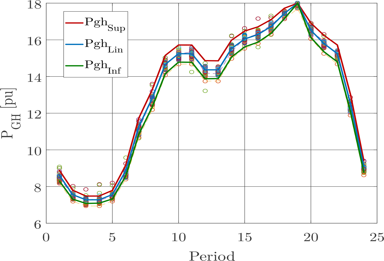
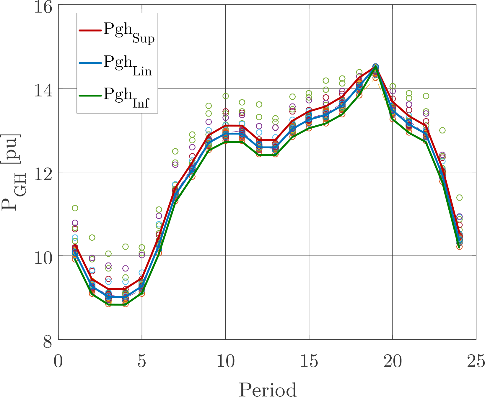
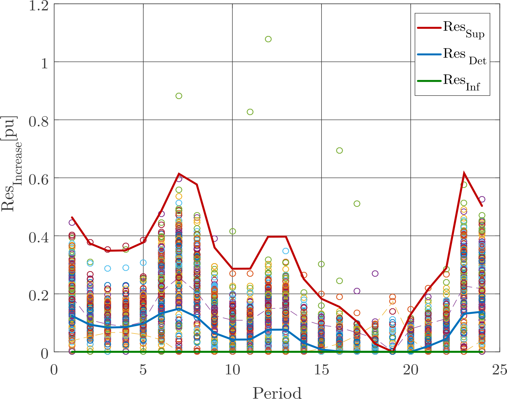
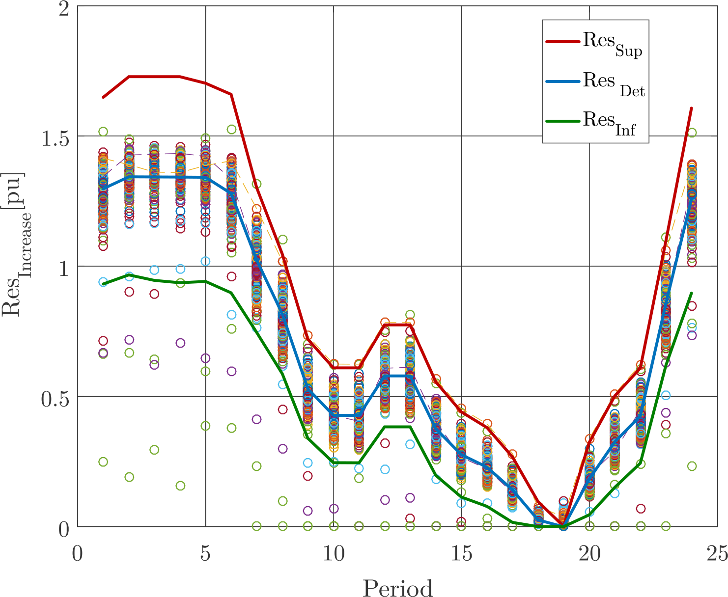
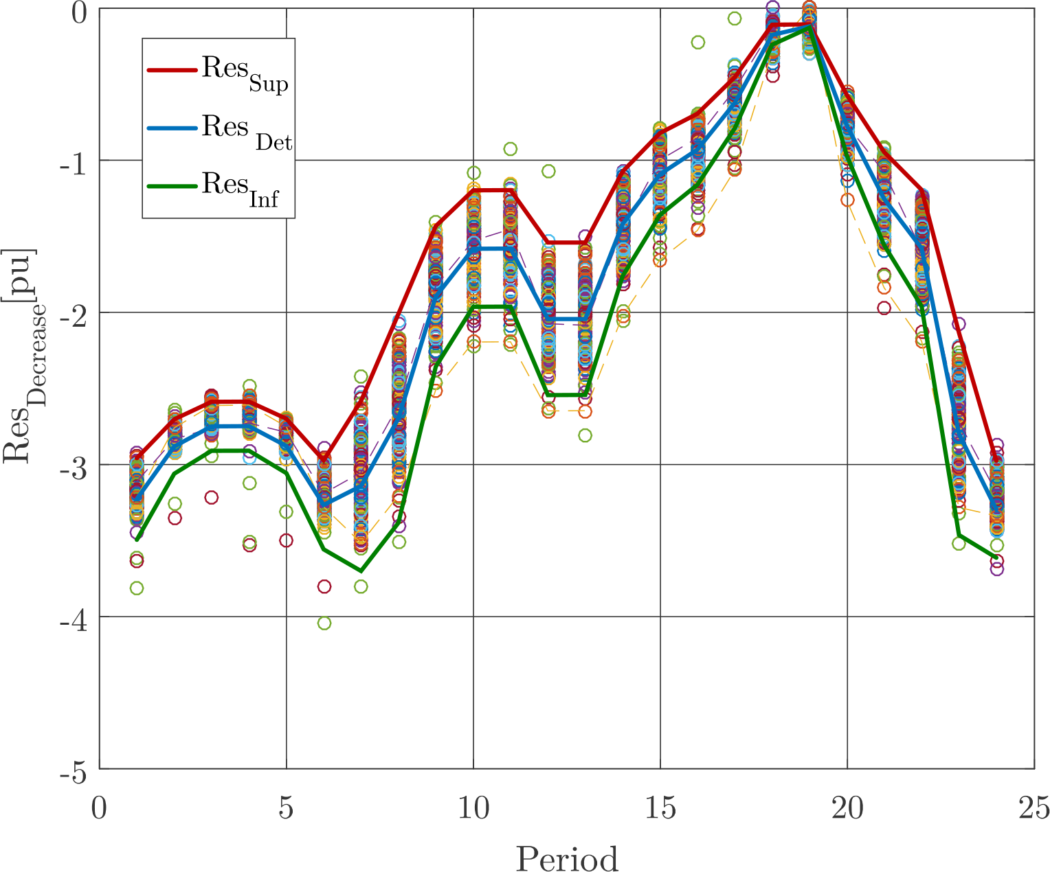
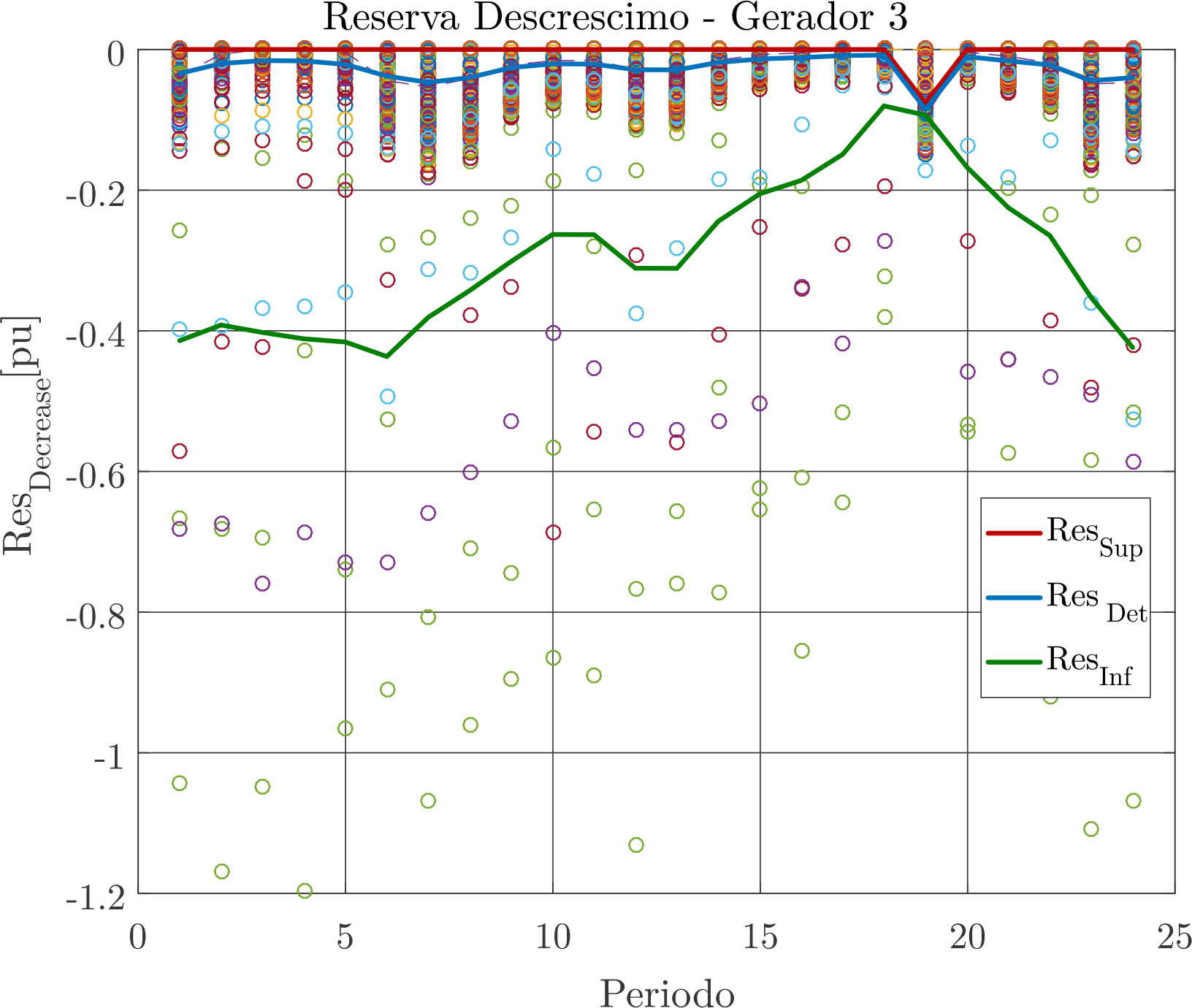
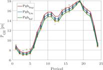
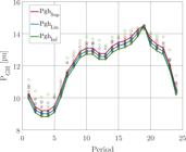
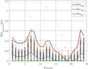
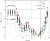
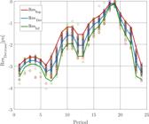
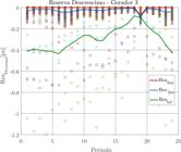
The results are presented in the form of hourly graphs that include: (i) active power dispatch values of the generators 1 and 3 obtained by the MMOPF, designated by the subscript lin, and the superior and inferior intervals obtained by the IMMOPF, designated by the subscripts sup and inf (Figure 1 and 2); (ii) values of active power SR of increase of the two generators obtained by the MMOPF, and their superior and inferior intervals, obtained by the IMMOPF (Figure 3 and 4); and (iii) values of the active power SR of decrease for the two generators obtained by the MMOPF, and their superior and inferior intervals, as obtained by the IMMOPF (Figure 5 and 6).

Figure 1
Power dispatch results for generator 1

Figure 2
Power dispatch results for generator 3

Figure 3
Increase in reserve for generator 1

Figure 4
Increase in reserve for generator 3.

Figure 5
Decrease in reserve for generator 1

Figure 6
Decrease in reserve for generator 3.

Validation of Results

To validate the IMMOPF results, clouds of random values were generated through 200 simulations using the MMOPF, where each element of the load vector (Pd) was incremented with a uniform probability distribution margin equal to ±2%. The cloud values are shown in Figures 1 to 6. It can be observed that the intervals calculated by the interval method create an envelope around the random cloud in each figure.

Tables 3 to 5 present the values related to generation (Pgh), increase in reserve ($Re{s}_{incresae}$) and decrease in reserve ($Re{s}_{decrease}$), respectively, for generators 1 and 3, for periods of light, medium and heavy load. All three tables present the interval values obtained by IMMOPF, the cloud limit values within the interval range [³⁸], the mean and standard deviation of the cloud values, and the relative difference between the limits obtained via IM and via random cloud.

Table 3
Comparison of Pghs

Method	Period	$Pgh\_1_{sup}$ [pu]	Dif %	$Pgh\_3_{sup}$ [pu]	Dif %	$Pgh\_1_{inf}$ [pu]	Dif %	$Pgh\_3_{inf}$ [pu]	Dif %
IMMOPF	5	7.79	1.54	9.47	0.32	7.32	0.13	9.11	0.44
Random		7.67		9.44		7.33		9.15
Mean		7.73 0.085		9.46 0.020		7.33 0.007		9.13 0.028
Std Dev.
IMMOPF	12	14.87	0.95	12.77	0.23	13.88	0.65	8.63	1.05
Random		14.73		12.74		13.97		8.54
Mean		14.80 0.09		12.76 0.020		13.93 0.064		8.58 0.036
Std Dev.
IMMOPF	20	16.91	0.35	13.70	0.73	16.12	0.75	13.28	0.07
Random		16.85		13.60		16.24		13.27
Mean		16.88 0.042		13.65 0.070		16.18 0.085		13.27 0.007
Std Dev

Table 4
Comparison of Reserves of Increase values

Method	Period			$Res{1}_{increase}sup$	Dif %			$Res{3}_{increase}sup$	Dif %			$Res{1}_{increase}inf$	Dif %			$Res{3}_{increase}sup$		Dif %
				[pu]				[pu]				[pu]				[pu]
MMOPF		5	0.380			2.64	1.700			11.7	0.0			0	0.940		8.51
Random			0.370				1.500				0.0				1.020
Mean			0.375 0.0071				1.600 0.140				0.0 0.0				0.980 0.057
Std Dev
MMOPF		12	0.390			17.9	0.770			1.29	0.0			0	0.380		13.16
Random			0.320				0.760				0.0				0.430
Mean			0.360 0.050				0.765 0.0071				0.0 0.0				0.410 0.035
Std Dev
MMOPF		20	0.130			8.33	0.300			6.67	0.0			0	0.050		0
Random			0.120				0.320				0.0				0.050
Mean			0.125 0.0071				0.310 0.014				0.0 0.0				0.050 0.000
Std Dev

From Table 3 (generation values), Table 4 (increase in reserve values) and Table 5 (decrease in reserve values), it can be observed that the all the standard deviation values have a low dispersion on the order of 10^-2 pu.

Table 5
Comparison of Reserves of Decrease values

Method	Period			$Res{1}_{decres}\_sup$	Dif %			$Res{3}_{decres}\_sup$	Dif %			$Res{1}_{decres}\_inf$		Dif %		$Res{3}_{decres}\_inf$		Dif %
				[pu]				[pu]				[pu]				[pu]
MMOPF		5	-2.70			0.37	0.0			0	-3.01		1.33		-0.41		9.75
Random			-2.71				0.0				-2.962				-0.37
Mean			-2.71 0.007				0.0 0.0				-2.99 0.029				-0.39 0.028
Std Dev
MMOPF		12	-1.54			3.25	0.0			0	-2.50		2.80		-0.32		9.37
Random			-1.59				0.0				-2.43				-0.29
Mean			-1.57 0.035				0.0 0.0				-2.47				-0.31 0.021
Std Dev											0.049
MMOPF		20	-0.57			1.75	0.0			0	-0.97		1.03		-0.16		18.75
Random			-0.58				0.0				-0.96				-0.13
Mean			-0.58 0.007				0.0 0.0				-0.97 0.007				-0.15 0.021
Std Dev

The relative differences between intervals obtained via IM and via load values are as follows: (i) less than 1.54 % (generation values), (ii) percentages varying from 0% to 17.9% (increase in reserve), and (iii) percentages varying from 0% to 18.75% (decrease in reserve). In most results, there is an alignment between the values obtained by the deterministic IM technique and via the probabilistic technique that involved exhaustive simulations.

To complement the results, the average percentage of random cloud values falling in the range generated by the proposed method (IMMOPF) was evaluated. It can be seen from Table 6 that most of the cloud values fall within the superior and inferior intervals obtained by the IMMOPF method.

Table 6
Percentage of cloud included in the IMMOPF range

Variable	Generator 1	Generator 3
Phg	95.22%	95.33%
$Re{s}_{incres}$	99.74%	98.12%
$Re{s}_{decres}$	92.99%	96.00%

Table 7 shows the average accommodation index (A) for the generation values, and the increase and decrease in reserve values for light, medium and heavy load periods (hours 5, 12 and 20, respectively). The details of the calculation method can be seen in [³⁸], and involve calculating the ratio between the diameters of the interval created by the reference method (cloud values) and the proposed method (IMMOPF). The closer this value is to 100%, the better the result, with 100% indicating a perfect overlap between the intervals of the proposed methods. Results of above 30% are considered satisfactory [³¹,³⁸].

Table 7
Average accommodation index

Period	A - Pgh	A - $Re{s}_{Increase}$	A - $Re{s}_{decrease}$
5	78.01%	73.17%	74.38%
12	81.01%	72.41%	62.81%
20	79.20%	83.14%	69.06%

Table 8 shows the specific accommodation indexes for the three variables, for each of the generators. We can see that most of the values obtained by the cloud method have an average accommodation degree, all above 62%, indicating a good approximation of the proposed method to the results obtained from the validation method.

Table 8
Accommodation index (A) of generators 1 and 3 for each load levels considered

Period	$A\left(Pgh1\right)$	$A\left(Pgh3\right)$	$A(Res{1}_{increase}$)	$A\left(Res{3}_{increase}\right)$	$A(Res1{decrease}_{}$)	$A\left(Res3{decrease}_{}\right)$
5	71.66%	94.51%	77.91%	61.79%	73.39%	85.10%
12	76.93%	85.94%	79.76%	83.53%	84.30%	93.66%
20	77.99%	77.87%	90.39%	88.01%	98.57%	81.15%

Finally, the execution time of the proposed method was evaluated. The system configuration used for this was a Ryzen 7 3800X CPU, 16 GB DDR4. It took 59 hours to obtain the cloud of 200 values, while it took only five hours to obtain the range via IMMOPF. One of the reasons for simulating only 200 random values was the limitations on the hardware.

CONCLUSION

This work aimed to create a linear MMOPF to calculate and allocate the amounts of SR required to meet different scenarios involving contingencies. In addition, the model optimizes the hydraulic dispatch and monitors the operational limits of the network.

To evaluate the results, we used a 291-bus system that was equivalent to that of the state of Paraná in Brazil. In the first analysis, the results obtained from the MOPF (which incorporates the ONS rule) and the proposed MMOPF were compared. Both methods showed little divergence between the values related to the individual dispatches of each machine per period and the total amount of the reserve. However, the proposed method obtained a total allocated reserve value that was 9.8% lower than that of the MOPF, and reduced the total daily load shedding.

In addition, IM was applied through the KM to consider the uncertainty in load data (IMMOPF), thus obtaining optimal generation and reserve intervals.

As a validation method, the MMOPF was simulated 200 times, with 2% uncertainty in the loads in each of the simulations. In this way, a cloud of values was generated, which allowed for the creation of an interval and thus enabled validation of the results obtained by the IMMOPF.

Tests were performed with the 291-bus system, and the results showed good precision and uniformity, low dispersion, and performance that was about 12 times faster than the validation method.

The main contributions of this work are as follows: (i) we have calculated the amount and allocation of reserve required for a multi-period and multi-contingency analysis simultaneously, and (ii) we have obtained optimal intervals for pre-defined uncertainties using the incorporation of IM.

• Funding:
  This research received no external funding.

Acknowledgments:

This research was funded by CAPES - Brazilian Federal Agency for Support and Evaluation of Graduate Education within the Ministry of Education of Brazil.

Data Availability Statement:

Research data are only available upon request for corresponding author.

REFERENCES

• ¹ Moraes RA, Fernandes TSP, Arantes AG, Vila CU. Short-Term Scheduling of Integrated Power and Spinning Reserve of a Wind-Hydrothermal Generation System with AC Network Security Constraints. J. Control Autom. Electr. Syst. p. 29, 2017.
• ² Naversen CØ, Farahmand H, Helseth A. Procurement of spinning reserve capacity in a Hydropower dominated system through Mixed Stochastic-robust optimization. Opt. and Cont., arXiv:1903.04805, 2019.
  » https://doi.org/1903.04805
• ³ Tavares LA. [Brazilian Electricity Matrix and Future Trends]- Revista Científica Multidisciplinar - ISSN 2675-6218. 2023;4(5):e453135.
• ⁴ Jamshidi S, Bagheri H, Hasanvand S, Hassanzadeh ME, Rohani A. Impact of spinning reserve on frequency control in a hybrid power plant including renewable energy. J. Green Energy Res. Innov. 2024.
• ⁵ ONS (Operador Nacional do Sistema). [Operation Procedures Manual]. 2022.
• ⁶ Wang Z, Alvarado FL. Interval arithmetic in power flow analysis. IEEE Trans. Power Syst. 1992;7(3):1341-9.
• ⁷ Pereira LES, da Costa VM, Rosa ALS. Interval arithmetic in current injection power flow analysis. Int. J. Electr. Power Energy Syst. 2012;43(1):1106-13.
• ⁸ Costa AL. [Joint optimal allocation of energy and operating reserves based on dynamic optimal power flow] [doctoral thesis]. Florianopolis: Federal University of Santa Catarina, Brazil, 2004.
• ⁹ Shayesteh E, Yousefi A, Parsa Moghaddam M. A probabilistic risk-based approach for spinning reserve provision using day-ahead demand response program. Energ. 2010;35(5):1908-15.
• ¹⁰ Partovi F, Nikzad M, Mozafari B, Ranjbar AM. A stochastic security approach to energy and spinning reserve scheduling considering demand response program. Energ. 2011;36(5):3130-7.
• ¹¹ Sahebi MMR, Hosseini SH. Stochastic security constrained unit commitment incorporating demand side reserve. Int. J. Electr. Power Energy Syst. 2014; 56:175-84.
• ¹² Amirahmadi M, Akbari Foroud A. Stochastic multi-objective programming for simultaneous clearing of energy and spinning reserve markets considering reliability preferences of customers. Int. J. Electr. Power Energy Syst. 2013; 53:691-703.
• ¹³ Liu G, Tomsovic K. Quantifying spinning reserve in systems with significant wind power penetration. IEEE Trans. Power Syst. 2012; 27(4):2385-93.
• ¹⁴ Reddy SS, Panigrahi BK, Kundu R, Mukherjee R, Debchoudhury S. Energy and spinning reserve scheduling for a wind-thermal power system using CMA-ES with mean learning technique. Int. J. Electr. Power Energy Syst. 2013; 53:113-22.
• ¹⁵ Chen C-L, Chen Z-Y, Lee T-Y. Multi-area economic generation and reserve dispatch considering large-scale integration of wind power. Int. J. Electr. Power Energy Syst. 2014; 55:171-8.
• ¹⁶ Fernandez-Blanco R, Dvorkin Y, Ortega-Vazquez MA. Probabilistic security-constrained unit commitment with generation and transmission contingencies. IEEE Trans. Power Syst. 2017; 32(1):228-39.
• ¹⁷ Mogo JB, Kamwa I. Improved deterministic reserve allocation method for multi-area unit scheduling and dispatch under wind uncertainty. J. Mod. Power Syst. Clean Energy. 2019; 7(5):1142-54.
• ¹⁸ Jung C-M, Reddy SS. Optimal wind-thermal coordination scheduling considering reserve requirement. Int J. Math. Eng. Manag Sci. 2019; 5(1):108-19.
• ¹⁹ Sun B, Dai W, Zhang D, Goh HH, Zhao J, Shi B, et al. An effective spinning reserve allocation method considering operational reliability with multi-uncertainties. IEEE Trans. Power Syst. 2024; 39(1):1568-81.
• ²⁰ Fan N, Chen R, Watson J. N-1-1 contingency-constrained optimal power flow by interdiction methods. In: 2012 IEEE PES General Meeting. IEEE; 2012.
• ²¹ Zheng JH, Chen JJ, Wu QH, Jing ZX. Reliability constrained unit commitment with combined hydro and thermal generation embedded using self-learning group search optimizer. Energ. 2015; 81:245-54.
• ²² Banshwar A, Sharma NK, Sood YR, Shrivastava R. Market based procurement of energy and ancillary services from Renewable Energy Sources in deregulated environment. Renew. Energ. 2017; 101:1390-400.
• ²³ Darvish H, Darvishi A, Hejazi H. Integration of demand side management in security constrained energy and reserve market. In: 2015 IEEE Power & Energy Society Innovative Smart Grid Technologies Conference (ISGT). IEEE; 2015.
• ²⁴ Damodaran S, Sunil Kumar T. Hydro-thermal-wind generation scheduling considering economic and environmental factors using heuristic algorithms. Energies. 2018; 11(2):353.
• ²⁵ Yang C, Tian K, Gao X. Supply chain resilience: Measure, risk assessment and strategies. Fund. Res. 2023.
• ²⁶ Mori H, Yuihara A. Calculation of multiple power flow solutions with the Krawczyk method. In: ISCAS’99 Proceedings of the 1999 IEEE International Symposium on Circuits and Systems VLSI (Cat No99CH36349). IEEE; 2003.
• ²⁷ Pereira LES. [Generalized methodologies for solving interval power flow considering uncertain data]. [Juiz de Fora - MG]: Federal University of Juiz de Fora, Brazil; 12-Jun-2015.
• ²⁸ Del Monego A, Fernandes TSP: Optimal Power Flow Analysis with Interval Mathematics -the Krawczyk Method. The 12th Latin-American Congress on Electricity Generation and Transmission - CLAGTEE 2017.
• ²⁹ Lu F, Du P, Liu H, Liu F. Affine arithmetic-based power flow algorithm considering uncertainty for hybrid AC/DC grids incorporating VSCs. IET Gener. Transm. Distrib. 2019; 13(10):1856-64.
• ³⁰ Borba RA. [Interval mathematics applied to multi-period and three-phase optimal power flow]. [Curitiba]: Federal University of Paraná, Brazil; 2020.
• ³¹ Rodrigues Junior HM, Melo ID, Nepomuceno EG. An interval power flow for unbalanced distribution systems based on the Three-Phase Current Injection Method. Int. J. Electr. Power Energy Syst. 2022; 139(107921).
• ³² Moore RE, Kearfott RB, Cloud MJ. Introduction to Interval Analysis. Cambridge University Press; 2009.
• ³³ Gwaltney CR, Lin Y, Simoni LD, Stadtherr MA. Interval methods for non-linear equation solving applications. In: Handbook of Granular Computing. Chichester, UK: John Wiley & Sons, Ltd; 2008. p. 81-96
• ³⁴ De Vargas RR, De Farias CM, Barboza LV, Dimuro GP. [Data Uncertainty in Power Flow: An Approach with the Interval Mathematics of C-XSC]. TEMA Tend. Mat. Ap.l Comput. [Internet]. 2008;9(3).
• ³⁵ Krawczyk R, [Newton algorithms for determining zeros with error bounds], Comp., 1969. vol. 4, no. 3, p. 187-201.
• ³⁶ Wu H, Zhou L, Wan Y, Liu Q, Zhou S. A mixed uncertainty power flow algorithm-based centralized photovoltaic (PV) cluster. Energies. 2019;12(20):4008.
• ³⁷ Fernandes TSP, Lenzi JR, Mikilita MA, Load Shedding Strategies Using Optimal Load Flow with Relaxation of Restrictions. IEEE Trans. Power Syst.; 2008. vol. 23, no. 2, p. 712-18.
• ³⁸ Leng S, Liu K, Ran X, Chen S, Zhang X. An affine arithmetic-based model of interval power flow with the correlated uncertainties in distribution system. IEEE Access [Internet]. 2020; 8:60293-304.

• Editor-in-Chief:
  Alexandre Rasi Aoki

• Associate Editor:
  Alexandre Rasi Aoki

Publication Dates

• Publication in this collection
  14 July 2025
• Date of issue
  2025

History

• Received
  10 Nov 2024
• Accepted
  28 Apr 2025