Calculation of a quasi-geoid model based on the scalar-free solution of the Geodetic Boundary Value Problem (GBVP) with numerical integration of Stokes integrals within the Colorado Experiment

Abstract:

This paper presents the approach proposed by UFPR for calculating a quasi-geoid model within the Colorado Experiment (CE) based on the scalar-free solution of the Geodetic Boundary Value Problem (GBVP), using Molodensky series and numerical solutions of Stokes integrals. The study area covers part of the state of Colorado, USA, where fourteen different research groups sought to model the Earth’s gravity field with centimeter precision. The model was calculated from residual Molodensky gravity anomaly values, calculated using available ground and airborne data, using the Remove-Compute-Restore (RCR) technique. Tests were conducted to identify the optimal Wong and Gore (WG) modification degree and cap size to best fit the model to the GSVS17 reference data. Analysis of the results revealed that the model had a standard deviation of 2.7 cm, an RMSE of 86.4 cm, and lower variability compared to solutions from the other 12 institutions. It was also found that the solution is significantly influenced by changes in the Wong and Gore modification degree. The study concludes that the solution proposed here is an effective alternative for calculating quasi-geoid models and for point-based geopotential modeling within the scope of International Height Reference Frame (IHRF) implementation, even in areas with complex topography.

Keywords:
Colorado Experiment; IHRS; IHRF; quasi-geoid; scalar-free GBVP

1. Introduction

The definition of a global height reference system is one of the major challenges in modern geodesy, aiming to overcome limitations of traditional systems. These systems, historically based on Mean Sea Level (MSL) observations, present discrepancies that hinder the integration and sharing of data between different countries (Sánchez et al., 2016; Sánchez et al., 2021). To address this issue, the International Association of Geodesy (IAG), in July 2015, through Resolution No. 1, established the parameters for the definition and realization of the International Height Reference System (IHRS). This system adopts a unified reference based on a conventional value of the Earth’s gravity potential, ensuring that all regional height systems are referred to the same geopotential reference surface (Drewes et al., 2016). For the realization of this system, the accurate determination of the Earth’s gravity field at the centimeter level is one of the fundamental requirements for the implementation of the IHRF (Sánchez et al., 2021).

In this context, methodological comparison experiments become essential to assess whether current strategies for solving the GBVP are capable of meeting the stringent accuracy requirements imposed by the IHRF. Within this framework, the Colorado Experiment (CE) represents a significant contribution from 14 research groups, which between 2018 and 2020 dedicated themselves to calculate and determine Earth’s gravity field models with an accuracy of 1 cm. The main objective was to estimate and compare different methodologies to achieve this accuracy using a single dataset to obtain results as close as possible to this accuracy (Sánchez et al., 2018).

The experiment took place in the state of Colorado, USA, using data provided by the National Geodetic Survey (NGS). The experiment covered an area measuring approximately 730 km × 560 km, which presents challenging geographic characteristics, with altitudes ranging from 932 m to 4,385 m. The dataset used by all groups included ground-based and airborne gravity data, global geopotential models (GGM), a digital elevation model (DEM), and historical GNSS survey measurements based on level references. For the final validation of the developed models, an independent dataset was made available, originated from a recent leveling line.

The methodological approaches adopted by the participating groups in the Colorado Experiment (CE) were based on different formulations of the Geodetic Boundary Value Problem (GBVP). Most groups, such as Aristotle University of Thessaloniki (AUTh), Technical University of Denmark (DTU), New Technologies for the Information Society (NTIS-GEOF), and Politecnico di Milano (POLIMI), adopted the Molodensky formulation within the Remove-Compute-Restore (RCR) framework, combining global geopotential models (GGM), terrain corrections and residual gravity anomalies (Wang et al., 2021; Grigoriadis et al., 2021; Isik et al., 2021; Varga et al., 2021). These approaches commonly relied on Fast Fourier Transform (FFT) techniques to solve Stokes integrals. In contrast, a smaller number of groups adopted Stokes-based solutions with least-squares modification techniques (e.g., LSM Stokes) or alternative collocation-based approaches (Claessens and Filmer, 2020; Liu et al., 2020).

Additionally, several studies focused on the integration of airborne gravity data using least-squares collocation (LSC) and radial basis functions (SRBF), highlighting the importance of combining heterogeneous datasets for high-resolution quasi-geoid modelling (Grigoriadis et al., 2021; Liu et al., 2020). A comprehensive overview of the methodological choices, parameter settings and reference models adopted by each group is provided in Wang et al. (2021), which serves as a benchmark for comparative analysis.

The results obtained within the CE showed a significant correlation between terrain effects and the proposed approaches. Differences in the determination of the disturbance potential (T), using the same data and different gravity field modeling strategies, resulted in solutions with standard deviations between 0.009 m and 0.023 m relative to the mean value (Sánchez et al., 2024). The individual RMS value of the solutions ranged from 1.6 cm to 5.3 cm, with an average of 2.0 cm, indicating that no approach achieved the required accuracy (Wang et al., 2021).

Following the Colorado Experiment, several studies have been conducted with the objective of proposing and validating alternative methodologies for regional gravity field modelling. Among these, Padilha et al. (2026) investigated a quasi-geoid solution based on a fixed GBVP formulation using the Brovar series, contributing to the ongoing development of methodologies within the CE framework.

To contribute to the CE and to the state-of-the-art for the calculation of quasi-geoid models and geopotential number values within the International Height Reference Frame (IHRF), this work proposes and evaluates an alternative solution. It was based on the scalar-free solution of the Geodetic Boundary Value Problem (GBVP), using the Molodensky series (Molodensky et al., 1960), modified by Wong and Gore (Wong and Gore (1969) - WG), but with the numerical integration of Stokes integrals. The results obtained were evaluated in absolute terms using the GSVS17 profile data and compared with 12 CE solutions available from the International Service for the Geoid (ISG). The participating institutions, methodological approaches and corresponding references are summarized in Table 1. This analysis is particularly relevant to assess the potential of the solution for geopotential modeling at future International Height Reference Frame (IHRF) stations and for the calculation of quasi-geoid models in other regions.

This paper is structured as follows: Section 2 describes the study area and the dataset, detailing the terrestrial and airborne gravity data sources, the digital elevation model (DEM), and the GSVS17 validation profile. Section 3 presents the theoretical background and methodology, focusing on the Remove-Compute-Restore (RCR) procedure, the application of the scalar-free solution of the GBVP using the Molodensky series, and the implementation of numerical integration with the Wong and Gore modification. Section 4 presents the results and discussion, including the statistical analysis of the optimized model, the absolute and relative validation, and the comparison with the 12 reference solutions from the Colorado Experiment. Finally, Section 5 summarizes the conclusions and outlines perspectives for future research on the implementation of the IHRF.

2. Area under study: dataset and preprocessing

The Colorado Experiment encompasses an area between latitudes 35°N and 40°N and longitudes 110°W and 102°W in Colorado, USA. It contains an abundance of geodetic data from various sources in a region with considerable topographic variation, making the objective quite complex. A recent GNSS-tracked leveling network and both terrestrial and airborne gravity data are available in the region. It is worth noting that the solutions calculated in this work used only a combination of both types of gravity data, since within the CE framework, the combination yielded better results.

Figure 1:
CE region. In yellow (terrestrial gravimetry data), Perpendicular lines in blue (airborne gravimetry data), Blue rectangle (area where the quasi-geoid modeling was done).

The gravity data provided by NGS correspond to 59,303 points available in separate columns as follows: latitude (°), longitude (°), orthometric height above MSL (m), gravity g (mGal), survey ID, and year. The latitude and longitude values are referenced to the North American Datum of 1983 (NAD83) as defined by the National Geodetic Survey (NGS, 2023), which was considered compatible with International Terrestrial Reference Frame/International GNSS Service (ITRF/IGS08) (Altamimi et al., 2011), and to the tide-free concept, as were the gravity values. The orthometric altitudes were considered referenced to NAVD88, since all were dimensioned from topographic maps or barometric altitudes (AHLGREN, 2024 - personal communication). Consequently, to obtain the ellipsoidal altitude h of these points, the hybrid geoid model GEOID18 (Ahlgren et al., 2020) was used. Ground gravity data are presented in yellow in Figure 1.

Available airborne gravity data come from the Grav-D Project (GRAV-D Science Team, 2018) based on the MS05 block, previously filtered and resampled to 1 Hz. The set contains 283,716 points with columns divided into: block, line, time, (°), (°), ellipsoidal height (m), and gravity (mGal). Geodetic coordinates are in the IGS08 system. All values are tide-free. Airborne gravity data, arranged in blue lines, are presented in Figure 1.

The DEM available for the project was SRTM v4.1 (Jarvis et al., 2008). However, for modeling the short wavelengths of the gravity field, within the RCR technique, the solution presented here followed the strategy of some groups that used Earth2014 (Rexer et al., 2016) and ERTM2160 (Hirt et al., 2014) models together, as AUTh, Deutsches Geodätisches Forschungsinstitut (DGFI), Institute for Astronomical and Physical Geodesy (IAPG) and POLIMI (Grigoriadis et al., 2021; Liu et al., 2020; Willberg et al., 2020), both based on the same SRTM data.

Data preprocessing began with the detection and elimination of redundant ground-based gravity data. Points with the same coordinates were removed from the dataset. A total of 1,090 points were identified and removed. Regarding the airborne gravity data, the abundance of data available at a rate of 1 Hz makes the values of nearby points highly correlated, in addition to increasing the computational effort and suggesting a non-significant contribution (Liu et al., 2020). Therefore, the data were resampled to 0.2 Hz, totaling 56,769 points.

To validate the calculated models, data from 222 GNSS-leveling benchmarks, meticulously materialized in the Geoid Slope Validation Survey 2017 (GSVS17) project, were made available. The leveling closure error was 0.7 , and included GNSS measurements, relative and absolute gravimetry, and vertical deflection (Van Westrum et al., 2021). The points of the GSVS17 profile are shown in red in Figure 1.

3. Methodology

Three steps were followed to calculate the model: i) obtain and pre-process the data; ii) calculate the optimized model, applying the RCR technique and numerical integration of Stokes’ integrals, iteratively to find the degree of modification of WG and ideal cap size; and iii) the absolute statistical evaluation of the optimized model. This procedure is shown in Figure 2.

Figure 2:
Scheme for the quasi-geoid model calculation.

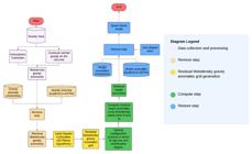
Table 1 summarizes the Colorado Experiment (CE) solutions considered in this study, including the participating institutions, abbreviations and corresponding references.

Table 1:
Overview of the Colorado Experiment (CE) solutions used for comparison in this study, including the participating institutions, computation methodologies and corresponding references.

Computation method	Authors	Institutions
1D FFT with Wong-Gore modification of the Stokes kernel	Grigoriadis et al., 2021	Aristotle University of Thessaloniki (AUTh)
1D FFT with Wong-Gore modification of the Stokes kernel	Claessens and Filmer, 2019	Curtin University (Curtin)
Spherical FFT with Wong-Gore modification of the Stokes kernel	Forsberg, 1987	Technical University of Denmark (DTU)
FFT with degree-banded modification of the Stokes kernel	Huang and Véronneau, 2013	Canadian Geodetic Survey (CGS)
Windowed Least-Squares Collocation	Barzaghi et al., 2020	Politecnico di Milano (POLIMI)
Residual Least-Squares Collocation	Willberg et al., 2020	Institute for Astronomical and Physical Geodesy (IAPG)
Spherical Radial Basis Functions	Liu et al., 2020	Deutsches Geodätisches Forschungsinstitut (DGFI)
Least Squares modification of Stokes integral	Ågren et al., 2009	University of Gävle (KTH)
Least Squares modification of Stokes integral	Varga et al., 2021	New Technologies for the Information Society (NTIS-GEOF)
Least Squares modification of Stokes integral	Işık et al., 2021	Istanbul Technical University (ITU-GRG)
Modified Stokes integral Meissel-Molodensky modified kernel	Matsuo and Forsberg, 2021	Geospatial Information Authority of Japan (GSI)
Spectral combination approach	Jiang et al., 2020	Chinese Academy of Surveying and Mapping (CASM)
Spherical harmonic analysis scheme with Wong-Gore modification of the Stokes kernel	Wang et al., 2020	US National Geodetic Survey (NGS)

3.1 Remove step

The quasi-geoid model was calculated based on the scalar-free solution of the GBVP, using Molodensky’s shrinking method (Molodensky et al., 1960), adapted to the Remove-Compute-Restore technique. The first step was to obtain the Molodensky gravity anomalies (∆g _M ), given by the differences between the gravity observed at point P(g _P ) on the Earth’s surface and the normal gravity at point Q (γ _Q ), which is the projection of point along the plumb line onto the telluroid (Eq. (01)). Furthermore, the atmospheric correction was applied, which was calculated according to Wenzel (1985), given the fact that GRS80 does not include it.

$\Delta g_M=g_p-{\gamma }_Q+C_{ATM}$ (01)

where:

${\gamma }_Q=\gamma \left[1-2\left(1+f+m-2fse{n}^2\phi \right)\frac{H^N}{a}+3{\left(\frac{H^N}{a}\right)}^2\right]$ (02)

In Eq. (02), f is the geometrical flattening of the ellipsoid; m is the ratio of centrifugal and gravity acceleration at its equator; φ is the geodetic latitude; and is the equatorial radius. Following the conventions for the CE, the reference ellipsoid used was the Geodetic Reference System of 1980 (GRS80) (Moritz, 2000). Thus, the values of normal gravity on the ellipsoid (γ) were calculated using the Gravity Formula 1980, which corresponds to the Somigliana’s formula adapted to the GRS80 reference system (Moritz, 2000).

In the case of terrestrial data, the normal altitude values H _N presented in Eq. (02) were calculated from the orthometric altitude values H, using the relationship indicated in Eq. (03), where ∆g _B is the Bouguer anomaly, given by Eq. (04), and $\overline{\gamma }$ is the mean normal gravity along the normal plumb line, given by Eq. (05). Further details on the equations can be found in Hofmann-Wellenhof and Moritz (2006).

$H^N=H+H\frac{{∆g}_B}{\overline{\gamma }}$ (03)

${∆g}_B=g-\gamma +0.1967H$ (04)

$\overline{\gamma }=\gamma \left[1-\left(1+f+m-2fse{n}^2\phi \right)\frac{H^2}{a}+{\left(\frac{H}{a}\right)}^2\right]$ (05)

Regarding the airborne data, the values of normal heights were calculated by subtracting from the ellipsoidal heights h height anomaly values obtained from the GGM XGM2019e (Zingerle et al., 2020) up to degree and order (D/O) 2190 (ζ _XGM2019 ):

$H^N=h-{\zeta }_{XGM2019}$ (06)

In the remove step, the objective is to obtain a smooth field with mean and standard deviation values as close to zero as possible. The gravity anomaly values for long, medium, short, and very short wavelengths are removed from the ∆g _M obtained by Eq. (01), obtaining the residual Molodensky gravity anomalies ${{{\mathrm{\Delta }}_g}_M}_{res}$. The low frequencies of the gravity anomalies were computed using XGM2016 (Pail et al., 2018), as adopted in other solutions to the CE by AUTh, DTU, GSI, Istanbul Technical University (ITU), NTIS-GEOF and POLIMI (Wang et al., 2021; Grigoriadis et al., 2021; Matsuo and Forsberg, 2019; Isik et al., 2021; Varga et al., 2021). The choice of this GGM is to use the same dataset available at the time of the CE, to allow comparisons free of biases due to differences in input data.

The high frequencies of the gravity anomalies were computed via the Residual Terrain Modelling (RTM) technique (Forsberg, 1984), using a spectral approach. The spectral domain was used with the EARTH2014 (Rexer et al., 2016) and ERTM2160 (Hirt et al., 2014) topographic models in conjunction as in the AUTh, DGFI, IAPG and POLIMI solutions (Grigoriadis et al., 2021; Liu et al., 2020; Willberg et al., 2020; Varga et al., 2021). The EARTH2014 model allowed a spherical harmonic expansion up to degree and order (D/O) 2160, and the ERTM2160 extends the expansion to about 81000 (Hirt et al., 2014).

For the values obtained from XGM2016, three D/O thresholds were considered, i.e., 300, 500, and 719, referred to as transition D/O. This was done to analyze the influence of different truncation levels of the GGM on the accuracy of the computed quasi-geoid model. In consequence, in the RTM computations for terrestrial data, the EARTH2014 model was used from D/O 301, 501 and 720 up to D/O 2159, while the ERTM2160 model was used from D/O 2160 up to approximately 81,000. In the case of the airborne data, the RTM gravity anomalies were computed using only the EARTH2014 model up to D/O 2160, since the very high-frequency components are not significant due to the high flight altitude (Willberg et al., 2020; Grigoriadis et al., 2021). Thus, for the removals, we have:

$\Delta {g_M}_{{res}_{terrestrial}}=\Delta g_{M_{terrestrial}}-\Delta {g_M}_{GGM}-\left(\Delta {g_M}_{{RTM}_{EARTH2014}}+\Delta {g_M}_{{RTM}_{ERTM2160}}\right)$ (07)

$\Delta {g_M}_{{res}_{airborne}}=\Delta g_{M_{airborne}}-\Delta {g_M}_{GGM}-\left(\Delta {g_M}_{{RTM}_{EARTH2014}}\right)$ (08)

where ${{{\mathrm{\Delta }g}_M}_{res}}_{terrestrial}$ and ${{{\mathrm{\Delta }g}_M}_{res}}_{airborne}$ denote the residual Molodensky gravity anomalies for terrestrial and airborne data, respectively. ${{{\mathrm{\Delta }g}_M}_{res}}_{terrestrial}$ and ${{{\mathrm{\Delta }g}_M}_{res}}_{airborne}$ represent the Molodensky gravity anomalies derived from terrestrial and airborne observations. $\Delta {g_M}_{GGM}$ are the gravity anomalies computed using XGM2016 at the selected transition D/O. $\Delta {g_M}_{{RTM}_{EARTH2014}}$ and $\Delta {g_M}_{{RTM}_{ERTM2160}}$ denote the RTM gravity anomaly from EARTH2014 and ERTM2160 models at the corresponding D/O.

The long-wavelength component derived from XGM2019 was computed using the International Centre for Global Earth Models (ICGEM) service (Ince et al., 2019), including the zero-degree term, up to the selected maximum degree and order (D/O). The high-frequency component was obtained using the RTM approach, computed via the ICGEM service using the EARTH2014 topographic model.

After obtaining the terrestrial and airborne $\Delta {g_M}_{res}$ values for each configuration and transition D/O, the residual gravity anomaly grids were computed, using both terrestrial and airborne datasets. For this purpose, the 3D least squares collocation method (3D LSC) was used, utilizing the planar logarithmic covariance function given in Eq. (09) (Forsberg, 1987). This is widely used in applications where combined ground and airborne data are available (see, for example, Tscherning et al., 1998). In this case, downward continuation of the airborne residual gravity anomaly values is performed simultaneously with interpolation to generate the regular grid.

$C\left(\mathrm{\Delta }{g_{res}^T}_1,\mathrm{\Delta }{g_{res}^T}_2\right)=f\sum _{i=0}^3{\mathit{a}}_i\log \left[D+iT+\sqrt{s^2+{\left(D+iT\right)}^2}\right]$ (09)

with

$f=\frac{C_0}{\log \left[\frac{{\left(D+T\right)}^3\left(D+3T\right)}{D{\left(D+2T\right)}^3}\right]}$ (10)

where $\mathrm{\Delta }{g_{res}^T}_1$ and $\mathrm{\Delta }{g_{res}^T}_2$ are the residual Molodensky gravity anomalies at any two points, separated by a planar distance s. a_i = [1, -3, 3, -1] are weight factors. F is a scaling factor. D is the depth of the Bjerhammar sphere. T is the low-frequency attenuation depth factor and C₀ is the variance of residual Molodensky gravity anomalies.

The first step is to estimate the empirical covariance function of the $\Delta {g_M}_{res}$ data that best describes the original covariance distribution of each smoothing configuration, that into account the different transition D/O of the GGM in the remove step. Then, the values of C₀, D, and T were obtained fitting the analytic planar logarithmic covariance function $C\left(\mathrm{\Delta }{g_{res}^T}_1,\mathrm{\Delta }{g_{res}^T}_2\right)$ to the empirical covariance function. For each configuration, the coefficient of determination (R²) between the empirical and fitted covariance functions was analyzed.

The empirical covariance of the residual gravity disturbances was estimated from pairs of observations as a function of their spatial separation. All pairwise distances were grouped into discrete intervals, and for each interval the average product of the corresponding residuals was computed, resulting in a set of empirical covariance values. This procedure follows the classical formulation for local covariance estimation described by Sansò and Sideris (2013). The resulting empirical covariance values were then used to adjust the logarithmic covariance model proposed by Forsberg (1987), which was subsequently employed in the 3D least-squares collocation.

Subsequently, the interpolation of airborne and ground data for the same surface and the downward continuation step occurred simultaneously to generate a 1’ x 1’ spatial resolution grid of residual gravity anomalies, which is the standard grid adopted in CE for all model submissions (Wang et al., 2021). To reduce the computational load, the computations were performed within 0.25° x 0.25° blocks with margins of 0.6° in all directions.

The interpolation surface was the Earth’s surface, defined in terms of ellipsoidal height values. The ellipsoidal heights of the regular grid points were obtained by summing up interpolated orthometric heights H extracted from the SRTM v4.1 DEM and interpolated geoid undulations N extracted from the EGM96 GGM (Lemoine et al., 1998). The computational routines for both steps were developed in MATLAB® software (MATLAB, 2022) using “griddataLSC” functions developed by McCubbine (2024), which was subsequently employed in the 3D least-squares collocation. This step allows the combination of terrestrial and airborne data, while simultaneously performing interpolation and downward continuation to generate a consistent residual gravity anomaly grid.

3.2 Compute step

In the compute step, the calculation of residual height anomalies ζ _res was performed from the regular grids of $\Delta {g_M}_{res}$. This was done using the scalar-free solution of GBVP, using the Molodensky series (Molodensky et al., 1960). In the solution proposed here, the series was truncated at the first-order term. This is because the RTM effect was considered in the remove step, which aids in the numerical convergence of the series (see, for example, Forsberg and Sideris (1989)). In this work, the contribution of the first-order term in the height anomaly (ζ ₁ ) proposed a millimeter or submillimeter contribution. Therefore, only the terms ${\zeta }_{0_{res}}$ and ${\zeta }_{1_{res}}$ of the Molodensky series were calculated, given by:

${\zeta }_{0_{res}}=\frac{R}{4\pi {\gamma }_Q}{\iint }_{\sigma }^{}{G}_0{S}^{WG}\left(\psi \right)d\sigma$ (11)

${\zeta }_{1_{res}}=\frac{R}{4\pi {\gamma }_Q}{\iint }_{\sigma }^{}{G}_1{S}^{WG}\left(\psi \right)d\sigma$ (12)

where $G_0={{{\Delta }_g}_M}_{res}$ and G ₁ is given by;

$G_1=\frac{R^2}{2\pi }{\iint }_{\sigma }^{}\frac{h-h_p}{l_0^3}\left[{{{\Delta }_g}_M}_{res}+\frac{3{\gamma }_Q}{2R}{\zeta }_{0_{res}}\right]d\sigma$ (13)

where, R is the radius of the Earth, h and h _p are the heights of the computation point and variable integration point, l ₀ is the distance between these points, and σ is the unit sphere. The theoretical basis behind the terms G ₀ and G ₁ can be seen in Hofmann-Wellenhof and Moritz (2006) and Tscherning et al. (1998). In Eqs. (10) and (11), S ^WG (ψ) is the Stokes function with the Wong and Gore modification (Wong and Gore, 1969) given by:

$S^{WG}\left(\psi \right)=S\left(\psi \right)-\sum _{n=2}^L\frac{2n+1}{n-1}{P}_n\left(\cos \psi \right)$ (14)

where ψ is the angular distance between the calculation point and the integration point, Pn(cosψ) is the Legendre polynomial of degree n, and L is the degree of modification. Therefore, the residual height anomaly is obtained from the sum of the terms presented in Eqs. (11) and (12):

${\zeta }_{res}={\zeta }_{0_{res}}+{\zeta }_{1_{res}}$ (15)

The integrals presented in Eqs. (11), (12), and (13) can be solved using different approaches. Within the context of the Colorado Experiment (CE), several institutions, e.g., AUTh, Curtin, NGS adopted the scalar-free formulation of the GBVP based on the Molodensky series with Wong and Gore modifications (Grigoriadis et al., 2021; Claessens and Filmer, 2020; Wang et al., 2020), typically solving the Stokes integrals using Fast Fourier Transform (FFT) techniques (Wang et al., 2021).

In contrast, in this study, the same theoretical framework is retained, but the Stokes integrals are evaluated through direct numerical integration using the Grid Line method (Hofmann-Wellenhof and Moritz, 2006). This provides an alternative solution strategy to the commonly used FFT-based approaches, allowing an independent assessment of the quasi-geoid modelling within the CE framework.

Additionally, the implementation was developed using vectorized routines in MATLAB, which allows the evaluation of all grid cells in a vectorized form, avoiding the need for explicit loop-based computations and improving computational efficiency. On other hand, although the use of vectorized routines allows efficient evaluation of the integrals, the approach may require a relatively high memory allocation, particularly for fine grid resolutions and large study areas.

The theory behind this solution consists of discretizing the integration area into several k compartments, in which each compartment will contain an associated mean gravity anomaly value $\overline{∆g_{M_{{res}_k}}}$. In practice, the integration area is limited to a certain integration radius (cap size) and k is defined. Furthermore, if the Stokes function is reasonably constant over bin k, it can be replaced by S ^WG (ψ _k ). Considering that the compartments can be subdivided in terms of latitude and longitude intervals, and following the superposition principle, Eq. (11) can be rewritten as:

${\zeta }_{{0_{res}}_j}=\frac{R}{4\pi {\gamma }_{j^{\text{'}}}}\sum _k\overline{∆g_{M_{{res}_k}}}{S}^{WG}\left({\psi }_k\right){\iint }_{{\lambda }_1{\phi }_1}^{{\lambda }_2{\phi }_2}cos{\phi }^{\text{'}}d{\phi }^{\text{'}}d\lambda \text{'}$ (16)

where γ _j , is the normal gravity value at point j’ which is the projection of point j along the plumb line onto the telluroid, and λ ₁ , φ ₁ and λ ₂ , φ ₂ are the geodetic coordinates of the southeast and northwest corners of compartment k, respectively. Multiplying the right-hand side of Eq. (16) by R/R and solving the integral, we have:

${\zeta }_{{0_{res}}_j}=\frac{1}{4\pi R{\gamma }_{j^{\text{'}}}}{\sum }_k{S}^{WG}\left({\psi }_k\right)\overline{∆g_{M_{{res}_k}}}{A}_k$ (17)

where:

$A_k=R^2\left(sen{\phi }_2-sen{\phi }_1\right)\left({\lambda }_2-{\lambda }_1\right)$ (18)

represents the area of the k compartment.

To calculate ζ ₁ it is necessary to discretize G ₁ term for each j compartment as ${G_1}_j$. Following the same idea as before for Eq. (13), the elements l ₀ and (h - h _p ) can be discretized into ${l_0}_k$ and (hk - hj) for each k compartment. With this, ${G_1}_j$ can be calculated by:

${G_1}_j=\frac{1}{2\pi }\sum _k^{}\frac{\left(h_k-h_j\right)}{{l_0^3}_k}\left(\overline{∆g_{M_{{res}_k}}}+\frac{3{\gamma }_Q}{2R}{\zeta }_{{0_{res}}_j}\right)A_k$ (19)

Similarly to the solution to Eq. (11), the solution to Eq. (12) is:

${\zeta }_{1_{{res}_i}}=\frac{1}{4\pi R{\gamma }_{i^{\text{'}}}}{\sum }_j{S}^{WG}\left({\psi }_j\right){G_1}_j{A}_j$ (20)

where γ _i , is the normal gravity value on the telluroid, i’ is the projection of i along the normal plumb line on the telluroid. And finally, for the i point we have:

${\zeta }_{{res}_i}={\zeta }_{0_{{res}_i}}+{\zeta }_{1_{{res}_i}}$ (21)

It is important to note that initially, a grid of k compartments is defined, which is used to derive two grids of j compartments with values of ${\zeta }_{{0_{res}}_j}$ and ${G_1}_j$. Subsequently, the grids of j compartments are used to generate the grid of i compartments with values of ${\zeta }_{1_{{res}_i}}$. The truncation of the Molodensky series constitutes an approximation. Nevertheless, according to Forsberg and Sideris (1989) when the RTM reduction is used, the Molodensky G ₁ term is generally insignificant. In our solution, since the RTM effect has been considered in the Remove step, only G ₀ and G ₁ were considered to compute the terms ${\zeta }_{0_{res}}$ and ${\zeta }_{1_{res}}$.

These procedures to obtain ζ _res were performed using an efficient algorithm of numerical integration, following the grid lines method of Hofmmann-Wellenhof and Moritz (2006) as previously described. This method is highly accurate and consistent with the vectorized computational solution of the MATLAB® software, or Python, which often provides faster performance than loop-based implementations (MathWorks, 2024; Abdalla and Ferreira, 2022).

The adopted numerical integration approach involves some approximations that should be considered. The discretization of the integration area into finite compartments assumes that the Stokes function and gravity anomaly values remain approximately constant within each cell, which may introduce discretization errors depending on the grid resolution. However, the final summation over all compartments generally provides stable and accurate results, especially when appropriate grid resolutions are adopted.

In the computation of ζ _res , different cap sizes and WG modification degrees were tested from multiple computations (parameter sweeps) to obtain an optimized quasi-geoid model, as in Foroughi et al. (2017) and Claessens and Filmer (2020). In practice, a range of different cap sizes, from 0° to 4° with a step of 0.1°, and modification degrees, from 30 to maximum transition D/O value of the GGM, with a step of 30 degrees were tested. Each solution was tested against GSVS17 GNSS-levelling data, yielding a set of differences in terms of ζ. The solution with the lowest standard deviation value of differences was considered optimal to compute the quasi-geoid model. It is important to notice that in this step, no quasi-geoid model was computed. The height anomaly was performed pointwise for the GSVS17 profile. The restore step was also performed pointwise following the same procedure indicated below.

3.3 Restore step and validation

In the restore step, the final height anomaly values (ζ) were calculated by adding the missing spectrum (Eq. (22)). For this purpose, the contributions of the GGM (ζ_GMM) and of the RTM (ζ_RTM ) effect were calculated using the same models as in the remove step, considering the tests with transition D/O 300, 500, and 719. Additionally, the zero-degree term (${\zeta }_{0_{IHRS}}$) calculated by Eq. (23) (Wang et al., 2021) was also added to have the solution referenced to the IHRS reference geopotential value W ₀ from IHRS (Sánchez et al., 2016). The first term of Eq. (23) was included in the ICGEM computations, while the second term was added during the restore step.

${\zeta }_i={\zeta }_{{res}_i}+{\zeta }_{{MGG}_i}+\left({\zeta }_{{EARTH2014}_i}+{\zeta }_{{ERTM2160}_i}\right)+{\zeta }_{{0_{IHRS}}_i}$ (22)

${\zeta }_{{0_{IHRS}}_i}=\frac{{GM}_{GGM}-{GM}_{GRS80}}{r_i{\gamma }_{i^{\text{'}}}}-\frac{W_0-U_0}{{\gamma }_{i^{\text{'}}}}$ (23)

where GM _GGM and GM _GRS80 is the Geocentric gravitational constant values, including the mass of the Earth’s atmosphere, of the GGM and GRS80 ellipsoid, respectively; W ₀ e U ₀ are the values of IHRS reference potential and GRS80 the reference potential on the ellipsoid, respectively; r _i is the geocentric radial distance of the computation point i on the Earth’s surface. The values of the constants used were those agreed for the CE and can be found in Sánchez et al. (2018) and Wang et al. (2021).

To validate the computed models, statistical analyses were performed on the differences between the calculated height anomalies and those obtained from the GSVS17 GNSS-leveling data at each profile point. The GSVS17 height anomaly values were calculated by subtracting the normal altitude values H ^N , provided by Van Westrum (2024, personal communication), from the ellipsoidal altitude values h (Eq. (24)). Based on these differences, the mean, standard deviation, maximum, minimum, and root-mean-square (RMS) values were evaluated. Since the parameter sweep process was used to obtain an optimized configuration, the quasi-geoid was modelled using this configuration.

$\zeta =h-H^N$ (24)

In addition to the absolute validation based on GNSS-levelling data (GSVS17), a relative validation was performed by comparing the obtained quasi-geoid model with the solutions from the Colorado Experiment and an additional relative validation based on baseline lengths was performed for the optimized solution, following the analysis adopted in the CE (Wang et al., 2021).

4. Results and discussion

Figure 3 shows the covariance functions fitted to the empirical covariance function with the index for the different D/O values of the residual Molodensky gravity anomaly grid. In this figure, the x-axis represents the covariance distance between two points and the y-axis represents the covariance between them. This covariance is higher for closer points and converges to zero as the distance increases, since points further apart have a lower correlation. The residual grids obtained a better index as the D/O value used for removal was larger. This may be due to the fact that when removing larger D/O values, ${{{\Delta }_g}_M}_{res}$ tends to be smaller and smoother. This result was also found by Grigoriadis et al. (2021).

It is worth noting that this index does not indicate the optimal D/O value to choose in the removal step, since larger D/O values also have larger commission errors arising from GGMs and should be tested for their standard deviation in relation to the GSVS17 profile.

Figure 3:
Empirical and adjusted covariance after the 3D LSC step (D/O 300 (A), 500 (B) and 719 (C) respectively).

The use of XGM2019 with a transition D/O of 719 have the highest R ² value, which proposes the best fit between empirical and fitted covariance models. In relation to the residual data used as input data to the generation of the residual Molodensky gravity anomaly grid, Table 2 shows the mean, standard deviation, maximum and minimum values of the residual Molodensky gravity anomalies. For the airborne dataset, the effect of increasing the transition D/O is more consistent. The D/O 719 configuration presents both the lowest mean and the lowest standard deviation, while D/O 300 shows the highest values for both statistics. This indicates that, for the airborne data, increasing the transition D/O improves not only the smoothness of the residual field but also reduces the residual bias.

For the terrestrial dataset, the behavior is slightly different. Although D/O 500 presents the smallest mean value, D/O 719 still provides the lowest standard deviation. This suggests a trade-off between residual bias and smoothness for terrestrial data. Therefore, D/O 719 can be interpreted as the configuration that produces the smoothest residual field, especially for the airborne data, while D/O 500 provides a slightly better bias reduction for the terrestrial component.

Regarding the extreme values, the airborne residual anomalies show a relatively controlled range, with minimum values varying from −25.398 mGal to −20.482 mGal and maximum values from 21.374 mGal to 32.861 mGal. In contrast, the terrestrial residual anomalies present larger minimum values, reaching approximately −229 mGal for D/O 300. These localized extreme values may be associated with the complex topography of the study area, local inconsistencies in the terrestrial gravity observations, or limitations in the residual modelling process. Nevertheless, despite these localized extreme values, the overall statistical behavior indicates a smoother residual field for the higher transition D/O configurations, particularly for the airborne dataset.

Table 2:
Mean, standard deviation, minimum and maximum of the terrestrial and airborne residual Molodensky gravity anomalies for each transition D/O configuration.

	Terrestrial			Airborne
	D/O 300	D/O 500	D/O 719	D/O 300	D/O 500	D/O 719
Mean	0.438	0.199	0.509	0.543	0.483	0.4617
Standard Deviation	10.901	8.304	6.974	6.598	4.167	3.178
Maximum	60.668	60.716	75.323	32.861	26.118	21.374
Minimum	-228.911	-218.441	-202.796	-25.398	-21.278	-20.482

Regarding the parameter sweep tests, the results are illustrated in Figure 4. For each transition D/O, combinations of cap size and WG modification degree were systematically tested, and each curve represents a fixed WG value as a function of the cap size. The optimal configuration was defined as the one yielding the smallest standard deviation of the differences with respect to the GSVS17 GNSS-leveling height anomalies. In Figure 4, the cap sizes are shown on the x-axis, while the corresponding standard deviations are presented on the y-axis. Table 3 summarizes the optimal configurations obtained for each transition D/O.

Despite the significant differences in cap size and Wong and Gore truncation degree, reaching variations of up to 1.8° and 449, respectively, the standard deviation values remain consistent at the millimeter level, with a maximum difference of 0.34 cm. This consistency suggests that the height anomaly results are primarily controlled by the long-wavelength components of the gravity field.

Considering the standard deviation relative to the mean solution of the CE models shown in Figure 4, the configuration yielding the lowest standard deviation corresponds to a WG modification degree of 180 for the transition D/O 300, and 210 for the other cases (D/O 500 and 719). The absolute minimum standard deviation is obtained for the configuration using transition D/O 719 with a cap size of 3.9°. Therefore, if the objective is to obtain a solution closer to the other CE solutions, this configuration would be the most appropriate.

However, since the objective of this study is to identify the solution that best fits the GSVS17 profile, the smallest standard deviation is obtained for the configuration using transition D/O 300, with a cap size of 0.9° and a WG modification degree of 270, resulting in a value of approximately 2.52 cm. A comparable result is obtained for the configuration using transition D/O 719, with a cap size of 2° and a WG modification degree of 719, reaching a standard deviation of 2.45 cm. The result obtained for transition D/O 719 is consistent with the smoothest residual Molodensky gravity anomalies reported in Table 2.

Although the D/O 719 configuration yielded the smallest standard deviation and proposes the smoothest residual Molodensky gravity anomaly field, the differences relative to the configuration that uses the D/O 300 solution are marginal (on the order of sub-millimeter level). Both configurations therefore provide comparable performance in terms of accuracy. Given this small difference, the configuration adopted to the quasi-geoid model uses a transition D/O of 300, cap size of 0.9° and 270 for the WG modification degree, as it requires a significantly smaller cap size and, consequently, reduces the computational effort. This choice allows maintaining a high level of accuracy while improving computational efficiency.

Figure 4:
WG and cap size modification degree tests for GSVS17 profile and average of the 12 CE solutions (From top to bottom D/O 300, 500 and 719 respectively).

Table 3:
Optimal configuration for each transition D/O value, based on the discrepancies with respect to the GSVS17 GNSS-leveling height anomalies.

Parameter	D/O 300	D/O 500	D/O 719
Cap size	0.9°	2.7°	2.0°
WG	270	330	719
Standard deviation	2.52 cm	2.86 cm	2.45 cm

Other points can be highlighted, for example, the lowest transition D/O configurations have a bigger influence by the WG modification degree. Using the transition D/O of 300 from WG = 30 to WG = 300, the standard deviation variations reached up to more than 10 cm for the first cap sizes. On the other hand, using the transition D/O of 719 from WG = 30 to WG = 719 reach up values around 6 cm, and this happens in the standard deviations from the mean solutions of the CE too. This shows the importance of compare different configurations to calculate quasi-geoid models, where each study area has a different behavior.

Additional aspects can be highlighted from the results. In particular, configurations using lower transition D/O values exhibit a stronger sensitivity to the WG modification degree. For example, for the transition D/O of 300, variations of WG from 30 to 300 lead to differences in standard deviation exceeding 10 cm for small cap sizes. In contrast, for the transition D/O of 719, the variation in standard deviation over the same WG range is significantly smaller, remaining within approximately 6 cm. This indicates that higher transition D/O values lead to more stable and less WG-dependent solutions. This behavior highlights the importance of evaluating different configurations in quasi-geoid modelling, as the sensitivity to processing parameters may vary significantly depending on the adopted transition degree D/O.

It can be observed that increasing the cap size leads to a more stable behavior of the standard deviation values. For smaller cap sizes, the results exhibit larger variability due to the stronger influence of the integration points in the calculation point. As the cap size increases, the solution becomes progressively smoother and more stable, as the contribution of a larger integration area leads to an averaging effect that reduces the impact of local variations.

After the restoration step, the quasi-geoid model was generated (Figure 5) on a 1’ x 1’ grid. Different from the parameter sweep tests to discover the optimal configuration, where the calculation of height anomalies was performed exactly in the GSVS17 bechmarks, the bilinear interpolation was used to obtain the point-wise ζ values for each station of the GSVS17 profile, allowing the statistical evaluation of the study.

Figure 5:
Generated quasi-geoidal model.

The height anomaly values ranged from -22 m to -13 m, with higher values in the more mountainous regions. For statistical analysis, the results were compared with the difference values obtained from 12 CE solutions available from the International Service for the Geoid (ISG): AUTh, CASM, CGS, Curtin, DGFI, DTU, GSI, IAPG, KTH, NGS, NTIS-GEOF, and POLIMI. Figure 6 shows the presented solution (black line) along with the others 12 contributing solutions of the CE (Wang et al, 2021). To complement the absolute validation, a relative validation was carried out based on this comparison.

In Figure 6, the left panel shows the residual height anomalies obtained after subtracting the solution derived from the GSVS17 profile. The right panel presents the terrain elevation values in the study area. Along the x-axis, the 222 GSVS17 benchmarks are displayed. It is important to note that the values of the 12 contributing solutions in Figure 6 differ slightly from those reported by Wang et al. (2021). These differences may be attributed to the interpolation method used, as well as to variations in preprocessing or updates to the models available in the ISG repository.

The UFPR solution falls within the range of the 12 solutions performed in the experiment, indicating that the proposed solution is consistent with the variability observed among independent state-of-the-art quasi-geoid models. However, around stations 20 and 35, there is a divergence in the results, with UFPR obtaining lower residuals than the other solutions. This also occurs around station 190, where a large peak is observed and the residual reaches its lowest value, showing better agreement with the GSVS17 profile.

The main hypothesis for this behavior is related to the chosen configuration that best fits the GSVS17 profile: a transition D/O of 300, a modified WG of 270, and a cap size of 0.9°. When adopting instead the configuration that best matches the mean of the CE solutions (removal D/O of 719, WG modification of 210, and cap size of 3.9°), the results become more consistent with the overall behavior of the other CE solutions, with the localized peaks being suppressed. However, this leads to an increase in the discrepancies with respect to the GSVS17 profile. Table 4 shows the statistical values calculated for these 12 solutions and the UFPR solution. The discrepancy values range from approximately 75 to 95 cm. This behavior can be attributed to the bias between the W₀ values of NADV88 and IHRF, as well as to errors in the GSVS17 data.

Figure 6:
Residual height anomalies of the 12 CE and UFPR solutions (in black) for 222 stations of the GSVS17 profile.

Table 4:
Statistical values of UFPR and the 12 CE solutions for the GSVS17 profile.

	Mean (cm)	Standard Deviation (cm)	RMSE (cm)	Maximum (cm)	Minimum (cm)
UFPR	86.2	2.7	86.4	93.3	74.7
POLIMI	88.8	3.0	89.0	94.5	81.2
CASM	87.7	3.1	87.9	91.6	76.9
DGFI	87.1	3.0	87.3	91.8	78.3
DTU	88.0	3.2	88.2	93.3	79.1
GEOF	87.1	3.5	87.3	93.1	78.0
IAPG	86.6	3.0	86.8	90.2	77.0
KTH	87.0	2.8	87.3	92.3	81.4
NGS	87.1	2.4	87.3	91.5	79.6
AUTh	87.0	2.6	87.2	92.3	80.1
Curtin	88.0	3.2	88.2	93.3	79.1
GSI	86.9	2.6	87.2	94.7	79.7
CGS	86.7	1.8	86.9	93.4	82.6

Based on the data presented to UFPR, compared to the other institutions, it can be seen that the UFPR mean is the lowest among the institutions, suggesting that, in general, the discrepancies between the UFPR solution and the NAVD88 are slightly lower. The standard deviation of 2.7 cm indicates data variability, which in the case of UFPR is among the lowest, indicating fewer fluctuations. The Root Mean Square Error (RMSE) of 86.4 cm is very close to its mean, suggesting that the errors in the UFPR data are low and consistent. Compared to other institutions, it is the lowest of all, indicating a proper and consistent processing of the data.

Concerning the influence of terrain variability, Figure 6 presents the elevation profile along the GSVS17 benchmarks. It is well established in the literature that regions with pronounced topographic variations tend to exhibit larger discrepancies in geoid and quasi-geoid solutions (Forsberg and Sideris, 1989; Rexer et al., 2016). In this study, the evaluation approach is consistent with the Colorado Geoid Computation Experiment, where comparisons performed along the GSVS17 profile inherently account for terrain-related effects. The obtained results remain within the variability envelope defined by the 12 CE solutions throughout the entire profile, including areas with significant topographic gradients (Wang et al., 2021; Sánchez et al., 2021).

To further assess the relative performance of the computed quasi-geoid models, an analysis based on baseline lengths was performed in the optimized solution, following the differential quasigeoid slope comparison procedure described by Smith et al. (2013) and later adopted in the CE by Wang et al. (2021). In this procedure, the RMS of height anomaly differences was computed as a function of the distance between pairs of stations. In this analysis, the RMS values range from 1 to 7 cm while the UFPR solution ranges from 2 to 5 cm. The results are presented in Figure 7.

The UFPR solution shows a behavior consistent with the other CE solutions, with RMS values increasing with baseline length, which is consistent with the trend observed in the CE, where the increase in RMS values with baseline length resembles the propagation of leveling errors (Wang et al., 2021). At shorter baselines, the UFPR solution remains within the variability range of the CE solutions, while at longer baselines the behavior remains within the envelope of the CE solutions. This indicates that the proposed method is consistent not only in point-wise validation but also in relative spatial consistency.

Figure 7:
Quasi-geoid slope comparisons.

Finally, to analyze the agreement between the solution proposed in this work and the other ones, the modified Willmot’s concordance index (Willmott and Matsuura, 2012) was calculated on the discrepancy data with the GSVS17 profile. For this purpose, a MATLAB routine was used to prepare the data for calculation using the “Willmott_index” function by Narender Reddy (2024). The results are shown in Figure 8.

Figure 8:
Comparison of UFPR results with the average of the 12 solutions and Willmot index.

The Willmot’s index ranges from -1 (lack of agreement) to 1 (perfect agreement). The value found between the UFPR solution and the mean of the other solutions was ~0.49, indicating moderate agreement with the mean of the solutions. The discrepancy is concentrated mainly in the discrepancies already mentioned, between stations 20 and 35, and in the large peak found around station 190. It is worth noting that this discrepancy with the other solutions occurs where the discrepancy with the GSVS17 profile is smaller, which may indicate better adherence of the UFPR solution to the profile.

5. Final considerations and future perspectives

In this work, a quasi-geoid model was computed for the Colorado Experiment (CE) area using the scalar-free solution of the GBVP based on Molodensky series and numerical integration of Stokes integrals. The adopted approach, based on efficient numerical integration, enabled the generation of an independent solution to the CE dataset.

The quasi-geoid model was computed using both terrestrial and airborne gravity data provided by the NGS. Within the framework of the RCR technique, three different transition D/O were evaluated to investigate their influence on the smoothing of the residual field and on the overall model accuracy. The results indicate that a transition D/O of 719 provides a more effective smoothing for airborne data, while a transition D/O of 500 also performs well for terrestrial data.

The optimal configuration, defined based on the agreement with the GSVS17 profile, corresponds to a transition D/O of 300, a cap size of 0.9°, and a WG modification degree of 270, yielding a standard deviation of 2.52 cm. This result demonstrates that the proposed methodology is capable of producing quasi-geoid solutions with an accuracy comparable to state-of-the-art models.

The calculated quasi-geoid model was close to the other solutions, with some divergences that need to be investigated between stations 20 and 35 and around station 190. However, these divergences suggested smaller discrepancies compared to the other solutions, which may suggest improvements. However, this should be investigated in the future, with a more detailed analysis of these profile stations and the configurations used, such as modification of WG, cap size, and the removal D/O.

To further assess the relative performance of the quasi-geoid solutions, a baseline length analysis was carried out. The RMS of height anomaly differences was computed as a function of the distance between pairs of stations, thus evaluating the consistency of spatial variations between the computed model and the reference data, following the methodology of the Colorado Experiment (Wang et al., 2021). The RMS values increase with baseline length, in agreement with the behavior reported in the Colorado Experiment. This pattern reflects the increasing contribution of the accumulation of modeling discrepancies with distance.

The UFPR solution closely follows the envelope defined by the CE solutions over all baseline intervals, indicating that the proposed methodology preserves the spatial structure of the gravity field. This confirms the reliability of the model in representing relative variations, without introducing systematic distortions at larger spatial scales. The UFPR solution exhibits a behavior consistent with the CE solutions, remaining within their variability range across all baseline intervals.

The modified Willmot’s concordance index indicated moderate agreement between the UFPR results and the average of the other solutions, but there were also discrepancies that must be investigated, especially regarding the peaks. The main divergences occurred with the UFPR solution obtaining smaller discrepancies compared to the other solutions. In other words, although the UFPR solution has a very well-adjusted and consistent solution, there is room for improvement, reducing the amplitude of the extreme results.

Finally, the use of the numerical integral solution to solve Molodensky’s GBVP using Molodensky’s series yielded satisfactory results in modeling the quasi-geoid. Using the region where the CE was conducted as a study area allowed the validation of the method, which can be applied to other regions of the planet. It is interesting to evaluate this solution in geopotential modeling at future IHRF stations, such as those in Brazil, for example. It is also interesting to use the numerical integral solution in other GBVP solutions, such as the Fixed GBVP.

ACKNOWLEDGEMENT

The authors acknowledge the financial support provided by the Coordination for the Improvement of Higher Education Personnel (CAPES) - Finance Code 001. The authors also acknowledge the Programa de Pós-Graduação em Ciências Geodésicas of the Federal University of Paraná (UFPR) for the institutional support provided during the development of this research. The authors are grateful to the National Geodetic Survey (NGS) and to the organizers of the Colorado Experiment for providing the datasets and reference materials used in this study.

REFERENCES

• Abdalla, A., Ferreira, V. 2022. A semi-vectorized and relationally-operated algorithm for fast geoid computation using Stokes’s integration. Earth Sci Inform, v. 15, n. 3, p. 2017-2029. https://doi.org/10.1007/s12145-022-00822-7
  » https://doi.org/https://doi.org/10.1007/s12145-022-00822-7
• Ågren, J., Sjöberg, L.E., Kiamehr, R. 2009. The new gravimetric quasigeoid model KTH08 over Sweden. J Appl Geod, v. 3, n. 3, p. 1-10
• Ahlgren, K., Scott, G., Zilkoski, D. et al. 2020. GEOID18, NOAA Technical Report NOS NGS 72 National Geodetic Survey, Silver Spring.
• Altamimi, Z., Collilieux, X., Métivier, L. 2011. ITRF2008: an improved solution of the international terrestrial reference frame. J Geod, v. 85, p. 457-473. https://doi.org/10.1007/s00190-011-0444-4
  » https://doi.org/https://doi.org/10.1007/s00190-011-0444-4
• Barzaghi, R., Carrion, D., Koç, Ö. 2020. The PoliMI quasi-geoid based on windowed Least-Squares Collocation for the Colorado Experiment: ColWLSC2020 V. 1.0. GFZ Data Services. DOI: 10.5880/isg.2020.001
  » https://doi.org/10.5880/isg.2020.001
• Claessens, S., Filmer, M. 2019. IHRS experiment Colorado - Results with the AUSGeoid2020 computation approach Report of the Joint Working Group 2.2.2 “The 1 cm geoid experiment”, p. 1-4.
• Claessens, S.J., Filmer, M.S. 2020. Towards an international height reference system: insights from the Colorado geoid experiment using AUSGeoid computation methods. J Geod , v. 94, p. 52. https://doi.org/10.1007/s00190-020-01379-3
  » https://doi.org/https://doi.org/10.1007/s00190-020-01379-3
• Drewes, H., Kuglitsch, F., Adám, J. et al. 2016. The Geodesist’s Handbook 2016. J Geod , v. 90, p. 907-1205. https://doi.org/10.1007/s00190-016-0948-z
  » https://doi.org/https://doi.org/10.1007/s00190-016-0948-z
• Foroughi, I., Vaníček, P., Novák, P., Kingdon, R.W., Sheng, M., Santos, M.C. 2017. Optimal combination of satellite and terrestrial gravity data for regional geoid determination using Stokes-Helmert’s method: the Auvergne test case In: Vergos, G., Pail, R., Barzaghi, R. (eds), International Symposium on Gravity, Geoid and Height Systems 2016. IAG Symposia, v. 148. Springer, Cham. https://doi.org/10.1007/1345_2017_22
  » https://doi.org/https://doi.org/10.1007/1345_2017_22
• Forsberg, R. 1984. A study of terrain reductions, density anomalies and geophysical inversion methods in gravity field modelling Ohio State Univ, Dept of Geodetic Science and Surveying, TL-Report No 5.
• Forsberg, R. 1987. A new covariance model for inertial gravimetry and gradiometry. J Geophys Res, v. 92, n. B2, p. 1305-1310. https://doi.org/10.1029/JB092iB02p01305
  » https://doi.org/https://doi.org/10.1029/JB092iB02p01305
• Forsberg, R. and Sideris, M. G. 1989. On topographic effects in gravity field approximation. In: Kejlsø, H., Poder, K. e Tscherning, C. C. (eds) Festschrift to Torben Krarup Geodætisk Institut Meddelelse 58, p. 129-141.
• GRAV-D Science Team. 2018. Block MS05 (Mountain South 05); GRAV-D airborne gravity data user manual [dataset] NOAA NGS. https://www.ngs.noaa.gov/GRAV-D/data_ms05.shtml
  » https://www.ngs.noaa.gov/GRAV-D/data_ms05.shtml
• Grigoriadis, V. N., Vergos, G. S., Barzaghi, R. et al. 2021. Collocation and FFT-based geoid estimation within the Colorado 1 cm geoid experiment. J Geod , v. 95, p. 52. https://doi.org/10.1007/s00190-021-01507-7
  » https://doi.org/https://doi.org/10.1007/s00190-021-01507-7
• Hirt, C., Kuhn, M., Claessens, S. J. et al. 2014. Study of Earth’s short-scale gravity field using the high-resolution SRTM topography model. Comput Geosci, v. 73, p. 71-80. https://doi.org/10.1016/j.cageo.2014.09.001
  » https://doi.org/https://doi.org/10.1016/j.cageo.2014.09.001
• Hofmann-Wellenhof, B. e Moritz, H. 2006. Physical geodesy 2nd edn. Springer, Vienna.
• Huang, J., Véronneau, M. 2013. Canadian gravimetric geoid model 2010. J Geod , v. 87, p. 771-790. https://doi.org/10.1007/s00190-013-0645-0
  » https://doi.org/https://doi.org/10.1007/s00190-013-0645-0
• Ince, E.S., Barthelmes, F., Reißland, S., Elger, K., Förste, C., Flechtner, F., Schuh, H. 2019. ICGEM - 15 years of successful collection and distribution of global gravitational models, associated services and future plans. Earth Syst Sci Data, v. 11, p. 647-674. https://doi.org/10.5194/essd-11-647-2019
  » https://doi.org/https://doi.org/10.5194/essd-11-647-2019
• Işık, M.S., Erol, B., Erol, S. et al. 2021. High-resolution geoid modeling using least squares modification of Stokes and Hotine formulas in Colorado. J Geod , v. 95, p. 49. https://doi.org/10.1007/s00190-021-01501-z
  » https://doi.org/https://doi.org/10.1007/s00190-021-01501-z
• Jarvis, A., Reuter, H. I., Nelson, A. e Guevara, E. 2008. Hole-filled SRTM for the globe Version 4 [dataset]. CGIAR-CSI. http://srtm.csi.cgiar.org
  » http://srtm.csi.cgiar.org
• Jiang, T., Dang, Y.M., Zhang, C.Y. 2020. Gravimetric geoid modeling from the combination of satellite gravity model, terrestrial and airborne gravity data: a case study in the mountainous area, Colorado. Earth Planets Space, v. 72, p. 189. https://doi.org/10.1186/s40623-020-01287-y
  » https://doi.org/https://doi.org/10.1186/s40623-020-01287-y
• Lemoine, F. G., Kenyon, S. C., Factor, J. K. et al. 1998. The development of the joint NASA GSFC and NIMA geopotential model EGM96 NASA/TP-1998-206861.
• Liu, Q., Schmidt, M., Sánchez, L. et al. 2020. Regional gravity field refinement for (quasi-) geoid determination based on spherical radial basis functions in Colorado. J Geod , v. 94, p. 99. https://doi.org/10.1007/s00190-020-01431-2
  » https://doi.org/https://doi.org/10.1007/s00190-020-01431-2
• MATLAB. 2022. MATLAB version R2022a (9.12.0) The MathWorks Inc., Natick, MA, USA. https://www.mathworks.com
  » https://www.mathworks.com
• MATLAB. 2024. Vectorization The MathWorks Inc., Natick, MA. https://www.mathworks.com/help/matlab/matlab_prog/vectorization.html
  » https://www.mathworks.com/help/matlab/matlab_prog/vectorization.html
• Matsuo, K., Forsberg, R. 2019. Gravimetric geoid computation over Colorado based on remove-compute-restore Stokes-Helmert scheme In: 27th IUGG General Assembly, Montreal, Canada.
• McCubbine, J. 2024. griddataLSC [software]. MATLAB Central File Exchange https://www.mathworks.com/matlabcentral/fileexchange/57342-griddatalsc
  » https://www.mathworks.com/matlabcentral/fileexchange/57342-griddatalsc
• Molodensky, M. S., Yeremeev, V. F. e Yurkina, M. I. 1960. Methods for study of the external gravitational field and figure of the Earth Trudy TsNIIGAiK 131. Translated by Israel Program for Scientific Translation, Jerusalem, 1962.
• Moritz, H. 2000. Geodetic Reference System 1980. J Geod , v. 74, n. 1, p. 128-133.
• National Geodetic Survey (NGS). 2023. North American Datum of 1983 (NAD83) Available at: Available at: https://geodesy.noaa.gov/datums/horizontal/north-american-datum-1983.shtml (accessed April 2026)
  » https://geodesy.noaa.gov/datums/horizontal/north-american-datum-1983.shtml
• Padilha, T.K., Rodrigues, T.L., Santacruz Jaramillo, A.G. 2026. Quasi-geoid modelling using a fixed GBVP solution based on Brovar series in the Colorado experiment area. Geod Geodyn https://doi.org/10.1016/j.geog.2026.01.005
  » https://doi.org/https://doi.org/10.1016/j.geog.2026.01.005
• Pail, R., Fecher, T., Barnes, D. et al. 2018. Short note: The experimental geopotential model XGM2016. J Geod , v. 92, n. 4, p. 443-451. https://doi.org/10.1007/s00190-017-1070-6
  » https://doi.org/https://doi.org/10.1007/s00190-017-1070-6
• Reddy, K. N. (2021). willmontt_index (Version 1.1.0). MATLAB File Exchange. The MathWorks, Inc. Available at: Available at: https://www.mathworks.com/matlabcentral/fileexchange/94635-willmontt_index (accessed July 7, 2026).
  » https://www.mathworks.com/matlabcentral/fileexchange/94635-willmontt_index
• Rexer, M., Hirt, C., Claessens, S. e Tenzer, R. 2016. Layer-based modelling of the Earth’s gravitational potential up to 10-km scale in spherical harmonics in spherical and ellipsoidal approximation. Surv Geophys, v. 37, p. 1035-1074. https://doi.org/10.1007/s10712-016-9382-2
  » https://doi.org/https://doi.org/10.1007/s10712-016-9382-2
• Sánchez, L., Čunderlík, R., Dayoub, N. et al. 2016. A conventional value for the geoid reference potential. J Geod , v. 90, p. 815-835. https://doi.org/10.1007/s00190-016-0913-x
  » https://doi.org/https://doi.org/10.1007/s00190-016-0913-x
• Sánchez, L., Ågren, J., Huang, J. et al. 2018. Basic agreements for the computation of station potential values as IHRS coordinates, geoid undulations and height anomalies within the Colorado 1 cm geoid experiment Version 0.5. https://doi.org/10.5281/zenodo.16897599
  » https://doi.org/https://doi.org/10.5281/zenodo.16897599
• Sánchez, L., Ågren, J., Huang, J. et al. 2021. Strategy for the realisation of the International Height Reference System (IHRS). J Geod , v. 95, p. 33. https://doi.org/10.1007/s00190-021-01481-0
  » https://doi.org/https://doi.org/10.1007/s00190-021-01481-0
• Sánchez, L., Barzaghi, R. e Vergos, G. 2024. Operational infrastructure to ensure the long-term sustainability of the International Height Reference System and Frame (IHRS/IHRF) In: International Association of Geodesy Symposia. Springer, Berlin/Heidelberg. https://doi.org/10.1007/1345_2024_250
  » https://doi.org/https://doi.org/10.1007/1345_2024_250
• Sansò, F., Sideris, M.G. 2013. Geoid determination: theory and methods. Springer, Berlin.
• Smith, D. A., Holmes, S. A., Li, X. et al. 2013. Confirming regional 1 cm differential geoid accuracy from airborne gravimetry: the Geoid Slope Validation Survey of 2011. J Geod , v. 87, p. 885-907. https://doi.org/10.1007/s00190-013-0653-0
  » https://doi.org/https://doi.org/10.1007/s00190-013-0653-0
• Tscherning, C. C., Rubek, F. e Forsberg, R. 1998. Combining airborne and ground gravity using collocation In: Forsberg, R., Feissel, M. e Dietrich, R. (eds) Geodesy on the move, IAG Symposia 119. Springer, Berlin . https://doi.org/10.1007/978-3-642-72245-5_3
  » https://doi.org/https://doi.org/10.1007/978-3-642-72245-5_3
• Van Westrum, D., Ahlgren, K., Hirt, C. e Guillaume, S. 2021. A geoid slope validation survey (2017) in the rugged terrain of Colorado, USA. J Geod , v. 95, n. 9. https://doi.org/10.1007/s00190-020-01463-8
  » https://doi.org/https://doi.org/10.1007/s00190-020-01463-8
• Varga, M., Pitoňák, M., Novák, P. et al. 2021. Contribution of GRAV-D airborne gravity to improvement of regional gravimetric geoid modelling in Colorado, USA. J Geod , v. 95, p. 53. https://doi.org/10.1007/s00190-021-01494-9
  » https://doi.org/https://doi.org/10.1007/s00190-021-01494-9
• Wang, Y.M., Li, X., Ahlgren, K. et al. 2020. Colorado geoid modeling at the US National Geodetic Survey. J Geod , v. 94, p. 106. https://doi.org/10.1007/s00190-020-01429-w
  » https://doi.org/https://doi.org/10.1007/s00190-020-01429-w
• Wang, Y.M., Sánchez, L., Ågren, J., Huang, J., Forsberg, R., Abdelmotaal, H.A. et al. 2021. Colorado geoid computation experiment: overview and summary. J Geod , v. 95, p. 1-21. https://doi.org/10.1007/s00190-021-01567-9
  » https://doi.org/https://doi.org/10.1007/s00190-021-01567-9
• Wenzel, H. G. 1985. Hochauflösende Kugelfunktionsmodelle für das Gravitationspotential der Erde. Wissenschaftliche Arbeiten der Fachrichtung Vermessungswesen der Universität Hannover, Nr 137, Hannover.
• Willberg, M., Zingerle, P., Pail, R. 2020. Integration of airborne gravimetry data filtering into residual least-squares collocation: example from the Colorado 1 cm geoid experiment. J Geod , v. 94, p. 75. https://doi.org/10.1007/s00190-020-01396-2
  » https://doi.org/https://doi.org/10.1007/s00190-020-01396-2
• Willmott, C. J. Roberseon, S.M. and Matsuura, K. 2012. A refined index of model performance. Int J Climatol, v. 32, n. 13, p. 2088-2094. https://doi.org/10.1002/joc.2419
  » https://doi.org/https://doi.org/10.1002/joc.2419
• Wong, L. e Gore, R. 1969. Accuracy of geoid heights from modified Stokes kernels. Geophys J Int, v. 18, n. 1, p. 81-90. https://doi.org/10.1111/j.1365-246X.1969.tb00264.x
  » https://doi.org/https://doi.org/10.1111/j.1365-246X.1969.tb00264.x
• Zingerle, P., Pail, R., Gruber, T. et al. 2020. The combined global gravity field model XGM2019e. J Geod , v. 94, p. 66. https://doi.org/10.1007/s00190-020-01398-0
  » https://doi.org/https://doi.org/10.1007/s00190-020-01398-0

• Data Availability
  The entire dataset supporting the results of this study has been made available in Zenodo and can be accessed at: https://zenodo.org/records/16897599.

• Edited by Silvana Philippi Camboim and Ana Cristina Oliveira Cancoro de Matos.

Data availability

The entire dataset supporting the results of this study has been made available in Zenodo and can be accessed at: https://zenodo.org/records/16897599.

Publication Dates

• Publication in this collection
  10 Aug 2026
• Date of issue
  2026

History

• Received
  13 Mar 2026
• Accepted
  02 June 2026