Global stabilizaton with improved performance for linear systems with actuator saturation

Global stabilizaton with improved performance for linear systems with actuator saturation

Romeu Reginatto^I; Andrew R. Teel^II; Edson R. De Pieri^III

^IDepartamento de Engenharia Elétrica, Universidade Federal do Rio Grande do Sul ,Porto Alegre, RS, 90035-190, Brazil

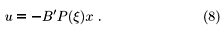
IICenter for Control Engineering and Computation, University of California, Santa Barbara, CA, 93106, USA

IIIDepartamento de Automação e Sistemas, Universidade Federal de Santa Catarina Florianópolis, SC, 88040-900, Brazil

^{Adress to correspondence}

ABSTRACT

This paper deals with the global stabilization problem of linear systems with saturating actuators. Global stabilization is achieved by scheduling a parameterized control law constructed from a parameterized solution of the algebraic Riccati Equation (ARE). The scheduling algorithm is guided by the magnitude of the control signal and reduces conservativeness of similar existing schemes. Several important properties of this algorithm regarding its functionality, design parameters, implementation issues, and capabilities are discussed. Simulation results for a case study are included illustrating the main features of the control scheme and the overall performance of the closed loop system.

Keywords: Saturation, global stabilization, scheduling, Riccati equation.

RESUMO

Este trabalho trata do problema da estabilização global de sistemas lineares com saturação nos atuadores. A estabilização global é obtida por meio de uma estratégia de escalonamento de ganho, aplicada a uma lei de controle parametrizada construída a partir de uma família de soluções da equação de Riccati (ARE). O algoritmo de escalonamento é guiado pela magnitude do sinal de controle e reduz a conservatividade de algoritmos similares existentes. Diversas propriedades deste algoritmo são discutidas relativamente a sua funcionalidade, parâmetros de projeto, aspectos de implementação e potencialidades. São incluídos resultados de simulação para um estudo de caso ilustrando as principais propriedades do algoritmo e o desempenho geral do sistema em malha fechada.

Palavras-chave: Saturação, estabilização global, escalonamento de ganho, equação de Riccati.

1 INTRODUCTION

Stabilizing linear systems with saturating actuators has been a fast growing research topic in the last decade. While local stabilization is always possible, achieving global stabilization and/or enlarging the region of attraction are more delicate issues. Necessary and sufficient conditions for global stabilizability of linear systems with bounded controls have been given in (Sontag and Sussman, 1990). The requirement is that the pair (A,B) be stabilizable and all the eigenvalues of A have non-positive real part, a requirement that is equivalent to the linear system being asymptotically null-controllable with bounded controls (Schmitendorf and Barmish, 1980).

In general, the global stabilization of linear systems with saturation requires nonlinear feedback (Sontag and Sussman, 1990; Teel, 1992; Sussman et al., 1994; Teel, 1996; Megretski, 1996). As a matter of fact, even a chain of 3 or more integrators cannot be globally stabilized by linear feedback (Fuller, 1969). Nonetheless, semi-global stabilization by linear feedback was proven in (Lin and Saberi, 1993; Teel, 1995b; Saberi et al., 1996) by synthesizing linear feedback control laws based on a parameterized family of solutions of both the Riccati equation and the H_¥-type Riccati equation. Semi-global stabilization with performance improvements is also considered in (Wredenhagen and Belanger, 1994; Saberi et al., 1996).

Generating control laws on the basis of parameterized ARE (algebraic Riccati equation) solutions led to important achievements in the control of this class of systems. The main property of this construction is the possibility of synthesizing a nested family of ellipsoidal sets which can be rendered positively invariant for the closed-loop system by appropriately choosing the value of the parameter in the parameterized control law. Such property has been exploited to achieve global stabilization by implementing an on-line scheduling of the parameterized control law according to the evolution of the state (Teel, 1995a; Megretski, 1996; Lin, 1998). The general intuition is to use low gain when the state is large (to ensure stability) and to allow the gain to be higher when the state is small (to speed up convergence). The scheduling of the parameterized control law is also a degree of freedon that can be used to improve performance of the closed-loop system over to well know low gain designs for semiglobal stabilization.

The estimates based on ellipsoidal sets, however, are in general conservative, a fact that limits closed-loop system performance since the assigned gain is usually smaller than it could be. An attempt to reduce such conservativeness was made in (Reginatto et al., 2000b; Reginatto et al., 2000c), where a scheduling mechanism guided directly by the magnitude of the control signal was proposed. The scheme does not employ estimates based on ellipsoidal sets and allows the scheduling parameter to be non-monotone in time as opposed to the schemes in (Megretski, 1996; Lin, 1998).

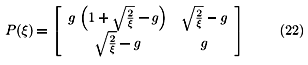
In this paper we focus on the scheme of (Reginatto et al., 2000b; Reginatto et al., 2000c) to schedule a parameterized control law constructed from a parameterized ARE solution. The scheme is given a thorough analysis revealing its functionality, degrees of freedom, design parameters, and performance achievements. An illustrative case study is worked out showing the main features of the scheduling algorithm.

The paper is organized as follows. The main theory is presented in Section 2 where the scheduling algorithm is presented. Section 3 analyzes the functionality of the scheduling algorithm, the design parameters, and implementation issues. In section 4, simulation results are presented for a case study illustrating the behavior of the algorithm. Finally, the paper is concluded in section 5. Proofs are included in the appendix.

2 THE SCHEDULING ALGORITHM

We consider linear systems with input saturation given in the form

where x Î Rⁿ is the state, u Î R^m is the control input, and s(·) is a locally Lipschitz decentralized saturation function which is globally bounded and satisfies

where sat_D(u) is the standard decentralized saturation function of magnitude D, i.e.,

where sat_D(u_i) = sign(u_i)max{|u_i|,D}. Also assume that the pair (A, B) is stabilizable.

To consider the global stabilization problem, we introduce the following necessary assumption (Sontag and Sussman, 1990),

Assumption 1 No eigenvalue of A has strictly positive real part¹.

In the next lemma (see (Teel, 1995a)) we introduce the main ingredients of the construction of the parameterized control law which will be employed in our scheduling algorithm. This control law is constructed on the basis of a parameterized family of solutions of a parameterized Algebraic Riccati Equation. For a proof of this lemma see (Teel, 1995a).

Lemma 1Let Q:[1,¥)®R^n×n be a continuously differentiable matrix valued function such that lim_x®¥Q(x) = 0 and, for all x Î [1, ¥),

Then, for system (1), there exists a continuously differentiable matrix valued function P(x) satisfying for all x Î [1, ¥),

Moreover, if Assumption 1 holds, then P_o = 0.

Using the matrix valued function P(x) generated according to Lemma 1, we generate the parameterized control law

As x ranges from 1 to ¥, P(x) approaches the constant P_o matrix. In this way, the magnitude of the control "gain'' can be varied by varying the parameter x. Since P(x) is monotone, x = 1 yields the largest control "gain'' and will be referred to as the nominal value for x. In the case P_o = 0, the controller "gain'' can be made as small as desired by choosing large values of x. The ability to change the control gain by varying x is the main property used by scheduling algorithms to achieve global stabilization.

Most scheduling algorithms (Teel, 1995a; Megretski, 1996; Lin, 1998) determine x by looking at the level sets of a x-dependent quadratic positive definite function of the state, for instance,

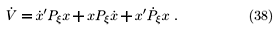
As a result of the scheme, the state trajectory is confined to ellipsoidal positive invariant sets and the scheduling parameter x results monotone in time. These are the properties that we want to focus on, as they inherently introduce some degree of conservativeness in the scheme, leading to controller "gains'' that are smaller than stability itself would require. So, we are interested in avoiding such properties in the control scheme, while still guaranteeing global asymptotic stability. An attempt in such direction is made in the scheduling algorithm presented next (Reginatto et al., 2000b; Reginatto et al., 2000a).

The following definition states the main ingredients for the scheduling algorithm.

Definition 1 Consider system (1) and the notation of Lemma 1.

1. Let a Î (0, 1), r Î (0, 2D], and b Î [0, min{1, (2D-r)/r}] be real constants. Define,

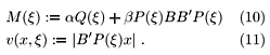
2. Let L:Rⁿ×R_{³ 0}®[0,1] be a globally Lipschitz function satisfying

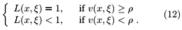
3. For k Î (0,2D) let r:R×Rⁿ®R_{³ 0} be a locally Lipschitz function satisfying for all (x, x) Î [1, ¥)×{Rⁿ\{0}},

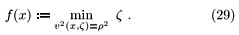
4. Let G(x): = { x Î [1,¥): v(x,x) £ r}.

The scheduling algorithm (Reginatto et al., 2000b; Reginatto et al., 2000c) consists in an operator (x(0), x(t), L(x(t)), x(t)), with x(0) Î G(x(0)), that yields x(t) according to

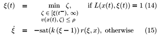
where k is a positive constant (design parameter) and x(t^-): = lim_{t® t^-}x(t).

With the scheduling algorithm (14)-(15) for the control law (8), asymptotic stability is achieved for the closed-loop system, as stated in the next theorem.

Theorem 2Let P(x) and Q(x) be as in Lemma 1. Consider the notation introduced in Definition 1. Then, system (1) with the control law (8) and the scheduling algorithm (14)-(15) is such that x = 0 is locally exponentially stable. If, in addition, the Assumption 1 holds, then x = 0 is globally asymptotically stable. Moreover, in any case, x(t)® 1 as t® ¥.

Proof. See appendix.

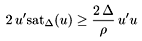
The scheduling algorithm (14)-(15) is guided by the signal v(x(t), x(t)), which corresponds to a measure of the magnitude of the control signal u. The actual constraint imposed by the scheduling algorithm is that

By comparing (16) and (9) one can grasp the amount of conservativeness reduction achieved by our scheduling algorithm. Although we have used the Euclidean norm to define v(x,x) as a measure of the magnitude of the control signal, it is actually possible to employ any p-norm for p Î [1,¥). This may be of interest for multi-input systems since, in this case, v(x,x) will give different estimates for different p-norms.

3 PROPERTIES OF THE SCHEDULING ALGORITHM

The scheduling algorithm has the nature of a hybrid system as the dynamics of x(t) are given either by (14) or (15). The transitions from one to another dynamics for x(t) are dictated by the function L which depends on the state x and the scheduling parameter x. The funcion L is actually an indicator for the magnitude of the control signal, as measured by the function v(x,x). Since the control signal depends on x, the scheduling mechanism (14)-(15) is actually defined as an implicit relation in x(t). The following reasoning will clarify this issue, while addressing the functionality of the scheduling algorithm, and show that the scheme is in fact well defined.

Recovery phase. When the control signal is small (L < 1), the scheduling parameter x(t) is given by (15). Since r is non-negative, x(t) is non-increasing in time. In particular, in the region where r(x,x) > 0, x(t) is strictly decreasing. The saturation function in (15) plays its role when x(t) is close to one, in which case it guarantees x = 1 to be an equilibrium point. Thus, when the control signal is small, the scheduling parameter is non-increasing and converging to 1, its nominal value. This phase of the scheduling parameter constitutes the recovery phase, in which the "gain'' of the controller is pushed towards its maximum value.

Attaining phase. On the other hand, when the magnitude of the control signal grows large (L = 1), the scheduling parameter x(t) is given by (14). The aim in this phase is to reduce the controller "gain'' as much as necessary to prevent the control signal to exceed the amount of saturation as given by the parameter r. This is achieved by solving the minimization problem in (14). It guarantees v(x(t),x(t)) £ r for all t, thus yielding the desired property. In fact, the equality v(x(t),x(t)) = r holds during the time (14) is active. This is possible as long as the required gain is larger than the limit value determined by P_o, thus characterizing the nature of the local stability property in Theorem 2. In case the Assumption 1 holds, for any x we can find a x, large enough, such that v(x,x) = r, since lim_x®¥P(x) = 0.

Discontinuity. In the minimization problem (14) x is constrained to be non-decreasing, which is a fundamental property to ensure stability of the closed-loop system. Since v(x,x) is not necessarily monotone in x, constraining x(t) to be non-decreasing may lead to discontinuities in the scheduling parameter. However, such discontinuity in x(t) does not cause a discontinuity in v(x(t),x(t)) by the definition of the minimization problem. Thus, the actual control signal u is not necessarily discontinuous at such points. For instance, in the single-input case, the regularity of the parameterization and the continuity of v(x(t),x(t)) in time implies continuity of u(t).

Transitions. Let us now consider the transition from (14) to (15) and vice-versa. Assume, for instance, that the system initialization satisfies L(x(0),x(0)) < 1. As the system evolves in time, the condition L(x(t), x(t)) = 1 may be attained. If that is the case, the definition of the function r(x,x) ensures that x(t) is constant as the condition L(x(t), x(t)) = 1 is approached. Thus, only the state is able to cause a transition from (15) to (14). On the other hand, if the closed-loop system is operating with L(x(t), x(t)) = 1, the minimization problem ensures v(x(t),x(t)) = r. Thus, similarly, only the state is able to cause a transition from (14) to (15). As a result, the transition is smooth since it is guided only by the state. Moreover, since L is continuous as a function of time, the scheduling algorithm can always be started by checking the value of L and then computing x(t). This solves the implicit problem in the statement of the scheduling algorithm.

Remark 1 As far as the discontinuity issue is concerned, it is important to remark that there is no possibility for fast switching in the parameter x. As a matter of fact, discontinuities can only happen when v(x(t),x(t)) = r, in which case x(t) is given by (14). By the smoothness of the function v and the nature of the minimization problem, one can show that discontinuity points are isolated and only a finite number of them can exist in any bounded time interval. A more comprehensive treatment of this issue is given in the proof (see appendix).

Parameters: The most important parameter in the scheduling algorithm is the function r(x,x). It determines the rate of recovery of the scheduling parameter x(t). In general, the faster the recovery, the higher the controller "gain'' and thus the better the performance. Thus, we are in general interested in choosing r as large as possible. A simple and natural choice is

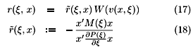
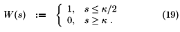
where W(·) is a locally Lipschitz function satisfying

An alternative choice for r(x, x) is as follows. Let :R®R _{> 0} be a locally Lipschitz and globally bounded function satisfying

Then, we just replace (x,x) in (18) by the one in (20). The function (·) in (20) can be given a closed form and it is computationally less expensive than (18). The price paid is that the recovery of x may become considerably slower.

The parameter a affects the function r through M(x). A larger a allows for a larger r and, consequently, a faster recovery rate for x. However, the actual effect on the closed-loop system performance depends on the parameterized ARE solution at hand, namely, whether Q(x) dominates or not the right hand side of M(x). Moreover, the convergence rate that can be proved for the state depends on (1-a) a fact that may lead to a trade-off in the choice of a. The parameter b plays as similar role as a with respect to the term P(x)BB¢P(x).

The role of the parameter k is to ensure a smooth transition between the increasing (14) and recovery (15) phases of the scheduling algorithm. Its effect on the actual recovery rate can be minimized by choosing k close to r.

Remark 2 The admissible level of saturation is set by the parameter r. If of interest, saturation of the control signal can be avoided by choosing r £ D. On the other hand, by exploiting the gain margin of the control law (8) we can allow r up to 2D, thus possibly improving the closed-loop system performance. However, in the presence of uncertainties in the control input, it may be wise to set r not close to its limiting value.

Implementation issues: The minimization problem (14) required in the scheduling mechanism consists in a nonlinear programming problem. However, since the decision variable is scalar (one-dimensional), the problem is easily tractable with standard algorithms. For instance, a simple search combined with the bisection algorithm can be successfully applied.

Since actual implementation of control algorithms are in general in discrete-time, it is important to consider the effect of the discretization of the scheduling algorithm. In fact, a discrete-time implementation is highly desirable since the continuous solving of the minimization problem is not practical. A natural approach is to employ fast sampling and a discrete-time approximation for (15). In this case, however, the result will be only semi-global, i.e., stability of the origin can only be guaranteed for initial conditions in a certain compact set in the state space. The smaller the sampling time, the larger the stability domain, this being the meaning of semi-global. Nonetheless, the result is still satisfactory for most practical applications.

4 SIMULATION RESULTS

The following example is taken from (Lin, 1998) and consists in a chain of 2 integrators with state-space representation given by

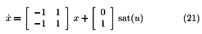
where the control signal is constrained by a standard saturation function of magnitude one. The parameterized solution of the ARE (Lemma 1) is constructed for Q(x) = (1/x) I. It is given in closed form by (Lin, 1998)

where g : = .

The function r(x,x) is chosen according to (17) with

for a = 0.9, r as indicated in each case, and k = 0.95r. In all simulations k = 10, x is initialized at 1, whenever possible, and the scheduling algorithm is implemented in discrete time with a sampling period of 5ms.

The behavior of the closed-loop system is illustrated in Figure 1. For the small initial condition the system saturates only at the beginning and the scheduling parameter is monotone in time. For the large initial condition, the scheduling parameter exhibits its non-monotone property since the control signal reaches its limits twice in this case. In both cases, the state converges to the origin and the scheduling parameter recovers its nominal value with a similar rate as the state goes to zero.

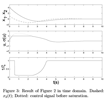
The functionality of the scheduling algorithm can be visualized in the 3D plot shown in Figure 2, thanks to the system being of second order. The scheduling algorithm enforces the closed-loop system to operate in the region S: = { (x,x): v(x,x) £ r}, which corresponds to the space between the surfaces in the figure. The scheduling parameter starts at x = 1 and is constant up to the time the trajectory reaches the boundary of S (the ° point in the picture). At that point, a discontinuity in the scheduling parameter takes place because the right boundary of S has a concave shape close to x = 1 (viewed from the right) so that, if x were increased slightly from 1, a shrink of S would be obtained instead of an enlargement. Then, x jumps to a point where the region S enlarges as x increases (D) and continues increasing keeping the trajectory on the boundary of S. After the Ÿ point, the trajectory leaves the boundary of S and converges to the origin (of the (x₁,x₂) space) while the scheduling parameter is slowly decreased to its nominal value. One can observe that x is constant both when the trajectory reaches the boundary of S and when leaving it. The same result is shown in time domain in Figure 3.

The effect of the parameter r on the closed-loop system performance can be seen in Figure 4. We see that the maximum value of r = 2 allows a faster convergence of the state than for the case r = 1. The scheduling parameter illustrates that a higher control gain is employed in the case r = 2 allowing the control signal to saturate as opposed to the case r = 1. One can also observe the monotonicity of the scheduling parameter in this case.

In Figure 5 we investigate the influence of the function r(x,x) in the performance of the closed-loop system and the scheduling parameter x(t). As previously mentioned, it might be of interest to reduce computation effort by choosing a closed form expression for as a function only of x. We make the following simple choice

The required properties for r(x,x) are, with some conservativeness, satisfied with this choice and W(v(x,x)) given by (24). The result in Figure 5 shows that the recovery of the scheduling parameter gets considerably slower causing the convergence of the state to be more sluggish. Thus, the choice for r becomes a trade-off between performance and implementation complexity.

For completeness (see also (Reginatto et al., 2000b)), we also include Figure 6 which compares the performance of the scheduling algorithm with the scheme in (Megretski, 1996). The scheduling mechanism based on the control signal achieves a faster convergence of the state and more effective use of the available control effort. The result confirms the inherent conservativeness of the scheme based on ellipsoidal sets (Megretski, 1996; Lin, 1998), and that the rationale behind the presented scheduling algorithm indeed leads to a less conservative result.

5 CONCLUSION

We have investigated a scheduling mechanism for a parameterized ARE solution aimed at achieving global asymptotic stability for linear systems with saturating actuators with improved performance.

The fact that the scheduling mechanism is guided directly by the magnitude of the control signal (instead of ellipsoidal sets) allows for both reduced conservativeness and non-monotone (in time) scheduling parameter. Although the scheduling parameter is not guaranteed to be continuous in time, a fact that may introduce discontinuities in the control signal, the closed-loop system is well behaved in the sense that the trajectories are piecewise C¹ in time.

The scheduling algorithm can be implemented in discrete-time employing fast sampling. The stability property is semi-global in this case, the domain of stability enlarging as the sampling period is reduced. Complexity of implementation may be reduced by choosing a closed form expression for r as a function of x only, although possibly at the expense of closed-loop system performance.

Simulation results have been presented illustrating the main properties of the scheduling algorithm.

A PROOF OF THE MAIN RESULT

Throughout the proof we drop the t dependence of most variables for simplicity. Also, we write P_x for P(x), and similarly for other matrix valued functions.

Existence of solutions Since the minimization problem (14) constraints x(t) to be non-decreasing in time, a more careful analysis is required regarding the existence of solutions for the closed-loop system.

Given any x_oÎ Rⁿ and x_oÎ G(x_o), we mean by a solution for system (1), (8), (14), (15) a continuous and piecewise C¹ function of time x(t) defined on some time interval [t_o,t₁) which satisfies, together with a (possibly discontinuous) piecewise C¹ function x(t), x(t_o) = x_o, x(t_o) = x_o, and (1), (8), (14), (15) for almost all t Î [t_o,t₁).

We claim that solutions for the closed-loop system exist for all initial states x(t_o) Î Rⁿ consistent with the set

Moreover, in case Assumption 1 holds, solutions exist for all initial states in Rⁿ and are defined for all forward time. To see this, consider the two systems

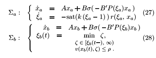
We shall construct solution for the closed-loop system by patching solutions of systems S_a and S_b. Let's first consider these two systems separately.

Clearly S_a has a unique solution for each (x(t_o), x(t_o)) Î Rⁿ ×[1,¥) which is defined for all forward time and is a continuously differentiable function of time.

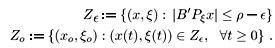
For the analysis of system S_b, first notice that the minimization problem yields a non-decreasing function of time x _b(t) which is constant whenever v(x _b(t), x_b(t)) < r. Thus, x _b(t) is continuous ² for almost all t ³ 0 in the time interval for which a solution for system S_b is defined. Moreover, discontinuities can only take place at time instants where the constraint is effective, i.e., in the set : = { t: v(x_b(t), x _b(t)) = r}.

Consider the auxiliary problem

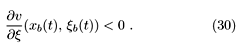
Since v(x,z) is C¹, f(x) will be C¹ in a neighborhood of any point such that (x,f(x)) ¹ 0. From this fact, it follows that for any x_b(t_o) Î Rⁿ and x_b(t_o) Î G(x _b(t_o)) such that (¶v/¶x)(x_b(t_o),x_b(t_o)) < 0, the system S_b has a unique solution defined for some interval [t_o, t₁) with the property that, for all t Î [t_o, t₁), x _b(t) is continuous and

Clearly, the solution can be continued over time as long as (30) is satisfied. Since x _b(t) is constrained to be non-increasing, the violation of condition (30) may lead to a discontinuity. If a discontinuity takes place at t = t₁, necessarily ³

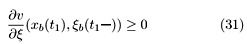
and x _b(t₁) obtained from S_b will satisfy (30) at t = t₁. Thus, a unique solution for system S_b will exist over an interval [t₁, t₂) starting from x_b(t₁) and x_b(t₁). Clearly, for any x_b Î Rⁿ such that |B¢P_ox_b| < r there exist a x _b satisfying (30). Moreover, the continuous differentiability of P(x) guarantees that only a finite number of discontinuities may occur in any compact time interval, thus allowing to extend solutions of system S_b by repeating the same argument for as long as the minimization problem has a finite solution. This is always the case if Assumption 1 holds.

Let's now patch the trajectories of S_a and S_b to construct solutions for the closed-loop system. Let (x(t_o), x(t_o)) Î Rⁿ×[1,¥) and assume, without loss of generality, that v(x(t_o), x(t_o)) < r. Let (x_a(t_o), x_a(t_o)) = (x(t_o), x(t_o)). Thus, (x(t), x(t)) = (x_a(t), x_a(t)) as long as v(x_a(t), x_a(t)) < r. Let t₁ > t_o be the first time v(x_a(t), x _a(t)) = r. Assume t₁ < ¥, otherwise we would be done. Set x_b(t₁) = x_a(t₁) and x_b(t₁-) = x_a(t₁) = x(t₁-). Now, (x(t), x(t)) = (x_b(t), x _b(t)) as long as v(x_b(t), x _b(t)) = r. Let t₂³ t₁ be the last time this condition is satisfied for system S_b. Thus, $ d₁ > 0 such that v(x_b(t), x _b(t)) < r and _b(t) = 0 for all tÎ (t₂,t₂+d₁). Set (x_a(t₂), x_a(t₂)) = (x_b(t₂), x _b(t₂)). Since W(·) is (Lipschitz) continuous and W(v(x,x)) = 0 whenever v(x,x) ³ k, it follows that for some d₂ > 0, d₂£ d₁, (x_a(t), x_a(t)) = (x_b(t), x_b(t)) in (t₂, t₂+d₂) and thus v(x_a(t), x_a(t)) < r in (t₂, t₂+d₂). Thus (x(t), x(t)) = (x_a(t), x_a(t)) for all t > t₂ such that v(x_a(t), x_a(t)) < r. Such property holds at least for an open time interval so that high frequency switching (sliding-mode) between (14) and (15) is not possible.

By repeating the same reasoning, solutions of the closed-loop system can be continued over time for as long as the minimization problem (14) has a finite solution. It follows that x(t) is continuous and piecewise C¹, while the scheduling parameter x(t) is piecewise C¹ and, possibly, discontinuous at isolated time instants, which add up to, at most, a finite number in any compact time interval.

Local Exponential Stability Let e > 0 and define the sets

Clearly, Z_o is well defined (not necessarily compact) and has a non-empty interior. For initial conditions in the set Z_o, x(t) is given by (15) for all times. Then, for the continuously differentiable positive definite function

we obtain

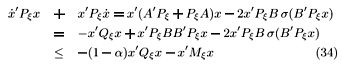
Using (5), (10), (13) and Lemma 3, we obtain,

and

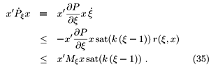
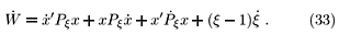
Collecting (34) and (35) into (33) and computing from (15) yields

It follows from (32) and (36) that the point (x,x) = (0,1) is locally exponentially stable.

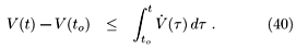
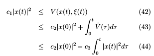
Global Asymptotical Stability Solutions of the closed loop systems, whenever defined, belong to the set Z (see eq. (26)). Consider the positive definite function

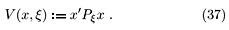
Since x(t) and x(t) are piecewise continuously differentiable so is V(x(t),x(t)). Thus, for almost all t ³ 0, we evaluate the time derivative of V(x,x) along trajectories contained in Z to obtain

We again obtain (34) and (35), which now hold for almost all t ³ 0, leading to

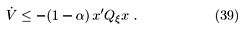
Clearly, is piecewise continuous and can be integrated on any compact time interval. Moreover, V(x(t),x(t)) decreases at any discontinuity point of x(·) because x(·) is continuous, ¶P_x/¶x < 0, and x(·) increases at any such point. From this fact, and since only a finite number of discontinuity points of V(x(t),x(t)) can exist in any compact time interval, we can state that (see also (Jones, 1993, Chap 16))

Then, (40) and (39) yield

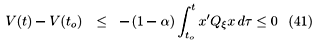
implying that V(t) is bounded. So, in particular, x is bounded. In turn, this implies that x(t) is bounded, i.e., $ such that x(t) Î [1, ], "t ³ t_o. For, otherwise v(t) = |P^1/2(x(t) [P^1/2(x(t))x(t)]|® 0 as t®¥ and there would exist a T ³ t_o such that v(t) £ r/2, "t ³ T. Thus, x(t) would be decreasing for all t ³ T, which contradicts the fact that x(t) is unbounded.

Boundedness of x implies that both |P(x)| and |Q(x)| are bounded away from zero, implying that there exist constants c₁ > 0, c₂ > 0, and c₃ > 0 (depending on ) such that for all t ³ 0 (using (41))

which proves the result.

A.1 Technical lemma

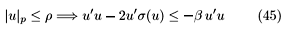
Lemma 3Let 0 < r £ 2D and b:= min{1, (2D-r)/r}. Let s(·) be locally Lipschitz and such that u¢s(u) ³ u¢sat_D(u), "u ÎR^m. Then, for any p Î [1, ¥],

where |·|_p is the usual p vector norm.

Proof: First notice that the right hand side of (45) is implied by

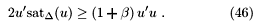
It is clear that (46) holds for 0 < r £ D since, in this case, b = 1 and sat_D(u) = u. For the case D < r £ 2D, notice that |u|_p£ r implies |u_i|_p£ r for i = 1,¼,n. In turn, |u_i|_p = |u_i| £ r implies

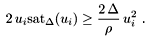
Consequently,

from which the result of the lemma follows.

ž

ACKNOWLEDGMENT

R. Reginatto is supported in part by CAPES. A. R. Teel is supported in part by NSF under grant number ECS-9896140.

Andrew R. Teel

E-mail: [e-mail]

Edson R. De Pieri

E-mail: [e-mail]

Artigo submetido em 20/12/00

1a. Revisão em 04/04/02

Aceito sob recomendação do Ed. Assoc. Prof. Liu Hsu

• Fuller, A. T. 1969 . In-the-large stability of relay and saturating control systems with linear controller, Int. Jornal of Control 10: 457-480.
• Jones, F. 1993 . Lebesgue Integration on Euclidean Space, Jones and Bartlett Publishers, USA.
• Lin, Z. 1998 . Global control of linear systems with saturating actuators, Automatica 34(7): 897-905.
• Lin, Z.  Saberi, A. 1993 . Semi-global exponential stabilization of linear sytems subject to input saturation via linear feedbacks, Syst. Cont. Letters 21(3): 225-239.
• Megretski, A. 1996 . ₂ BIBO output feedback stabilization with saturated control, Triennial IFAC World Congress, San Francisco, USA, pp. 435-440.
• Reginatto, R., Teel, A. R.  de Pieri, E. R. 2000a . Enhanced performance global stabilization of linear systems with saturating actuators, XIII Congresso Brasileiro de Automática, Florianópolis, Brasil, pp. 949-954.
• Reginatto, R., Teel, A. R.  de Pieri, E. R. 2000b . Performance enhancement and robustness for linear systems with saturating actuators, 3rd IFAC Symposium on Robust Control Design, ROCOND'2000, Prague, Czeck Republic.
• Reginatto, R., Teel, A. R.  de Pieri, E. R. 2000c . Stabilization of saturated linear systems: A scheduling mechanism based on the control signal, Relatório técnico, Universidade Federal de Santa Catarina, Florianópolis, Brazil.
• Saberi, A., Lin, Z.  Teel, A. R. 1996 . Control of linear systems with saturating actuators, IEEE Trans. Aut. Cont. 41(3): 368-378.
• Schmitendorf, W. E.  Barmish, B. R. 1980 . Null controllability of linear systems with constrained controls, SIAM J. Cont. Opt. 18(4): 327-345.
• Sontag, E. D.  Sussmann, H. J. 1990 . Nonlinear output feedback design for linear systems with saturating actuators, Conference on Decision and Control, Honolulu, Hawaii, pp. 3414-3416.
• Sussmann, H. J., Sontag, E. D.  Yang, Y. 1994 . A general result on the stabilization of linear systems using bounded controls, IEEE Trans. Aut. Cont. 39(12): 2411-2424.
• Teel, A. R. 1992 . Global stabilization and restricted tracking for multiple integrators with bounded controls, Syst. Cont. Letters 18: 165-171.
• Teel, A. R. 1995a . Linear systems with input nonlinearities: Global stabilization by scheduling a family of _Ľ-type controllers, Int. J. Robust Nonlinear Control5: 399-411.
• Teel, A. R. 1995b . Semi-global stabilizability for linear null controllable systems with input nonlinearities, IEEE Trans. Aut. Cont. 40(1): 96-100.
• Teel, A. R. 1996 . A nonlinear small gain theorem for the analysis of control systems with saturation, IEEE Trans. Aut. Cont. 41(9): 1256-1270.
• Wredenhagen, G. F.  Belanger, P. R. 1994 . Piecewise-linear LQ control for systems with input constraints, Automatica 30(3): 403-416.

1

Notice that the plant may be open-loop unstable, although it cannot contain any exponentially unstable mode (eigenvalue with strictly positive real part).

2

A non-negative and monotone function is continuous at almost every point in its domain (Jones, 1993, Chap. 16).

3

Notice that

x_b(·) is continuous at

t

₁.

Publication Dates

• Publication in this collection
  10 Apr 2003
• Date of issue
  Mar 2003

History

• Reviewed
  04 Apr 2002