Prediction of Stamp Impression Age Based on Hyperspectral Imaging Technology and Machine Learning

Abstract

The accurate determination of stamping time holds significant importance for forensic document examination and authentication. To address the critical challenge of determining the age of stamp impressions in document forensics, this study proposed a non-destructive predictive method based on hyperspectral imaging (HSI) technology and support vector machine (SVM) algorithm for estimating the stamping age. Hyperspectral data were collected from stamp impressions made with two oil-based inks at 27 time points, spanning a range of 0.42 to 205 days. A predictive model for impression age was constructed by integrating these data with SVM algorithm. This model was systematically compared against other machine learning (ML) approaches. The experimental results demonstrated that the SVM model achieved optimal performance on the test set, with a Nash-Sutcliffe efficiency coefficient (NSE) of 0.99 and a root mean square error (RMSE) of 7.69 days. This performance significantly surpassed that of the extreme learning machine (ELM) model (NSE = 0.78, RMSE = 24.64 days), the backpropagation neural (BP) network (NSE = 0.95, RMSE = 12.19 days), the partial least-squares (PLS) model (NSE = 0.84, RMSE = 20.68 days), and the long short-term memory (LSTM) model (NSE = 0.94, RMSE = 12.89 days). This study provided a novel technical reference for the accurate prediction of stamp impression age.

Keywords:
hyperspectral imaging; support vector machine; oil-based stamp ink; age prediction

Introduction

A seal serves as an identifying mark, typically administered and utilized by authorized institutions or organizations, to authenticate and legitimize documents through the application of red ink impressions. In Asian countries, seal application represents a widely prevalent practice, extensively employed in documents involving substantial economic value,¹ such as real estate transactions, financial operations, bank accounts, insurance claims, and wills. The validity of a document typically requires that the stamping time aligns precisely with the creation time of the document text. Any temporal inconsistency may cast doubt on the authenticity of the documents, potentially leading to serious legal disputes and economic losses.² Recent judicial practices indicate that crimes related to forged seals are becoming increasingly complex, with the incidence rising year by year. According to recent reports, the vietnamese court system handled 652 cases related to forged seals and stamping time in 2024 alone, representing a 3.45-fold increase compared to 2020.³ In this context, the precise and non-destructive determination of the age of stamped impressions has emerged as a critical and challenging task in forensic science and questioned document examination.

Traditional methods for determining the age of seal imprints primarily rely on physic-chemical analysis techniques.⁴-⁶ These methods involve highly complex and time-consuming processing procedures. Upon transfer to paper, stamp ink undergoes aging through dye demethylation (light-induced), solvent evaporation, and resin polymerization. Liquid chromatography employs chromatographic and spectroscopic techniques to analyze changes in the dye structure of ink such as demethylation, solvent evaporation, and resin polymerization to determine the age of stamp ink.⁷,⁸ Researchers applied this method to five cases referred to the court at the time, demonstrating inconsistencies between the stamping time and the creation time of the contract text.⁶ However, these methods are not only extremely complex and time-consuming, but also require expensive instrumentation with high operational and maintenance costs, as well as specially trained personnel for operation. Researchers conducted statistical analysis by calculating and capturing relevant color features from scanned images. They used K-means for clustering and subsequently integrating the analytical outcomes for decision-making, achieving an overall accuracy of 74.5%.⁹ While this method avoids damage to the document, it relies on numerous assumptions, rendering it impractical for real-world applications. Researchers proposed a document age determination model based on the background color components of scanned images.¹⁰ The model employs a digital microscope to analyze the red, green and blue (RGB) histogram of document paper and infers the age of the document based on variations in RGB components. Nevertheless, this approach is constrained by stringent requirements: the paper must be free of any stains or handwriting, and it is generally only effective for documents spanning extended periods (43 to 50 years). To some extent, the physical-chemical analysis methods described above for determining document age can reflect changes in seal ink composition over time. However, these approaches are destructive, often causing irreversible damage to original documents. Moreover, they involve complex procedures and exhibit poor reproducibility, making it difficult to meet the requirements of modern forensic science for non-destructive, efficient, and objective analysis.¹¹ Furthermore, the aging process of stamp ink is significantly influenced by environmental factors such as temperature, humidity, and light exposure as well as variations in ink composition, which limits the accuracy of traditional methods over extended time frames. Spectroscopic techniques, such as Fourier transform infrared spectroscopy¹² and Raman spectroscopy,² have been introduced to provide more detailed information on the chemical composition of stamp inks, while also overcoming the destructive limitations of conventional physicochemical methods. However, as point-based measurement techniques, they can only analyze localized areas of the stamp impression, which may not adequately represent its spatial and temporal heterogeneity, and their analytical performance is susceptible to interference from the substrate background. Therefore, developing a nondestructive, rapid, and reliable method for determining the age of stamp impressions is of significant theoretical value and practical importance.

In recent years, hyperspectral imaging (HSI) technology has emerged as a powerful non-destructive analytical tool, demonstrating broad application prospects across fields such as food engineering,¹³ agricultural product quality analysis,¹⁴ cultural heritage preservation,¹⁵ forensic science,¹⁶ and non-destructive document examination.¹⁷,¹⁸ In contrast to conventional spectral techniques, HSI can simultaneously acquire both spatial information and full spectral data (ranging from visible to near-infrared wavelengths) of a sample, generating a three-dimensional hypercube dataset comprising hundreds of continuous bands. This enables the detection of subtle chemical changes that are imperceptible to the human eye. This capability makes HSI particularly suitable for detecting subtle and spatially heterogeneous chemical changes induced by ink aging processes such as solvent volatilization, dye oxidation, and resin polymerization.¹⁹ These changes manifest as systematic variations in spectral reflectance at specific wavelengths. However, existing research on document verification using HSI primarily focused on distinguishing ink types and identifying their sources.¹⁹ Systematic studies applying HSI to quantitatively predict the formation time of seal impressions remain scarce. Seal ink undergoes a series of physicochemical reactions over time after application, including volatilization, oxidation, and cross-linking. These processes cause systematic changes in its spectral characteristics, providing the theoretical basis for applying hyperspectral imaging technology to the chronological authentication of seal impressions.

Simultaneously, machine learning methods have demonstrated strong capabilities in pattern recognition and regression prediction for spectral data analysis. They can extract key features from high-dimensional data and establish robust predictive models,²⁰ offering a new technical pathway for the chronological authentication of seal impressions. Support vector machine (SVM) is an algorithm particularly suitable for handling highdimensional, small-sample datasets. By employing kernel functions to map data into high-dimensional space, it identifies an optimal regression hyperplane. This method has been successfully applied, for examples, in the rapid identification of bloodstain types using near-infrared spectroscopy, processing of remote sensing (RS) data and determination of flavor value of rice.²¹-²³ As a classic nonlinear model, the backpropagation neural network (BP) is theoretically capable of approximating any complex function. However, its training process is slow, requires extensive parameter tuning, and is prone to becoming trapped in local minimum.²⁴ Extreme learning machine (ELM), a variant of single-hidden layer feedforward neural networks, has gained attention for its extremely fast training speed. Nevertheless, its random initialization of weights and biases may lead to poor stability in prediction results.²⁵ Partial least squares regression (PLS), a linear method commonly used in chemometrics, can effectively handle high-dimensional collinear data but has limited capacity for modeling nonlinear relationships.²⁶ Long short-term memory (LSTM) is a specialized form of recurrent neural network, offering advantages in processing sequential data.²⁷,²⁸ However, its performance on non-sequential high-dimensional features such as spectral data remains unexplored. Currently, there is a lack of research systematically evaluating and comparing the performance of these machine learning algorithms in predicting the age of seal impressions based on hyperspectral data.

Based on the aforementioned analysis, this study proposes a non-destructive method for predicting the age of stamped impressions by integrating hyperspectral imaging with SVM, termed HSI-SVM. The primary objectives of this research are threefold: (i) to systematically acquire hyperspectral data from oil-based stamp inks of different brands across multiple time points; (ii) to develop an SVM-based regression model, optimized through preprocessing techniques such as multiplicative scatter correction (MSC), for accurate stamp age prediction; and (iii) to comprehensively evaluate the proposed method against four benchmark machine learning algorithms PLS, ELM, BP, and LSTM to validate its superiority and reliability.

The main contributions of this work include: (i) we demonstrate, for the first time, the feasibility of combining HSI with SVM for non-destructive stamp age determination; (ii) we provide a systematic comparison of various machine learning approaches for this forensic application; (iii) we establish an efficient and objective technical framework that advances document examination toward non-destructive and intelligent methodologies. The findings are expected to offer significant theoretical value and practical implications for forensic science and questioned document analysis.

Experimental

Hyperspectral imaging technology

HSI technology employs digital cameras to capture spatial and temporal data information of objects, which simultaneously acquires spatial information of the object and adds a third dimension based on two-dimensional spatial data continuous and finely resolved spectral bands thereby recording a continuous spectral curve for each pixel.²⁸-³⁰ A hyperspectral camera captures the full spectral information of all points along a line (one spatial dimension) of the sample in each acquisition. Through the movement of the sample stage or scanning mirror, line-by-line scanning is performed, ultimately stacking the data into a complete three-dimensional data cube $S\in {\mathbb{R}}^{X\times Y\times B}$, where X and Y denote the spatial dimensions, representing the number of rows and columns in the image, respectively; while B represents the spectral dimension, indicating the reflectance (or radiance) intensity of each pixel across different wavelengths. Reference provides a detailed description of the process for acquiring spectral data using a hyperspectral spectrometer.³¹

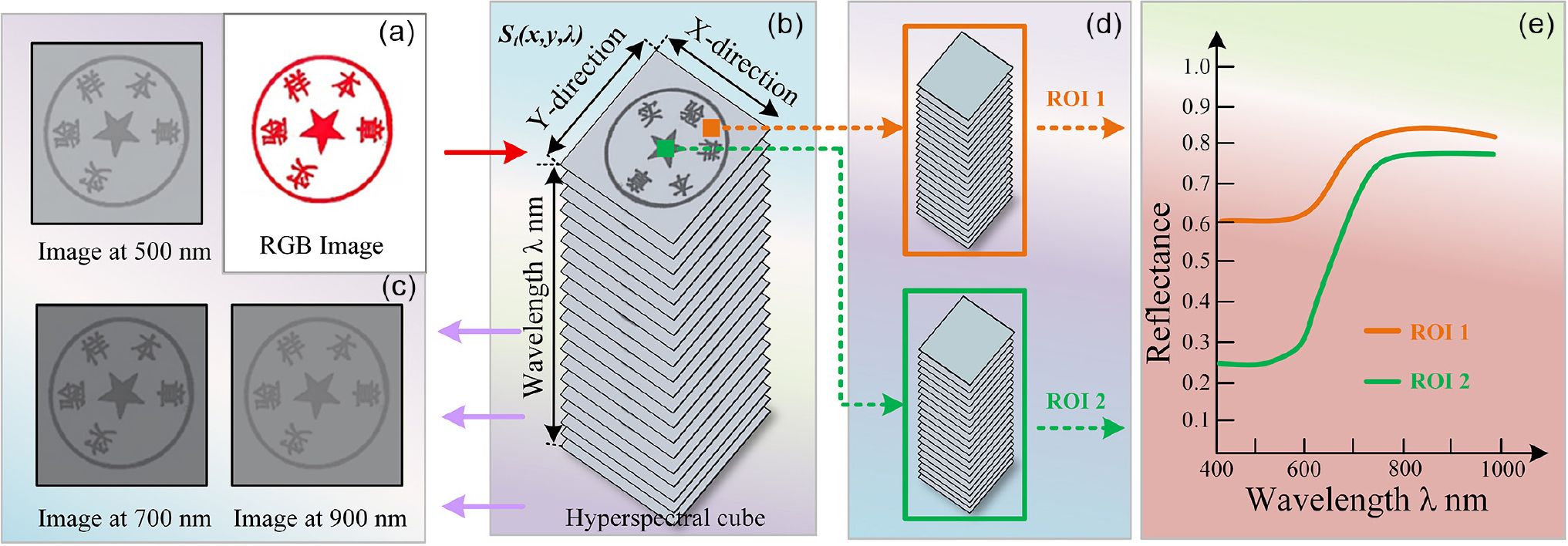
Figure 1 illustrates an example of acquiring hyperspectral cube data of a seal impression. First, an experimental seal is stamped on a blank paper sheet size A4 to serve as the imaging sample I_t, with timing initiated at t = 0 (Figure 1a). The sample is then described according to the defined acquisition time intervals. Subsequently, at any given time point, a hyperspectral device is used to capture the raw hyperspectral cube S_t (x, y, λ) of the imaging sample I_t. The raw hyperspectral cube S_t (x, y, λ) consists of a series of consecutive sub-images I_t ^λ, each acquired at a different wavelength λ in sequential order (Figure 1b). Each sub-image provides the spatial distribution of spectral intensity at a specific wavelength λ. This implies that the dataset described as S_t (x, y, λ) can be interpreted either as individual spatial images S_t (x, y) at each specific wavelength λ, or as spectral curves S_t(λ) at each individual pixel (x,y). Figure 1c illustrates a spatial image extracted from the hyperspectral cube at a specific wavelength within the sensitivity range of the system. The grayscale image reveals varying spectral intensities of the sample at that wavelength due to the distribution of its corresponding chemical components. In Figure 1d, two regions of interest (ROI1 and ROI2) are selected on the hyperspectral image, and the spectral data obtained from these regions are shown in Figure 1e.

Figure 1
Schematic diagram of a hyperspectral image (hyperspectral cube) of a seal impression.

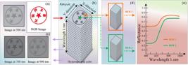
These spectral curves can be regarded as unique spectral fingerprints of the respective pixels, characterizing the composition at those specific locations. Following the workflow outlined in Figure 1, the raw imaging samples at different time points are processed. After continuous long-term acquisition, a collection of hyperspectral cubes is obtained:

(1) $$\mathrm{C}=\left\{{\mathrm{S}}_{\mathrm{t}}\right\},{\mathrm{S}}_{\mathrm{t}}\in {\mathbb{R}}^{\mathrm{X}\times \mathrm{Y}\times \mathrm{B}},\mathrm{t}\in \{{\mathrm{t}}_0,{\mathrm{t}}_1,{\mathrm{t}}_2,\cdots ,{\mathrm{t}}_{\mathrm{N}}\}$$

where C represents the long-term collection of spectral cubes, and S_t denotes the hyperspectral cube of the initially prepared sample at time t. It is important to note that the acquisition time intervals are randomized.

In practical applications, a hyperspectral imaging system must undergo a series of calibration steps to obtain accurate and reliable data. First, the system scans a standard calibration lamp under controlled conditions, and its spectral peaks are mathematically aligned with a standardized spectral axis to complete spectral calibration of the system. This process is critical and must be repeated if the physical layout of the system changes or components are reassembled. Calibration typically needs to be performed multiple times to assess the stability and reproducibility of the system under different operating conditions. Once spectral calibration is completed, the system can be used to acquire hyperspectral images of samples. However, prior to formal analysis, a crucial reflectance calibration step must be executed. This step aims to eliminate background noise and dark current effects inherent to the instrument. Specifically, it is achieved by acquiring two reference images: first, imaging a highreflectance standard white board W_λ to establish the reflectance baseline; second, capturing an image D_λ under complete light-blocking conditions to obtain the inherent dark of the camera current signal. Only after completing this comprehensive calibration process can the spectral data extracted from sample images possess genuine physical significance and research value. Using these two reference images, the pixel-based relative reflectance of the raw line-scan image is calculated with the following formula:³²

(2) $${\rho }_{\lambda }=\frac{{\mathrm{R}}_{\lambda }-{\mathrm{D}}_{\lambda }}{{\mathrm{W}}_{\lambda }-{\mathrm{D}}_{\lambda }}$$

where r_λ is the relative reflectance image, R_λ is the raw reflectance image, D_λ is the dark reference image, and W_λ is the white reference image.

The corrected hyperspectral image can also be expressed in terms of absorbance (A) by applying the following formula derived from the equation:

(3) $$\mathrm{A}=-{\log }_{10}\left(\frac{{\mathrm{R}}_{\lambda }-{\mathrm{D}}_{\lambda }}{{\mathrm{W}}_{\lambda }-{\mathrm{D}}_{\lambda }}\right)$$

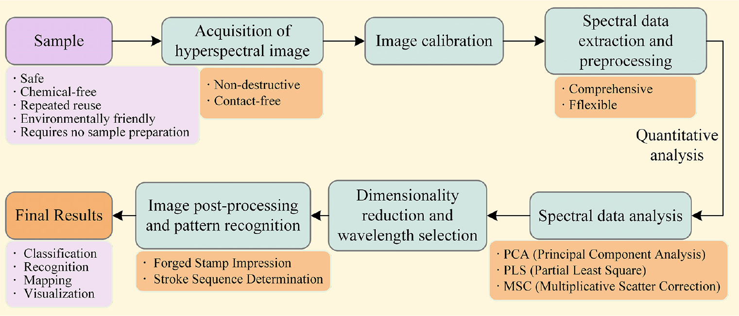
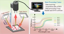
After acquiring the hyperspectral image of the test sample, it should be calibrated using the previously mentioned white and dark reference hyperspectral images. Spectral data are then extracted from different ROIs within the calibrated image that exhibit distinct quality characteristics. Preprocessing techniques such as MSC, standard normal variate (SNV) transformation, Savitzky-Golay (SG) convolution smoothing, and principal component analysis (PCA) are applied to the hyperspectral data to suppress noise and provide a robust foundation for subsequent modeling. Subsequently, these data are utilized for training and testing machine learning models to achieve rapid forensic identification of physical evidence.¹⁶ Currently, the systematic calibration of hyperspectral imaging systems, spectral data extraction and preprocessing, as well as multivariate analysis functions, have been integrated into a software package. This enables professional researchers to execute each key step of these processes through a graphical user interface (GUI). Figure 2 illustrates the critical workflow of hyperspectral data acquisition and highlights the advantages of hyperspectral imaging technology in the authentication of seal impressions:³³ (i) no sample preparation required: HSI is a chemical-free evaluation method that ensures safety and environmental protection by completely eliminating the use of contaminating solvents, chemicals, and/or potentially hazardous reagents during the analysis process; (ii) non-contact, non-invasive, and non-destructive: the method eliminates the need for chemical reagent extraction, dissolution, or physical detachment of the material under examination, thereby avoiding any physical or chemical damage to the seal impression or paper substrate. This fully preserves the original state of the evidence, allowing for multiple rounds of imaging analysis under varied conditions using the same sample; (iii) comprehensiveness and flexibility: HIS acquires a three-dimensional data cube of the sample, which records a spectral volume containing the complete spectrum of each point (pixel) within the sample. This allows for the selection of any ROI in the image for analysis; (iv) capability to discern subtle differences: HIS distinguishes between metameric substances based on their distinct absorption and reflection characteristics across different spectral bands (particularly in the nearinfrared region). It can differentiate inks with varying chemical compositions such as oil-based stamp ink, photosensitive ink, and cinnabar seal paste and determine the sequence of stamp applications; (v) penetration and separation capability: by selecting specific spectral bands, the system can effectively eliminate background interference, detect alterations and forgeries, and identify residual, visually imperceptible original toner or ink components, thereby revealing fraudulent manipulations.

Figure 2
Flowchart of the key steps involved in hyperspectral imaging analysis.

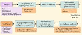
Based on the above advantages, this study employs hyperspectral imaging technology to capture the spectral fingerprints of test samples by detecting changes in their chemical composition over time, thereby providing data support for predicting the age of seal impressions.

Predictor

This study selects SVM as the predictor. The SVM algorithm was proposed in 1964 and underwent rapid development with numerous extensions and improvements between 1992 and 1995, demonstrating high applicability in classification or regression analysis problems across different domains.³⁴ Support vector regression (SVR) is an extension of SVM to regression problems. Its core concept differs from that of SVM, which seeks a maximum-margin hyperplane to separate two classes of samples. Instead, SVR aims to find a tube (or ε-insensitive band). SVR employs a specific loss function known as the ε-insensitive loss function. For a single sample point (X_i, y_i), the loss (L_∈) is defined as:

(4) $${\mathrm{L}}_{ϵ}({\mathrm{y}}_{\mathrm{i}},\mathrm{f}\left({\mathrm{X}}_{\mathrm{i}}\right))=max(0,|{\mathrm{y}}_{\mathrm{i}}-\mathrm{f}\left({\mathrm{X}}_{\mathrm{i}}\right)|-ϵ)$$

(5) $$\mathrm{f}(\mathrm{X})=\mathrm{w}\times \mathrm{X}+\mathrm{b}$$

where X is the feature vector of an input sample, w is the weight vector, b is the bias term, and f(X) is the predicted value for the input sample X. SVR does not require all points to lie exactly on the fitted line; instead, it allows a tolerance deviation ε. Data points falling within this tube incur no loss; only points outside the tube are penalized by having their loss calculated:

(6) $$\{\begin{array}{l}|{\mathrm{y}}_{\mathrm{i}}-f\left({\mathrm{x}}_{\mathrm{i}}\right)|\le ϵ,{\mathrm{L}}_{ϵ}=0\\ |{\mathrm{y}}_{\mathrm{i}}-f\left({\mathrm{x}}_{\mathrm{i}}\right)|>ϵ,L_{ϵ}=|{\mathrm{y}}_{\mathrm{i}}-f\left({\mathrm{x}}_{\mathrm{i}}\right)|-ϵ\end{array}$$

Similar to the classification problem in SVM, the optimization objective of SVR is to minimize both the model complexity and the total deviation beyond the ε-tube. By introducing two slack variables, ξ_i and ξ_i^*, which represent the degrees of deviation above and below the tube respectively, the primal optimization problem can be formulated as follows:

(7) $$\begin{array}{rl}& \underset{\mathrm{w},\mathrm{b},\xi ,{\xi }^{\ast }}{max}\frac{1}{2}\Vert \mathrm{w}{\Vert }^2+\mathrm{C}\sum _{\mathrm{i}=1}^{\mathrm{n}}({\xi }_i+{\xi }_i^{\ast })\\ & \text{s.t.}\{\begin{array}{c}{\mathrm{y}}_{\mathrm{i}}-(\mathrm{w}\times {\mathrm{X}}_{\mathrm{i}}+\mathrm{b})\le ϵ+{\xi }_{\mathrm{i}}\\ (\mathrm{w}\times {\mathrm{X}}_{\mathrm{i}}+\mathrm{b})-{\mathrm{y}}_{\mathrm{i}}\le ϵ+{\xi }_{\mathrm{i}}^{\ast }\\ {\xi }_{\mathrm{i}},{\xi }_{\mathrm{i}}^{\ast }\ge 0\end{array}\end{array}$$

where $\frac{1}{2}\Vert \mathrm{w}{\Vert }^2$ represents the flatness of the model, the 2 smaller its value, the flatter the model. C is the penalty parameter, which controls the tolerance for samples that deviate beyond the tube. A larger C makes the model less tolerant to deviation, potentially leading to overfitting; a smaller increases the tolerance of the model, which may result in underfitting. The term $C\sum _{i=1}^n({\xi }_i+{\xi }_i^{\ast })$ denotes the total penalty imposed on samples that exceed the ε-tube. ε defines the width of the tube. A larger results in a wider tube, fewer support vectors, and a simpler model; a smaller ∈ imposes stricter fitting accuracy requirements, potentially leading to a more complex model.

Evaluation metrics

In this study, the accuracy of the developed method was evaluated based on commonly used performance.³⁵ The coefficient of determination (R²) and the root mean square error (RMSE) are two of the most widely adopted evaluation metrics for assessing the performance of spectral analysis models.¹⁷ In addition, metrics such as mean absolute percentage error (MAPE), mean absolute error (MAE), Kling-Gupta efficiency (KGE) and Nash-Sutcliffe efficiency (NSE) can also be used to evaluate prediction performance.³⁰,³¹ The coefficient of determination quantifies the strength of the linear relationship between model-predicted values and actual observed values, while RMSE measures the average magnitude of prediction errors between predicted and true values. To objectively evaluate the reliability and generalization ability of a model, performance assessment should be conducted based on an independent test set or randomly generated samples using techniques such as cross-validation. The formulas for calculating R², RMSE, MAPE, MAE, NSE and KGE are as follows:

(8) $${\mathrm{R}}^2=1-\frac{\sum _{\mathrm{i}=1}^{\mathrm{n}}{({\mathrm{y}}_{\mathrm{p},\mathrm{i}}-{\bar{\mathrm{y}}}_{\mathrm{o},\mathrm{i}})}^2}{{\mathrm{y}}_{\mathrm{o},\mathrm{i}}^2},0\le {\mathrm{R}}^2\le 1$$

(9) $$\mathrm{RMSE}=\sqrt{\frac{1}{\mathrm{n}}\sum _{\mathrm{i}=1}^{\mathrm{n}}{({\mathrm{y}}_{\mathrm{o},\mathrm{i}}-{\mathrm{y}}_{\mathrm{p},\mathrm{i}})}^2}$$

(10) $$\mathrm{MAPE}(\mathrm{\%})=\frac{1}{\mathrm{n}}\sum _{\mathrm{i}=1}^{\mathrm{n}}\left|\frac{{\mathrm{y}}_{\mathrm{o},\mathrm{i}}-{\mathrm{y}}_{\mathrm{p},\mathrm{i}}}{{\mathrm{y}}_{\mathrm{o},\mathrm{i}}}\right|\times 100$$

(11) $$\mathrm{MAE}=\frac{1}{\mathrm{n}}\sum _{\mathrm{i}=1}^{\mathrm{n}}|{\mathrm{y}}_{\mathrm{p},\mathrm{i}}-{\mathrm{y}}_{\mathrm{o},\mathrm{i}}|$$

(12) $$\mathrm{NSE}=1-\frac{\sum _{\mathrm{i}=1}^{\mathrm{n}}{({\mathrm{y}}_{\mathrm{p},\mathrm{i}}-{\mathrm{y}}_{\mathrm{o},\mathrm{i}})}^2}{\sum _{\mathrm{i}=1}^{\mathrm{n}}{({\mathrm{y}}_{\mathrm{o},\mathrm{i}}-{\bar{\mathrm{y}}}_{\mathrm{o}})}^2}\to -\mathrm{\infty }\le \mathrm{NSE}\le 1$$

(13) $$\mathrm{KGE}=1-\sqrt{(\mathrm{r}-1{)}^2+{(\frac{{\sigma }_{\mathrm{p}}}{{\sigma }_{\mathrm{o}}}-1)}^2+{(\frac{{\bar{\mathrm{y}}}_{\mathrm{p}}}{{\bar{\mathrm{y}}}_{\mathrm{o}}}-1)}^2}$$

where n represents the sample size, y_o denotes the observed sample, y_p is the predicted value, y_o is the mean value of the samples, σ_o and σ_p and are the standard deviations of the observed and predicted values, respectively, and r in equation 13 is the Pearson correlation coefficient.

Based on the above metrics, we propose a composite indicator specifically designed to diagnose whether a model is overfitting, which quantifies the degradation or gap in model performance between the training set and the test set. A robust, non-overfitted model should exhibit similar performance on both sets, whereas an overfitted model will demonstrate a significant performance gap.

(14) $$r_{\mathrm{dR}}(\mathrm{\%})=\left|\frac{{\mathrm{NSE}}_1^2-{\mathrm{NSE}}_2^2}{{\mathrm{NSE}}_1^2}\right|\times 100$$

In the equation, NSE₁² and NSE²₂ represent the Nash-Sutcliffe efficiency of the training set and test set, respectively. The metric quantifies the rate of performance degradation. A lower index value (closer to 0) indicates a more robust model.

Data acquisition

Acquisition equipment

In this study, a hyperspectral imaging system produced by Shenzhen Zhongda Ruihe Technology Co., Ltd. was employed to collect spectral data from seal impression samples. The system primarily consists of the following core components: a hyperspectral imager based on liquid crystal tunable filter (LCTF) technology, equipped with a 2048 × 2046-pixel CMOS sensor and a 35 mm aperture optical system; an adjustable sample stage; and four sets of halogen broadband white-light source arrays (color temperature 3200 ± 100K). The operating spectral range of the system covers 400-1000 nm (visible to near-infrared region), with a spectral resolution of 5 nm and a spatial resolution of 2048 × 2046 pixels. The exposure time was fixed at 40 ms, and data acquisition was performed in pushbroom scanning mode. During the data acquisition process, the following standardized procedures were strictly adhered to: first, a 10-min system warm-up was conducted to ensure light source stability; second, radiation calibration using a standard white board and dark current correction were performed in an enclosed environment; finally, full-band data of the samples were acquired under fixed conditions, including a sample stage height of 50 ± 1 cm and a light source incident angle of 45 ± 2°.

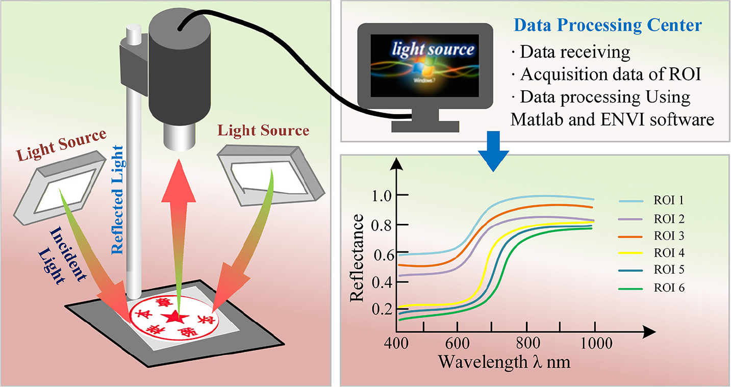
Data processing was carried out using a collaborative workflow between ENVI 5.6 (Exelis Visual Information Solutions, Harris Corporation, Broomfield, Colorado, USA, 2020) software and MATLAB 2023a (MathWorks, Natick, MA, USA, 2023). The former was primarily employed for ROI selection, spectral curve visualization, and spatial-spectral joint analysis; the latter was responsible for image cube preprocessing, spectral feature extraction, and algorithm implementation. Figure 3 illustrates a detailed schematic diagram of the hyperspectral imaging system configuration, including the optical layout and spatial arrangement of its components. Through the precise wavelength-tuning mechanism of the LCTF combined with the high-sensitivity CMOS sensor, the system achieves high-precision and high-stability spectral image acquisition.

Figure 3
Schematic diagram of the detailed configuration of the hyperspectral imaging system.

Data acquisition and processing

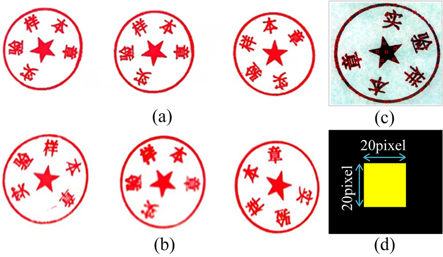
This study selected oil-based stamp inks from two brands as experimental materials, with A4 copy paper (basis weight 80 g m^-2) serving as the printing substrate. Sample preparation was carried out using an HP LaserJet 2606dw laser printer (resolution 1200 × 1200 dpi). The experiment utilized two new, unused 38 mm oil-based seals, each filled with one brand of ink. Under strictly controlled and consistent stamping conditions, each seal was pressed three times consecutively on A4 copy paper (all stamping operations were uniformly completed at 09:50 on November 17, 2024), resulting in hyperspectral images of six seal impressions per time point. After all samples were prepared, they were left undisturbed for 10 h in a constant temperature and humidity environment (25 °C, 35% relative humidity) to ensure complete ink curing, thereby providing standardized and highly reproducible experimental samples for subsequent analysis. Hyperspectral data were subsequently collected from each seal impression sample at 27-time intervals as listed in Table 1. During spectral image processing, the ROI function in ENVI software was used to manually delineate a 20 × 20-pixel detection area on each seal impression sample, as shown in Figure 4. ROIs were extracted from the same stamp impression, all ROIs were located within uniform ink-distribution areas of valid impressions, avoiding edges and defective regions. By calculating the average spectral value within each ROI, spectral feature data were extracted for each sample (see Figure 4 for an example, which illustrates sample 1 of a stamp impression at a 0.42-day interval along with a schematic of its ROI selection). Using the ROI function in ENVI software, we manually delineated a 20 × 20-pixel detection area on each seal impression sample (Figures 4c and 4d). All ROIs were positioned within the valid impression area where ink distribution was uniform, avoiding edges and defective regions. During data processing, we first constructed separate datasets for the two ink brands. Samples 1 and 2 were used as the training set, with 20 ROI regions selected from each hyperspectral data of the sample as training spectral data, resulting in a total of 1,080 spectral data points for the two training samples (27 time points × 20 ROIs × 2 samples = 1,080). Sample 3 served as the test set, with 20 ROI regions similarly selected as test spectral data, yielding a total of 540 spectral data points (27 time points × 20 ROIs = 540). The average spectral value within each ROI was calculated to extract the spectral feature data for each sample (see Figure 4 for an example, which illustrates sample 1 of a stamp impression at a 0.42day interval along with a schematic of its ROI selection).

Table 1
Sampling intervals for spectral data of each sample

Sample Dataset	Intervals / days			Number of intervals	Spectral data per interval	Total spectral data per dataset
Sample 1 training Sample 2	0.42, 7.5, 21.25, 22.43, 28.47, 32.43, 41.17, 46.42, 48.06, 54.05, 62.18, 69.02, 70.02, 76.21, 84.08, 92.02, 105.08, 112.7, 119.2, 125.32, 132, 135, 140, 148, 162, 182, 205			27	40		1080
Sample 3 test	0.42, 7.5, 21.25, 22.43, 28.47, 32.43, 41.17, 46.42, 48.06, 54.05, 62.18, 69.02, 70.02, 76.21, 84.08, 92.02, 105.08, 112.7, 119.2, 125.32, 132, 135, 140, 148, 162, 182, 205			27	20		540

Figure 4
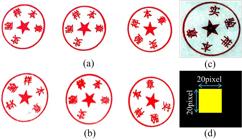
Schematic diagram of sample 1 and its regions of interest (ROI) selection. (a) and (b) different stamp pad inks, (c) ROI setup, (d) ROI of (c).

Results and Discussion

Preprocessing and model setup

This study employs SVM, ELM, PLS, BP, and LSTM as predictors. These models were trained using the preprocessed hyperspectral training set, and their performance was evaluated on the test set. The parameter settings for the machine learning methods are provided in Table 2 to facilitate reproducibility of our research by other scholars.

Table 2
Parameter settings for machine learning models

Model		Parameter	Value		Description
SVR		Kernal p RBF	RBF 0.01 2		Kernal function Epsilon value Kernel size
		c	4		cost
		g	4		Kernal width
ELM		q Activation function	100 sigmoid		number of hidden neurons sigmoidal function
PLS		km kb	30 21		max value of K best value of K
BP		S epochs goal	5 500 1 × 104		sizes of N-1 hidden layers number of iterations error threshold
		Lr	0.01		learning rate
LSTM		Hidden units Optimizer Activation function Epochs	121 adam Relu 1500		the number of hidden units parameter optimizer for training activation function maximum number of trainings
		Learning rate	0.005		initial rearn rate
		Drop factor	0.1		learning rate decline factor
		Drop period	1400		decreased after 1400 training sessions

In raw spectral data, both effective sample information and noise interference are present. Therefore, the preprocessing step plays a critical role in suppressing noise and enhancing subsequent modeling performance. The preprocessing methods including MSC, SNV, and Savitzky-Golay are applied separately to the training and testing datasets, along with SVM, LSTM, PLS, BP, and ELM predictors, to construct estimation models for stamp impression age. MSC and SNV both belong to scatter correction methods, aiming to reduce non-target variability caused by light scattering and enhance the effective information components in the spectra. SNV is functionally similar to MSC and can be used to eliminate errors in individual spectra due to sample surface scattering. Additionally, Savitzky-Golay smoothing is primarily used to compress baseline drift and highlight spectral features, thereby improving spectral resolution. The results indicate that MSC, by correcting the scattering effects in individual spectra, can significantly attenuate interference caused by scattering, effectively extracting more accurate spectral absorption features, and demonstrates superior noise suppression and signal enhancement among various preprocessing methods. The parameter settings for SVM, LSTM, BP, PLS, and ELM are detailed in Table 2.

Table 3 presents the performance classification criteria for four key evaluation metrics used in this study: the coefficient of determination (R²), Nash-Sutcliffe efficiency coefficient (NSE), Kling-Gupta efficiency (KGE), and rate of performance degradation (r_dR). For R² and NSE, values closer to 1 indicate better model performance, with a five-tier classification system ranging from unsatisfactory (≤ 0.40) to very good (≥ 0.90 for R²; ≥ 0.80 for NSE). The KGE metric follows a similar progressive scale, where values above 0.70 are considered very good, while those below 0.40 are deemed unsatisfactory. Notably, the metric, which measures the relative difference between training and testing R², employs an inverse classification: lower values indicate better model stability and generalization, with r_dR ≤ 5 classified as good and values exceeding 30 considered unsatisfactory. This comprehensive evaluation framework enables a nuanced assessment of both predictive accuracy and model robustness across different preprocessing techniques and machine learning algorithms.

Table 3
Range of evaluation metrics and performance, including R², NSE, KGE and r_dR

Range of NSE	Performance	Range of KGE	Performance
NSE ≤ 0.40	unsatisfactory	KGE ≤ 0.40	unsatisfactory
0.40 < NSE ≤ 0.60	acceptable	0.40 < KGE ≤ 0.50	acceptable
0.60 < NSE ≤ 0.80	satisfactory	0.50 < KGE ≤ 0.60	satisfactory
0.80 < NSE ≤ 0.90	good	0.60 < KGE ≤ 0.70	good
0.90 < NSE ≤ 1.00	very good	0.70 < KGE ≤ 1.00	very good
Range of R2	performance	range of rdR	performance
R2 ≤ 0.40	unsatisfactory	rdR > 25	unsatisfactory
0.40 < R2 ≤ 0.60	regular	15 < rdR ≥ 25	regular
0.60 < R2 ≤ 0.80	good	5 < rdR ≥ 15	satisfactory
0.80 < R2 ≤ 1.00	very good	0 < rdR ≥ 5	good

Results on 10-fold cross-validation

We performed 10-fold cross-validation experiments, the results for five machine learning algorithms (ELM, PLS, BP, LSTM, and SVM) combined with four preprocessing techniques (raw, SG, SNV, and MSC) as shown in Tables 4-7. The results of 10-fold cross-validation show that: (i) SVM demonstrated superior performance across all preprocessing techniques, particularly when combined with MSC, achieving the highest NSE values (ranging from 0.97 to 0.99) and lowest RMSE (4.85-10.09). The exceptional stability of SVM is evidenced by the narrow performance range across the 10 folds, suggesting excellent generalization capability. LSTM and BP also exhibited competitive performance, with MSC-preprocessed LSTM achieving NSE values between 0.91 and 0.96 and RMSE between 10.57 and 16.32. However, BP displayed notable sensitivity to preprocessing, with SNV leading to severe performance degradation in certain folds (e.g., fold 4 NSE = 0.32). ELM and PLS showed moderate but relatively stable performance, with PLS demonstrating particular robustness to different preprocessing techniques; (ii) the MSC preprocessing technique consistently yielded the most robust and accurate predictions across all algorithms, with substantially higher NSE values and lower RMSE compared to other preprocessing methods. In contrast, SNV preprocessing resulted in the poorest overall performance, characterized by highly variable NSE values and elevated RMSE across most algorithms, indicating its limited effectiveness in enhancing model generalization for this application; (iii) the SVM-MSC combination demonstrated exceptional stability, with minimal foldto-fold variation in both NSE (standard deviation < 0.01) and RMSE (standard deviation < 1.5). This consistency underscores its reliability for practical forensic applications. In contrast, SNV-preprocessed models exhibited high variability, particularly for BP (NSE ranging from 0.32 to 0.96 across folds) and ELM (NSE ranging from 0.42 to 0.73), indicating poor model robustness.

Table 4
Ten-fold cross-validation results of different ML algorithms (ELM, PLS, BP, LSTM, SVM) under different preprocessing techniques (raw)

K	NSE					RMSE
	ELM	PLS	BP	LSTM	SVM	ELM	PLS	BP	LSTM	SVM
1	0.68	0.75	0.80	0.85	0.87	29.48	26.26	23.23	19.98	19.04
2	0.77	0.81	0.89	0.92	0.91	25.96	23.63	17.75	15.05	15.83
3	0.77	0.84	0.90	0.90	0.88	27.31	23.18	17.93	18.40	19.82
4	0.72	0.80	0.88	0.89	0.87	28.81	24.10	18.86	18.39	19.65
5	0.84	0.87	0.93	0.93	0.88	22.30	20.35	14.44	14.59	19.49
6	0.75	0.81	0.88	0.90	0.87	24.61	21.38	17.21	15.31	17.57
7	0.71	0.82	0.89	0.92	0.91	28.96	22.96	17.75	15.63	16.36
8	0.80	0.81	0.92	0.92	0.90	25.11	24.21	15.98	16.12	17.48
9	0.73	0.86	0.90	0.91	0.91	28.19	20.28	17.15	16.57	16.03
10	0.76	0.82	0.90	0.89	0.84	28.50	24.48	18.51	19.58	23.24
Mean	0.753	0.81	0.88	0.90	0.88	26.92	23.08	17.88	16.96	18.45

Table 5
Ten-fold cross-validation results of different ML algorithms (ELM, PLS, BP, LSTM, SVM) under different preprocessing techniques (SG)

K	NSE					RMSE
	ELM	PLS	BP	LSTM	SVM	ELM	PLS	BP	LSTM	SVM
1	0.69	0.76	0.86	0.85	0.86	29.04	25.57	19.60	20.37	19.88
2	0.80	0.83	0.88	0.91	0.90	23.99	22.13	18.68	16.35	16.88
3	0.76	0.83	0.86	0.90	0.87	28.12	23.23	21.70	17.72	20.56
4	0.70	0.78	0.87	0.87	0.86	29.65	25.21	19.70	19.67	20.22
5	0.84	0.82	0.92	0.90	0.87	22.08	23.30	15.60	17.42	19.99
6	0.75	0.77	0.88	0.89	0.86	24.44	23.70	16.86	16.37	18.33
7	0.78	0.79	0.91	0.88	0.90	25.49	24.45	16.56	18.90	17.13
8	0.81	0.81	0.89	0.91	0.89	24.12	24.07	18.30	16.27	18.29
9	0.74	0.83	0.86	0.90	0.90	27.94	22.30	20.10	16.76	17.46
10	0.70	0.80	0.79	0.88	0.82	31.69	26.23	26.62	20.57	24.60
Mean	0.75	0.80	0.87	0.88	0.87	26.65	24.01	19.37	18.04	19.33

Table 6
Ten-fold cross-validation results of different ML algorithms (ELM, PLS, BP, LSTM, SVM) under different preprocessing techniques (SNV)

K	NSE					RMSE
	ELM	PLS	BP	LSTM	SVM	ELM	PLS	BP	LSTM	SVM
1	0.64	0.55	0.67	0.70	0.92	31.48	35.15	30.07	28.66	14.49
2	0.61	0.65	0.84	0.72	0.95	33.53	31.60	21.76	28.26	12.41
3	0.62	0.54	0.76	0.74	0.95	35.19	38.86	28.23	29.27	12.82
4	0.64	0.55	0.32	0.75	0.94	32.62	36.30	44.83	27.20	13.77
5	0.71	0.68	0.90	0.72	0.94	29.72	31.39	17.63	29.52	13.24
6	0.43	0.60	0.69	0.61	0.92	37.28	31.21	27.35	30.84	13.85
7	0.59	0.64	0.92	0.74	0.93	34.66	32.51	14.99	27.47	14.45
8	0.73	0.64	0.96	0.78	0.94	29.13	33.23	11.54	26.37	13.92
9	0.62	0.73	0.92	0.78	0.96	33.61	28.03	15.06	25.68	10.89
10	0.42	0.53	0.83	0.69	0.91	44.16	39.91	23.86	32.51	17.61
Mean	0.60	0.61	0.78	0.72	0.93	34.13	33.81	23.53	28.57	13.74

Table 7
Ten-fold cross-validation results of different ML algorithms (ELM, PLS, BP, LSTM, SVM) under different preprocessing techniques (MSC)

K	NSE					RMSE
	ELM	PLS	BP	LSTM	SVM	ELM	PLS	BP	LSTM	SVM
1	0.77	0.73	0.91	0.91	0.98	25.33	27.25	15.61	15.99	7.41
2	0.82	0.80	0.95	0.95	0.98	22.93	23.93	11.77	12.19	7.78
3	0.80	0.85	0.95	0.93	0.98	25.44	22.45	13.28	14.77	7.87
4	0.78	0.80	0.93	0.93	0.98	25.55	24.33	14.79	14.05	6.80
5	0.89	0.86	0.97	0.94	0.98	18.36	20.58	9.50	13.13	6.85
6	0.76	0.80	0.90	0.93	0.98	24.04	21.87	15.79	13.32	6.47
7	0.82	0.81	0.97	0.94	0.99	22.85	23.52	9.23	13.14	4.85
8	0.85	0.81	0.97	0.96	0.99	21.75	24.44	10.39	10.57	6.30
9	0.80	0.85	0.93	0.95	0.97	24.18	20.81	13.93	12.04	9.36
10	0.84	0.83	0.95	0.92	0.97	23.57	24.25	13.51	16.32	10.09
Mean	0.81	0.81	0.94	0.93	0.98	23.4	23.34	12.78	13.55	7.37

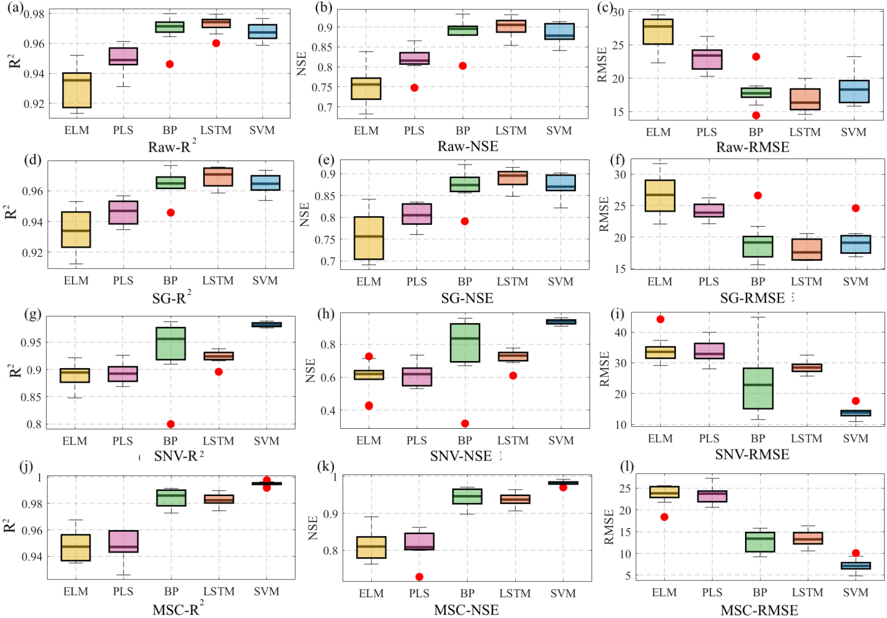
Figure 5 presents boxplots of 10-fold cross-validation results across five machine learning algorithms (ELM, PLS, BP, LSTM, and SVM) combined with four preprocessing techniques (raw, SG, SNV, and MSC), evaluated using R², NSE and RMSE. As shown in Figure 5, outliers are denoted by red dots. The median line of the box of BP is shifted toward the upper quartile, accompanied by an upper whisker shorter than the lower whisker, which is indicative of a right-skewed distribution. Furthermore, the relatively tall boxes for ELM and BP reflect considerable variability in their predictions, whereas the notably shorter box for SVM attests to its superior stability.

Figure 5
Boxplots of 10-fold cross-validation results under different combination modes. R²: coefficient of determination; NSE: Nash-Sutcliffe efficiency; RMSE: root mean square error; SG: Savitzky-Golay; SNV: standard normal variate; MSC: multiplicative scatter correction.

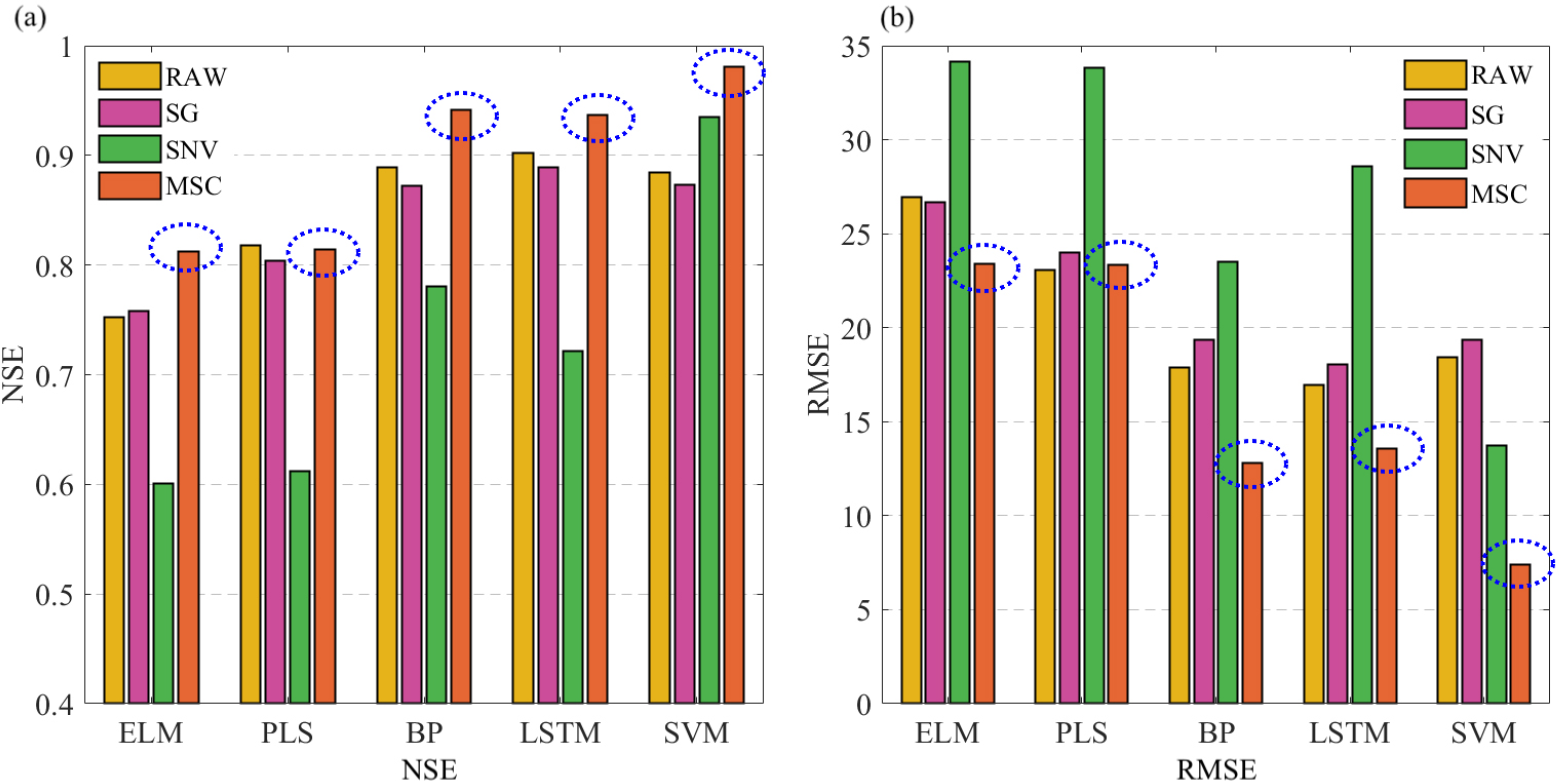
Figure 6 reveals distinct performance patterns across algorithms and preprocessing techniques. SVM consistently achieves the highest average NSE (0.98) and lowest average RMSE (7.37) across all preprocessing methods, demonstrating its superior predictive capability. In contrast, ELM exhibits the poorest performance, with NSE values ranging from 0.75 to 0.88 and RMSE values consistently above 16.0, indicating limited effectiveness for stamp age prediction. MSC preprocessing substantially improves model performance across all algorithms, most notably for SVM, where RMSE decreases from 23.39 (raw) to 7.37 (MSC), a 68.49% reduction. For ELM and BP, MSC also yields the highest NSE values (0.81 and 0.94, respectively) and lowest RMSE values (23.39 and 12.78).

Figure 6
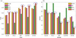
Average performance of 10-fold cross-validation across five machine learning algorithms with four preprocessing techniques. NSE: NashSutcliffe efficiency; RMSE: root mean square error; ELM: extreme learning machine; PLS: partial least-squares; BP: backpropagation neural; LSTM: long short-term memory; SVM: support vector machine. The dotted circle indicates the area where we achieved a higher NSE value and a lower RMSE value, representing the best model performance.

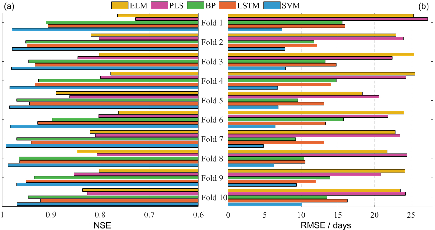
Figure 7 presents the average 10-fold cross-validation performance of five machine learning algorithms following MSC preprocessing, which was identified as the optimal preprocessing technique in the previous analysis.

Figure 7
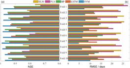
10-fold cross-validation performance based on MSC preprocessing, showing NSE and RMSE distributions for each algorithm. NSE: Nash-Sutcliffe efficiency; RMSE: root mean square error; ELM: extreme learning machine; PLS: partial least-squares; BP: backpropagation neural; LSTM: long shortterm memory; SVM: support vector machine.

Based on the comprehensive evaluation of both NSE and RMSE, the algorithms can be ranked as follows: SVM > BP ≈ LSTM > PLS > ELM. SVM not only achieves the highest accuracy but also demonstrates the greatest robustness to different preprocessing techniques. BP and LSTM show similar performance profiles, with NSE values around 0.93 and RMSE between 12.0-23.0, though LSTM slightly outperforms BP under MSC preprocessing. PLS maintains moderate performance with NSE of 0.80-0.82 and RMSE of 23.0-33.0, while ELM consistently underperforms across all metrics. SVM algorithm combined with MSC preprocessing emerges as the optimal configuration, achieving the highest mean NSE (0.98) and lowest mean RMSE (7.38) with exceptional stability. This configuration significantly outperforms all other combinations, providing strong evidence for its suitability as the primary modeling approach for stamp age prediction.

Results on full dataset

After establishing the optimal configurations through 10-fold cross-validation, we conducted comprehensive experiments on the entire dataset to assess the final predictive performance and generalization ability of the selected models. These experiments utilize all available samples for training and testing, providing a holistic evaluation of model effectiveness under real-world application scenarios.

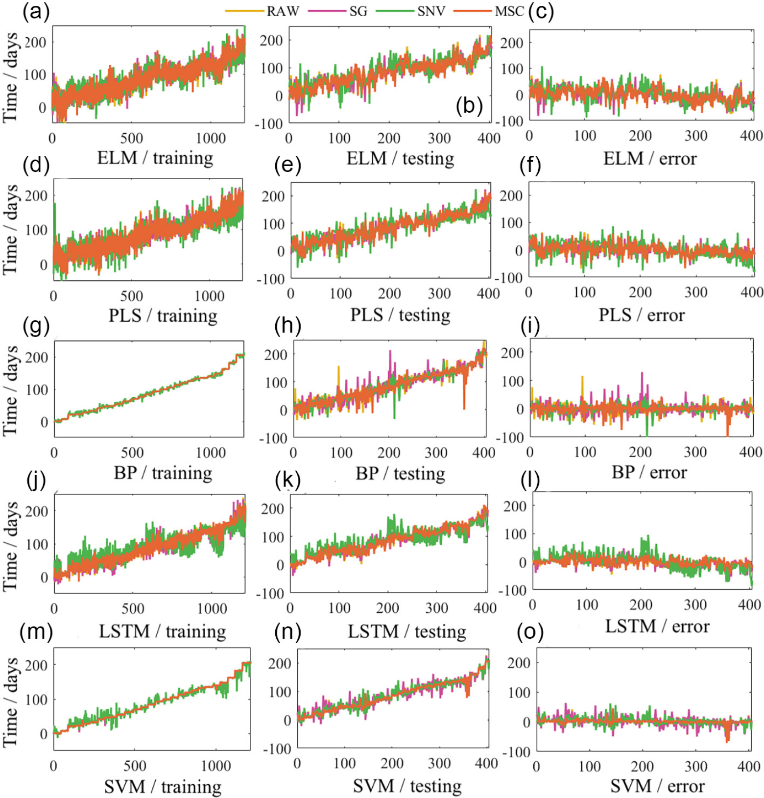
The dataset was split into training and test sets in a 3:1 ratio. The results of different processing methods and predictors on the training and test sets are shown in Figure 8. To facilitate clearer visualization, the y-axis range was kept fixed across plots. Figures 8a, 8d, 8g, 8j, 8m displays the predicted values of different methods (SVM, LSTM, PLS, ELM, BP) on the training set, with distinct colors representing different preprocessing methods. Figures 8b, 8e, 8h, 8k, 8n show the predicted values of these methods on the test set. Figures 8c, 8f, 8i, 8l, 8o presents the deviation between true and predicted values on the test set. The results indicate that, regardless of the preprocessing method used, SVM consistently achieves the best performance on the training set, while other methods exhibit larger fluctuations in predicted values. BP demonstrated superior performance on the training set; however, its test set errors exceeded those of SVM, indicating that BP is prone to overfitting.

Figure 8
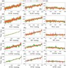
Performance of different methods on the training set and test set. ELM: extreme learning machine; PLS: partial least-squares; BP: backpropagation neural; LSTM: long short-term memory; SVM: support vector machine.

The comprehensive performance evaluation of different machine learning algorithms combined with various preprocessing techniques is presented in Table 8. Raw indicates unprocessed data, serving as a baseline to compare the effects of all preprocessing methods. To comprehensively evaluate the predictive performance of each model, the following metrics were selected: R², NSE, RMSE, MAE, KGE, and r_dR, which collectively assess the ability of the model to explain variance in the target variable: (i) among all evaluated configurations, the MSC preprocessing technique consistently yielded the most balanced and robust predictive performance. Notably, models trained on raw data exhibited severe overfitting, particularly BP and SVM, which achieved perfect training scores (R² = 1.00, NSE = 1.00) but demonstrated substantial performance degradation on test sets, as reflected by elevated r_dR values (16.69 for BP and 19.13 for SVM). This discrepancy indicates poor generalization capability despite exceptional training accuracy; (ii) SVM demonstrated superior overall performance, particularly when combined with MSC preprocessing, achieving test set metrics of R² = 0.99, NSE = 0.98, KGE = 0.98, and a remarkably low r_dR of 4.04. This configuration strikes an excellent balance between predictive accuracy and model stability. BP exhibited the most extreme overfitting behavior across all preprocessing methods, with training R² consistently at 1.00 but test NSE dropping to as low as 0.74 (SNV) and reaching 45.82, indicating poor generalization. ELM and PLS showed moderate but stable performance, with relatively consistent training-testing discrepancies. LSTM demonstrated competitive predictive accuracy (test NSE up to 0.94 with MSC) but displayed variable stability depending on preprocessing; (iii) MSC preprocessing consistently enhanced model generalization, as evidenced by the lowest r_dR values across most algorithms (SVM = 4.04, PLS = 0.94, LSTM = 2.47). SG preprocessing yielded comparable but slightly inferior results to raw data, suggesting limited effectiveness in addressing overfitting. SNV preprocessing led to the poorest overall performance, with elevated errors and reduced test NSE, particularly for ELM and PLS, where test NSE dropped below 0.65; (iv) based on the comprehensive evaluation metrics, the SVM model with MSC preprocessing emerges as the optimal configuration, achieving the highest test R² (0.99), NSE (0.98), and KGE (0.94) while maintaining excellent stability (r_dR = 4.04). The BP-MSC combination also demonstrated strong test performance (R² = 0.99, RMSE = 12.19) but with slightly higher r_dR (10.54), indicating marginally lower stability. PLS with MSC achieved exceptional stability (r_dR = 0.94) but slightly lower predictive accuracy compared to SVM.

Table 8
Results of different methods on the training and testing sets

	ML	Training					Testing
		MAE	RMSE	R2	NSE	KGE
MAE	RMSE	R2	NSE	KGE	rdR
Raw	ELM PLS BP	20.86 16.70 0.00	26.34 20.98 0.00	0.93 0.96 1.00	0.77 0.85 1.00	0.83 0.90 1.00	21.64 16.19 11.36	27.16 20.60 15.47	0.93 0.96 0.98	0.73 0.85 0.91	0.83 0.91 0.92	9.23 1.70 16.69
	LSTM	10.55	14.15	0.98	0.93	0.93	10.64	14.24	0.98	0.93	0.92	1.50
	SVM	1.92	2.04	1.00	1.00	0.99	12.05	16.72	0.97	0.90	0.93	19.13
SG	ELM PLS BP	20.30 16.94 0.01	26.13 21.65 0.01	0.94 0.96 1.00	0.77 0.84 1.00	0.83 0.88 0.99	20.65 16.08 12.26	25.51 20.09 16.04	0.94 0.96 0.97	0.76 0.85 0.91	0.83 0.89 0.89	2.13 2.36 17.89
	LSTM	11.97	16.15	0.98	0.91	0.91	12.28	16.67	0.97	0.90	0.91	3.10
	SVM	2.03	2.49	1.00	1.00	0.99	12.46	17.41	0.97	0.89	0.93	20.57
SNV	ELM PLS BP	24.92 25.57 0.45	30.84 32.14 0.84	0.91 0.90 1.00	0.68 0.65 1.00	0.79 0.73 0.99	25.95 25.85 16.71	32.15 31.38 26.91	0.90 0.90 0.93	0.62 0.64 0.74	0.79 0.77 0.94	16.29 3.85 45.82
	LSTM	19.59	26.67	0.93	0.76	0.80	20.56	27.85	0.92	0.72	0.79	11.56
	SVM	4.41	7.87	0.99	0.98	0.97	9.58	13.68	0.98	0.93	0.95	9.47
MSC	ELM PLS BP	17.16 16.80 0.04	22.02 21.28 0.07	0.95 0.96 1.00	0.84 0.85 1.00	0.88 0.89 0.99	19.42 16.47 8.01	24.64 20.68 12.19	0.94 0.96 0.99	0.78 0.84 0.95	0.86 0.90 0.94	13.58 0.94 10.54
	LSTM	9.11	12.09	0.99	0.95	0.95	9.94	12.89	0.98	0.94	0.95	2.47
	SVM	1.61	1.85	1.00	1.00	0.99	3.82	7.69	0.99	0.98	0.98	4.04

Table 9 presents the Kruskal-Wallis test p-values for comparing the distributions of predicted values from five machine learning models against the observed values on both training and testing datasets. The Kruskal-Wallis test is a non-parametric method used to determine whether significant differences exist among the medians of multiple independent samples.³⁶ A p-value greater than 0.05 indicates that there is no statistically significant difference between the distributions of the model predictions and the observed values. SVM achieves consistently high p-values on both training (p = 0.89) and testing (p = 0.94) sets, demonstrating that its predictions are statistically indistinguishable from the observed values. This confirms the robustness and generalization capability of the MSC-SVM configuration for stamp age prediction. These Kruskal-Wallis test results, combined with the other evaluation metrics (R², RMSE, NSE, KGE), provide strong support for selecting SVM as the optimal model.

Table 9
Kruskal-Wallis test results on the measurement and predicted values (MSC)

Dataset		p-value of Kruskal-Wallis test
	ELM	PLS	BP	LSTM	SVM
Training	0.62	0.57	0.96	0.89	0.89
Testing	0.57	0.79	0.74	0.80	0.94
Distance	0.05	0.22	0.22	0.09	0.05

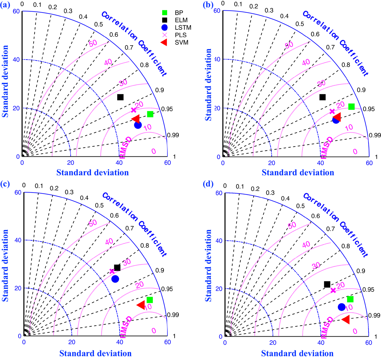
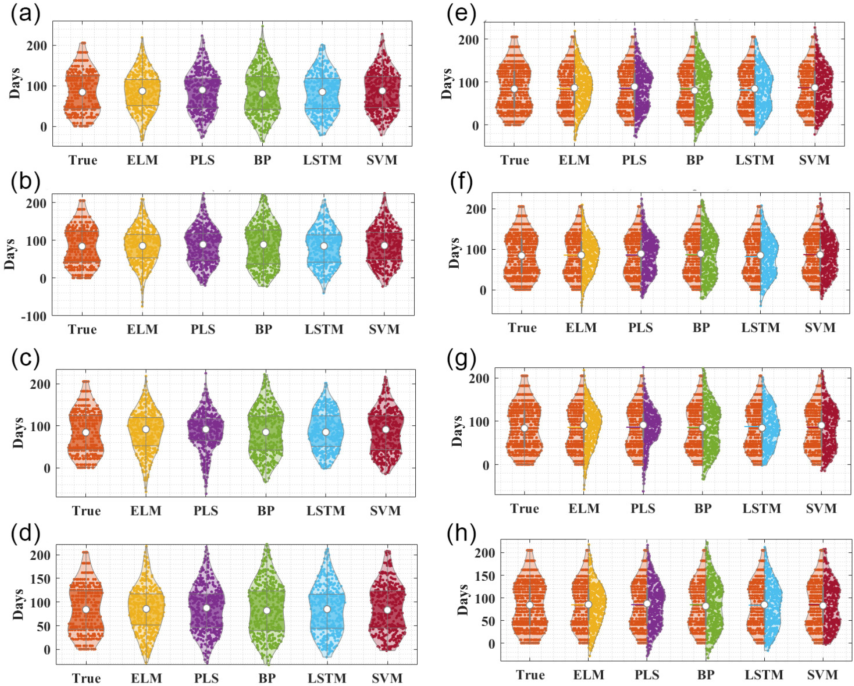
In addition to the overall performance criteria, bar, and time series plots, the performance of the models was evaluated using Taylor and violin diagrams. The results are presented as Taylor and violin diagrams for each combination in Figures 9 and 10.

Figure 9
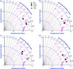
Taylor diagrams representations of all methods in the testing data. (a) raw, (b) SG: Savitzky-Golay, (c) SNV: standard normal variate, (d) MSC:
multiplicative scatter correction.

Figure 10
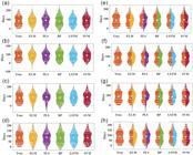
Violin-plot representations of all methods in the testing data. (a) raw, (e) raw compared, (b) Savitzky-Golay (SG), (f) Savitzky-Golay (SG) compared, (c) standard normal variate (SNV), (g) standard normal variate (SNV) compared, (d) multiplicative scatter correction (MSC), (h) multiplicative scatter correction (MSC) compared.

The Taylor diagrams of true and predicted value in Figure 9 provide a comprehensive visualization of model performance by simultaneously displaying three key statistical metrics: the correlation coefficient (R) between predicted and observed values (indicated by the azimuthal angle), the standard deviation (SD) of the predictions (indicated by the radial distance from the origin), and the centered root-mean-square difference (RMSD) (indicated by the distance from the reference point). The correlation coefficient measures the strength of the linear relationship between predicted and observed values, while the standard deviation indicates whether the model reproduces the variability of the observations. We expect the correlation coefficient to be as close to 1 as possible and the RMSD to be as close to 0 as possible. SVM coupled with MSC preprocessing achieved the highest correlation (R = 0.99), the most favorable standard deviation (SD = 7.23), and the lowest RMSD. This configuration represents the optimal balance across all three metrics. LSTM (R = 0.97, SD = 12.86) and BP (R = 0.96, SD = 15.56) form an intermediate cluster, exhibiting good correlation but moderate deviations in SD and RMSD. ELM and PLS showed the weakest performance, with lower correlation and substantially higher SD (> 20), indicating their limited suitability for stamp age prediction. Consequently, MSC-SVM can be adopted as the primary modeling approach for stamp age determination, while LSTM and BP offer acceptable alternatives with good correlation, albeit requiring careful consideration of their higher variability and RMSD.

Violin plots combine the summary statistics of box plots with the continuous probability density estimation of kernel density functions, providing an intuitive visualization of the central tendency, dispersion, and probability density of data distributions. Figure 10 presents violin plots illustrating the distributional characteristics of observed and predicted values under different configurations. In Figures 10a-10d, each violin represents the full distribution of either observed or predicted values under a specific configuration. Figures 10e-10h adopt a comparative structure: the left half of each violin displays the distribution of observed values, while the right half shows the distribution of predictions from different models, facilitating direct visual comparison of distributional alignment. In Figure 10h, the right half of the violin SVM (predictions) closely mirrors the shape and position of the left half (observations), indicating near-identical distributional characteristics. SVM captures the full range of observed values without significant truncation or extension, demonstrating appropriate handling of extreme cases. These findings corroborate the results from the Taylor diagram and cross-validation analyses, reinforcing the recommendation of MSC-SVM as the primary modeling approach for forensic stamp age determination, owing to its exceptional ability to reproduce the complete statistical distribution of stamp aging data.

This study demonstrates that the combination of MSC preprocessing and SVM regression is the most effective approach for addressing spectral prediction tasks of this nature. Freshly applied stamp ink contains volatile organic solvents that facilitate ink transfer and initial wetting. As these solvents evaporate over time, the physical matrix of the ink film undergoes densification, altering light scattering properties and refractive index. This process affects the baseline and slope of the entire reflectance spectrum, particularly in the near-infrared region where scattering dominates. MSC preprocessing, which specifically corrects multiplicative scattering effects, enhances the ability of the model to isolate these chemometric signals from physical artifacts. Additionally, different chemical components age at varying rates, creating a complex, multi-temporal spectral evolution pattern. The ability of SVM to integrate information across the full spectral range enables it to appropriately weight these temporally distinct signals, explaining its superior performance over linear methods such as PLS, which cannot capture such nonlinear, multi-process dynamics. This combination achieved the highest prediction accuracy while maintaining excellent generalization capability, effectively avoiding overfitting. The metric proved to be a concise and effective diagnostic tool, successfully identifying models such as SG-SVM and SNV-BP, which exhibited high training performance but were at risk of poor generalization. In model selection, priority should be given to models with outstanding test set performance and low values to achieve a balance between accuracy and robustness.

Limitations and future work

Although this study demonstrates the promising potential of combining hyperspectral imaging with machine learning for non-destructive stamp age determination, several limitations should be acknowledged, and corresponding future research directions are proposed accordingly: (i) the stamp samples were collected under controlled laboratory conditions with limited brand varieties and paper types. In real-world forensic scenarios, stamp impressions are exposed to diverse environmental factors (e.g., temperature, humidity, light exposure) and may appear on various paper substrates with different physicochemical properties. These factors could significantly influence the aging process of stamp inks and, consequently, the spectral signatures captured by hyperspectral imaging. Future research should expand the dataset to include a wider range of ink formulations, paper types, and storage conditions to enhance model generalizability and robustness in practical applications; (ii) although 10-fold cross-validation was employed to mitigate overfitting, the number of independent stamp impressions remains relatively limited. Multiple regions of interest (ROIs) extracted from the same stamp impression may introduce spatial autocorrelation and reduce sample independence, potentially leading to overly optimistic performance estimates. Future studies should collect a larger number of independent stamp samples to enable more rigorous validation, including external testing on completely independent datasets; (iii) the aging experiments were conducted under controlled laboratory conditions, which may not fully replicate the complex and variable environments encountered in real forensic casework. Factors such as fluctuations in temperature and humidity, exposure to different light sources, and potential contamination could alter the aging trajectory and spectral response of stamp inks. Future investigations should include accelerated aging studies under controlled environmental chambers and, where possible, validation on naturally aged casework samples to assess model performance under realistic conditions.

Conclusions

This study successfully developed a prediction model for the aging time of stamp impressions created with oil-based inks, based on hyperspectral imaging technology combined with a SVM algorithm. By collecting hyperspectral data of different brand stamp inks at different time points and applying preprocessing techniques MSC, the signal to noise ratio and feature separability of the spectral data were significantly enhanced. The SVM model demonstrated optimal performance on the test set, notably surpassing LSTM, PLS, BP, and ELM models. The results indicate that hyperspectral imaging technology can effectively capture the chemical changes in ink composition over time (such as volatilization, oxidation, and carrier medium migration), while the SVM algorithm, through nonlinear kernel functions, achieved high-accuracy modeling of the time-spectral relationship. This provides a reliable technical approach for the non-destructive and rapid determination of stamp impression age. Nevertheless, the study still faces certain technical limitations, including insufficient sample diversity, limited temporal coverage, and a lack of controlled environmental factors. Future work should expand the variety of ink and paper types, extend the observation period, incorporate environmental variable modeling, and integrate deep learning techniques along with the development of portable devices to enhance generalizability and practicality. Additionally, coupling chromatographic mass spectrometric analyses could further elucidate the aging mechanisms, thereby strengthening the theoretical foundation of the model.

Data Availability Statement

The research data should be requested from the corresponding author.

Acknowledgments

The authors gratefully acknowledge the financial support provided by Research Fund Project of Yunnan Provincial Department of Education (grant No. 2026J0799), Key Project of Yunnan Police College (grant No. 19A019). Yunnan Police College Research Project (202523001034ZR-003).

References

• ¹ Lee, J.; Lee, C.; Lee, K.; Appl. Surf. Sci. 2008, 255, 1523. [Crossref]
  » Crossref
• ² Cieśla, R.; Int. J. Conserv. Sci. 2023, 2, 481. [Crossref]
  » Crossref
• ³ Canh, T. T.; Sch. Int. J. Law Crime Justice 2025, 8, 261. [Crossref]
  » Crossref
• ⁴ Goc, M.; Miron, M.; Probl. Krym. 2014, 284, 17. [Crossref]
  » Crossref
• ⁵ Li, B.; J. Forensic Sci. 2014, 59, 1403. [Crossref]
  » Crossref
• ⁶ Yao, Y.-T.; Song, J.; Yu, J.; Wang, X.-F.; Hou, F.; Zhang, A.L.; Liu, Y.; Han, J.; Xie, M.-X.; J. Sep. Sci. 2009, 32, 2919. [Crossref]
  » Crossref
• ⁷ Grechukha, N. M.; Gorshkova, K. O.; Panov, M. S.; Tumkin, I. I.; Kirillova, E. O.; Lukianov, V. V.; Kochemirovsky, V. A.; Appl. Sci. 2017, 7, 991. [Crossref]
  » Crossref
• ⁸ Islek, D. S.; Isat, E.; Cengiz, S.; Med. Sci 2018, 7, 166. [Crossref]
  » Crossref
• ⁹ Islek, D. S.; NOFOR 2023, 2, 9. [Crossref]
  » Crossref
• ¹⁰ Li, B.; J. Forensic Sci. 2014, 59, 1403. [Crossref]
  » Crossref
• ¹¹ Bügler, J. H.; Buchner, H.; Dallmayer, A.; J. Forensic Sci. 2008, 53, 982. [Crossref]
  » Crossref
• ¹² Khan, Z.; Faisal, S.; Ajmal, M.; Pattern Recognit 2015, 48, 3615. [Crossref]
  » Crossref
• ¹³ Sun, D. W.; Pu, H.; Yu, J.; Nat. Rev. Electr. Eng. 2024, 1, 251. [Crossref]
  » Crossref
• ¹⁴ Wang, B.; Sun, J.; Xia, L.; Liu, J.; Wang, Z.; Li, P.; Sun, X.; Food Rev. Int 2023, 39, 1043. [Crossref]
  » Crossref
• ¹⁵ Babini, A.; Frascella, S.; Sech, G.; Andriulo, F.; Cannella, F.; Marchello, G.; Traviglia, A.; Heritage 2025, 8, 417. [Crossref]
  » Crossref
• ¹⁶ Pradeep, A. S.; Babu, J.; Sandana, J. S.; Deivalakshmi, S.; Forensic Sci. Int 2024, 364, 112. [Crossref]
  » Crossref
• ¹⁷ Babu, A. S.; Tomar, A.; Sharma, S.; Crit. Rev. Anal. Chem. 2025, 55, 292. [Crossref]
  » Crossref
• ¹⁸ Lu, X.; Zhang, J.; Li, F.; Wu, J.; Zhang, X.; Ren, H.; Ma, K.; Anal. Methods 2025, 17, 7519. [Crossref]
  » Crossref
• ¹⁹ Lu, X.; Zhang, J.; Wu, J.; Zhang, X.; Ren, H.; Chen, H.; Li, F.; Anal. Methods 2025, 17, 7722. [Crossref]
  » Crossref
• ²⁰ Mair, C.; Kadoda, G.; Lefley, M.; Phalp, K.; Schofield, C.; Shepperd, M.; Webster, S.; J. Syst. Software 2000, 5, 23. [Crossref]
  » Crossref
• ²¹ Liang, Y.; Wu, J.; Zeng, Q.; Zhao, Y.; Ma, K.; Zhang, X.; Qi, Y.; J. Braz. Chem. Soc. 2024, 35, 23. [Crossref]
  » Crossref
• ²² Haut, J. M.; Franco-Valiente, J. M.; Paoletti, M. E.; SN Comput. Sci. 2024, 5, 719. [Crossref]
  » Crossref
• ²³ Yang, H.; Qu, F.; Yang, Y.; Sensors 2024, 24, 4635. [Crossref]
  » Crossref
• ²⁴ LeCun, Y.; Bengio, Y.; Hinton, G.; Nature 2015, 521, 436. [Crossref]
  » Crossref
• ²⁵ Huang, G. B.; Zhu, Q. Y.; Siew, C. K.; Neurocomputing 2006, 70, 489. [Crossref]
  » Crossref
• ²⁶ Mao, B.; Cheng, Q.; Chen, L.; Comput. Electron. Agric. 2024, 222, 109046. [Crossref]
  » Crossref
• ²⁷ Citakoglu, H.; Arabian J. Geosci. 2021, 14, 2131. [Crossref]
  » Crossref
• ²⁸ Samadianfard, S.; Rousta, Z.; Mohebbiyan, M.; Talebi, H.; Earth Sci. Inform. 2025, 18, 448. [Crossref]
  » Crossref
• ²⁹ Bian, L.; Wang, Z.; Zhang, Y.; Nature 2024, 635, 73. [Crossref]
  » Crossref
• ³⁰ Landgrebe, D.; IEEE Signal Process. Mag. 2002, 191, 17. [Crossref]
  » Crossref
• ³¹ ElMasry, G.; Sun, D.-W. In Hyperspectral Imaging for Food Quality Analysis and Control; Sun, D.-W., ed.; Academic Press: London, UK, 2010. [Crossref]
  » Crossref
• ³² Hearst, M. A.; Dumais, S. T.; Osuna, E.; Platt, J.; Scholkopf, B.; IEEE Intell. Syst. Their Appl. 1998, 13, 18. [Crossref]
  » Crossref
• ³³ Yalçın, G.; Bayram, S.; Çıtakoğlu, H.; Buildings 2024, 14, 3772. [Crossref]
  » Crossref
• ³⁴ Simsek, O.; Citakoglu, H.; Gumus, V.; Pure Appl. Geophys. 2025, 182, 3107. [Crossref]
  » Crossref
• ³⁵ Nash, J. E.; Sutcliffe, J.V.; J. Hydrol 1970, 10, 282. [Crossref]
  » Crossref
• ³⁶ Acar, E. F.; Sun, L.; Biometrics 2013, 69, 427. [Crossref]
  » Crossref

Edited by

• Editor handled this article:
  Paula Homem-de-Mello (Executive)

Publication Dates

• Publication in this collection
  06 July 2026
• Date of issue
  2026

History

• Received
  26 Dec 2025
• Accepted
  19 May 2026