Evaluation of Different Normalization Strategies for Metabolomics Data Acquired by Gas Chromatography-Mass Spectrometry

Abstract

Untargeted metabolomics data are highly complex and variable. One of the major challenges in processing them is ensuring that biological interpretations reflect the organism metabolic variability rather than undesirable factors arising from random or systematic experimental errors. Here, nine post-acquisition normalization strategies were evaluated on two gas chromatography-mass spectrometry (GC-MS) metabolomics datasets (cellular and serum). GC-MS data are particularly affected by experimental variability since derivatization steps are required. Thus, the use of internal standards (IS) is indicated, although not mandatory. When an IS is not available, post-acquisition normalization methods help correct for variations. Mean, median, and EigenMS normalization proved quite suitable for both datasets, as evidenced by good sample and quality control grouping and within-group relative log abundance (RLA). EigenMS was chosen due to its improved sample grouping. Strategies that use a sample as a reference factor for normalization did not demonstrate the same efficiency, as they introduced biases into the multivariate models. This could be due to a poor choice of reference sample, which compromises the fit of the data matrix. The results observed in this study demonstrate the importance of testing different normalization methods in any metabolomics study to help obtain more robust and reliable matrices for data inspection and interpretation.

Keywords:
Trypanosoma cruzi; feline mammary carcinoma; global metabolomics; data processing; data normalization; biological variability

Introduction

Untargeted metabolomics is an approach that enables the understanding of metabolic changes at the molecular level by analyzing as many metabolites as possible in biological organisms. This is a constantly growing field that is being applied to the discovery of biomarkers, the development of new therapies, and diagnostic and prognostic purposes, as well as toxicological and environmental analyses.¹,² The experiments are conducted comparatively, using various biological samples, including blood (serum or plasma), urine, saliva, tissues, cells, sugar, and hair, among others.

Biological samples are non-homogeneous specimens, in which variations in size, weight, and volume cause significant changes in the concentrations of metabolites after extraction.³ Analytical factors, such as differences in derivatization efficiency, storage conditions, and instrumental variations, also contribute to increased variability in detected metabolite levels. Normalization strategies are then used to minimize and remove random and systematic variations in measurements, allowing biological interpretations to be associated with the studied condition and not with errors in experimental design, sample preparation, or data acquisition.⁴

A wide variety of normalization methods are found in metabolomics studies, which can be divided into three strategies: chemical, statistical, and sample-based normalization. Chemical normalization consists of normalization by detecting an added internal standard (IS). However, considering untargeted studies, choosing an IS can be challenging. The high cost of isotopically labeled standards and the need to add multiple standards to account for corrections during sample preparation make their use impractical.⁴,⁵ Statistical normalization includes post-acquisition strategies such as correction by sum, median, mean, likelihood ratio, quantile, total area, and quality control (QC) samples, among others. These strategies are effective at reducing systematic variation. However, some of these normalization methods can introduce artificial correlations into the data, requiring caution in their application.⁴,⁶ Sample-based normalization is applied in specific cases due to sample characteristics. For example, solid samples should be normalized to biomass or dry mass, whereas urine samples, which vary in dilution and consequently in metabolite concentration, are commonly normalized to creatinine content and osmolality.

Some studies have focused on evaluating different normalization strategies for untargeted metabolomics data, primarily in cell samples and urine using liquid chromatography-mass spectrometry (LC-MS).⁶-⁹ Urine samples exhibit significant variability in metabolite concentrations, influenced by factors such as water intake, eating habits, and diet. Cell samples exhibit low within-group metabolic variability; however, variations in water content, cell number, and density significantly affect metabolite concentrations.¹⁰,¹¹ Blood samples (plasma and serum) and tissues are considered homeostatically regulated. Therefore, the high variability observed in such samples is associated with biological disorders.¹⁰,¹²,¹³

Specifically, data acquired by gas chromatography-mass spectrometry (GC-MS) are susceptible to unwanted variation due to errors and inefficiencies in the chemical derivatization steps, requiring normalization. Some researchers have been making efforts to find the best normalization strategy for different datasets acquired by GC-MS, including dog food,¹⁰ zebrafish,¹⁴ adherent cells,¹⁵,¹⁶ urine,¹⁷,¹⁸ and serum samples.¹⁸-²⁰ Normalization strategies are tested according to software availability and suitability for each study. Overall, the studies demonstrate the absence of a gold-standard normalization method. Combining two or more strategies to reduce artificial correlations arising from sample type and preparation steps enables more accurate biological interpretation.

Thus, given the importance of the normalization step in metabolomics studies, this work systematically evaluated nine normalization strategies across two sample sets: Trypanosoma cruzi cell samples and blood serum samples from female cats with mammary cancer.

Methodology

Data sets

Two untargeted metabolomics datasets acquired by GC-MS, previously studied by our group, were used in this work:²¹

(i) Cell dataset: this data was from a study evaluating the metabolic changes resulting from the interaction of Trypanosoma cruzi parasites with the extracellular matrix. The data of 16 samples, divided into two groups (control, n = 5, and test, n = 5) and quality controls (QC, n = 6);

(ii) Serum dataset: this data was from a study to understand feline mammary carcinoma, and the results were recently submitted for publication. Serum samples from female cats (n = 36) comprising two groups (cancer, n = 17, and control, n = 10), and QC (n = 9).

GC-MS equipment²¹

Cell dataset was acquired in a GC-MS system (GC 7890A and MS 5975C inert XL, Agilent Technologies, CA, USA) and serum dataset were acquired in a GC-MS equipment (GCMS-QP2010 Ultra, Shimadzu, Kyoto, Japan). The methods were adapted to the equipment. Briefly, metabolite separation was performed in a DB 5MS column (30 m length × 0.25 mm i.d., 0.25 mm film composed of 95% dimethyl / 5% diphenyl polysiloxane, Agilent Technologies). Helium was the carrier gas at 1.0 mL min^-1. A volume of 1 µL of the samples was injected with 1:10 split and the injector was kept at 250 ºC. Initial oven temperature was set at 60 ºC and hold for 1 min, followed by 10 ºC min^-1 ramp up to 300 ºC. Transfer line, filament source, and quadrupole temperatures were maintained at 290, 230 and 150 ºC, respectively. The MS was operated in scan mode (50-600 m/z) and electron impact ionization (70 eV).²¹

Data processing

The raw data files were converted to .abf format using Reiyfics ABF converter 4.0 software (Reifycs Inc., Japan). Raw data matrices were extracted in MS-DIAL 5.3 (RIKEN, Japan and UC Davis, USA) using hard ionization (GC-MS) and centroid data. The data collection was carried out with a mass range of 50-600 m/z for cells and 40-600 m/z for serum, and an t_R range of 6-25 and 5-30 min for cells and serum, respectively. Peak detection was performed with a minimum peak height of 300 counts for cells and 10000 counts for serum; mass slice width and mass accuracy for centroid were set to 0.5 m/z for both data sets. The smoothing method applied was linear weight moving average with a smoothing level of 1 for cells and 2 for serum, and an average peak width of 10 scans for both datasets. For spectrum deconvolution, a sigma window value of 0.5 and an electron ionization (EI) spectral cutoff of 1 unit for the cell dataset and 10 units for the serum dataset were used.

Metabolite annotation was performed using three MSP spectra databases: FiehnLIB and Kasuza, and the Human Metabolome Database (HMDB), using a score greater than 85 from the comparison of library spectra with the samples. Metabolites with a maximum intensity (sample)/blank intensity ratio greater than five were excluded from the extracted raw data table. The NOREVA 2.0 software²² (Zhejiang University and Chongqing University, China) was used to filter the data using a 30% relative standard deviation (RSD) cutoff for the QC samples, and to impute using the k-nearest neighbors (KNN) algorithm, which corrects the QCs based on a local polynomial regression and a logarithmic transformation. In the final step, the quality control robust LOESS signal correction (QC-RLSC, LOESS: local polynomial regression fitting) was performed to adjust time-dependent instrumental deviations. Local polynomial fits were selected as a regression model for QC samples correction.

Normalization methods

Nine post-acquisition normalization strategies were tested and compared across the two datasets: contrast, EigenMS, linear baseline, mass spectrometry total useful signal (MSTUS), mean, median, probabilistic quotient normalization (PQN), quantile, and total sum:

(i) Contrast: it is a non-linear method that transforms the data into a new basis (the contrasts), fits a smooth curve (by LOESS) to eliminate systematic differences and ensure that the characteristics retain the same values after normalization, and returns to the original scale, normalizing the data;²³

(ii) EigenMS: this method identifies and removes systematic bias from the data, preserving biological differences between groups. It filters out technical noise arising from differences in signal intensity between MS and is well-suited for handling missing values;²⁴

(iii) Linear baseline: it uses a sample as a reference and adjusts the other samples by a linear constant factor, whereby all samples remain on the same scale. The result depends on the reference sample, and this method has the limitation of not correcting for non-linear relationships;²⁵

(iv) Mass spectrometry total useful signal (MSTUS): initially applied for normalization of LC-MS data in urine samples, MSTUS uses the useful signals, common peaks, from all samples under study, dividing each intensity by the sum of the useful signals;²⁶

(v) Mean: the data are normalized by the average value of their intensities (reference), therefore being suitable for data that follow a normal distribution. Since it uses all available information from the data, it is subject to outlier effects if they are not properly removed;⁸,²⁷

(vi) Median: it is performed based on the median intensity of the metabolites. It is similar to MSTUS; however, the influence of the most intense metabolites is reduced, assuming they remain constant across samples. Median normalization adjusts the data using a central value to reduce outlier effects, while MSTUS corrects spectra based on the total useful signal of the sample;¹⁸

(vii) PQN: this method is based on calculating a normalization factor for each feature as a function of the average response among the QC samples or a reference sample. The specific normalization factor is used to divide and adjust the intensities of each sample;²⁸

(viii) Quantile: this normalization restructures the data so that all samples share the same distribution. The process consists of ranking the intensities of each sample (from lowest to highest), generating a reference mean distribution based on these ranks, and finally replacing the original data with reference values, preserving the identity of each metabolite;²⁹

(ix) Total sum: this method consists of calculating a normalization factor for each sample, corresponding to the total sum of abundances or the sum of the squares of intensities, and dividing each metabolite by this value. This procedure ensures that all samples have the same final sum (or vector norm), correcting concentration discrepancies.³⁰

In the serum dataset, an internal standard (IS) C13 methyl ester (10 mg mL^-1) was added to the derivatized extracts. The IS peak intensity was then used as a normalization strategy (pre-acquisition normalization), evaluated as a single normalization method, and associated with the other nine strategies tested. Normalization was performed in the NOREVA 2.0 software.²²

Statistical analysis

The normalized data were logarithmically transformed and Pareto-scaled before statistical analysis to reduce the influence of a wide concentration range of extracted m/z values resulting from variations in derivatization subproducts and generated fragments in the ion source. Multivariate analyses were performed in the MetaboAnalyst 6.0 platform (University of Alberta and National Institute for Nanotechnology, Canada),³¹ applying principal component analysis (PCA) to evaluate data normalization by clustering QCs and sample groups, and orthogonal partial least squares-discriminant analysis (OPLS-DA) to identify metabolites responsible for separating the sample groups. Permutation tests (n = 1000) were applied to the supervised OPLS-DA models, and significant metabolites were determined based on variable importance on projection analysis (VIP score > 1.0).

Results and Discussion

In this work, two datasets (cells and serum) from untargeted metabolomics studies were used to investigate the impact of different normalization strategies on the results. The chosen datasets exhibit different characteristics with respect to the sample matrix and are subject to distinct biological variations. Blood serum is a relatively homogeneous biological matrix compared to other biofluids, such as urine and feces, leading to minimal variation. However, blood fluids provide a less specific response, since metabolic changes reflect the entire organism, being a matrix sensitive to environmental effects, diet, genetic variations, and diseases.³² Cellular samples correspond to more controlled organisms, since it is possible to standardize cell growth under the same conditions. However, it is difficult to control the quantity of cells collected, leading to variation in metabolite abundance between groups.¹³

The efficiency of a normalization method is measured by its ability to reduce variation within the same group, and PCA is among the best methods for this evaluation.¹³ Figures S1 and S2 (Supplementary Information (SI) section) present all score plots from unsupervised PCA models of cell and serum data, respectively. PCA analysis reduces data dimensionality, highlighting the relevant information in the investigated dataset. Thus, the analysis allowed us to compare the effect of the nine normalization strategies evaluated (contrast, EigenMS, linear baseline, MSTUS, mean, median, PQN, quantile, and total sum), as well as the grouping of data without applying normalization.

Specifically, for the serum dataset (Figure S2, in the SI section), an internal standard (IS) was used in data acquisition. Thus, IS normalization was applied both individually and associated with the nine strategies studied. Normalization with internal standards aims to reduce technical variations in sample preparation and instrumental analysis. The use of IS in metabolomics studies is encouraged; however, it is not always applied. Therefore, other normalization strategies can be used to help correct systematic and random variations. Mean, median, or total sum are strategies commonly used when an IS is unavailable.³³ However, these strategies have already demonstrated the introduction of biases, especially for data with large differences between sample groups.¹¹ Other important limitations involve the use of reference samples as a basis for normalization, as in the linear baseline and PQN methods.²⁷ In these cases, the normalized matrices may vary slightly depending on the chosen reference sample. This limitation is particularly evident in GC-MS data, due to variations in the intensities of the derivatization products. The variability in the data is associated with each study, due to the type of specimen under investigation, the experimental procedures, and the biological influence of the condition being studied.

Overall, the models presented in Figures S1 and S2, in the SI section) showed drastic differences in sample and QC groupings across the two datasets investigated. In both cases, normalizations using contrast, linear baseline, and MSTUS resulted in biased sample groupings, suggesting the presence of outliers (Figures S1 and S2, in the SI section). PQN-based normalization was also unsatisfactory for the cells dataset evaluation (Figure S1h, in the SI section). After a careful inspection of all raw data using total ion chromatograms, extracted feature tables, and heatmaps, no clear outliers were found, reinforcing the idea that these normalization strategies introduce biases in the data grouping. The loading plots, presented in Figures S3 and S4 (SI section) for cells and serum, respectively, corroborate the results. The analysis of the loadings showed clearly biased clustering profiles for contrast in cell samples (Figure S3b, in the SI section) and for contrast, linear baseline, and MSTUS in serum samples (Figures S4c, S4e, and S4h (SI section), respectively).

Table 1 presents the quality parameters of the PCA models, including explained variance, Fisher’s F-value, coefficient of determination (R²), and p-value. In the analysis of the cell dataset, contrast, EigenMS, mean, median, PQN, quantile, total serum, and non-normalized data were found to be statistically significant (p-value < 0.05). In the serum dataset analyses, seven normalization strategies were not significant (p-value > 0.05); only IS, EigenMS, quantile normalization, and the raw data matrix (without normalization) had p-values < 0.05.

Table 1
Statistical parameters of the unsupervised PCA model for evaluating different normalization strategies for two metabolomics datasets acquired by GC-MS

Normalization	Cell dataset					Serum dataset
	PC1 × PC2	F-value	R2	p-value		PC1 × PC2	F-value	R2	p-value
None	75.3	28.8	0.82	0.001		45.2	3.62	0.18	0.03
IS	-	-	-	-		44.1	3.55	0.18	0.01
Contrast	85.2	5.29	0.45	0.003		89.5	0.31	0.02	0.94
EigenMS	83.7	242	0.97	0.001		40.4	12.8	0.44	0.001
Linear baseline	97.9	0.84	0.11	0.740		70.9	1.76	0.09	0.06
Mean	82.6	34.6	0.84	0.001		28.8	1.92	0.10	0.12
Median	80.4	34.8	0.84	0.001		28.7	1.93	0.10	0.11
MSTUS	97.9	0.84	0.11	0.770		70.9	1.76	0.09	0.08
PQN	99.8	0.77	0.10	0.94		76.3	0.77	0.04	0.67
Quantile	72.4	13.6	0.68	0.001		29.8	6.87	0.29	0.001
Total-sum	100	84.2	0.93	0.001		100	4.30	0.21	0.03

Despite being significant, the models obtained for normalization with IS alone, and quantile did not show good QC and sample groupings (Figure S2, in the SI section), with unsatisfactory parameters for the unsupervised models (Table 1). The IS alone did not outperform EigenMS-based normalization. It was hypothesized that corrections after normalization to IS were minimal, since IS was added to the extracts after the derivatization procedure. Thus, experimental variations in this step of sample preparation could not be corrected. Furthermore, using a single IS is often insufficient to correct for all systematic errors, as the variations captured by an IS are inherently tied to its specific chemical properties and may not reflect the behavior of all metabolites.³⁰ Thus, ideally, more than one IS should be added before the extraction process or, at least, before derivatization to compensate for reaction inefficiencies. Some injection corrections may have occurred. However, losses due to volatilization of extracts that remained longer in the sampler until analysis may have impaired the reproducibility of IS in the samples, as evidenced by the dispersion of the QCs (Figure S1).

Non-normalized models are also presented in Figures S1 to S4 (SI section) and, together with the parameters in Table 1, suggest that no normalization is necessary for these datasets. However, this is not a valid conclusion, especially given the enormous variability in biological data and analytical variations. This (non-biological) variability can lead to erroneous biological interpretations of the studies. The multiple steps involved in the metabolomics workflow, ranging from sampling, sample preparation, and data acquisition, are the main contributors to the introduction of variability. For GC-MS data, a derivatization step is required to make the metabolites volatile and thermally stable. The process itself introduces errors arising from incomplete derivatization, evaporation losses, and poor dissolution of some metabolites.

Additionally, the derivatization is performed individually for each sample, reducing the reproducibility of the QC samples. Finally, the loss of metabolites due to degradation and evaporation during long analytical sequences increases variability in the system.³⁴,³⁵ Thus, the normalization step is fundamental for analyzing data acquired by GC-MS.

The impact of normalization strategies on data transformation and dispersion can also be assessed using within-group relative log abundance (RLA) plots, presented in Figures S5 and S6 (SI section). Within-group RLA plots are generated after calculating the median of each metabolite within each experimental group (factor of interest), followed by subtracting this value from the original intensity of each corresponding sample. The results are visualized by boxplots of this centered data matrix. A good normalization method should produce homogeneous distributions of boxplots within each group, with medians close to zero, indicating the removal of undesirable technical variation within the groups.³⁰ Within-group RLA plots demonstrate how the data were adjusted after applying each normalization method and allow us to verify the overall impact on the datasets. As expected, the data distribution before normalization highlights the need to apply adjustment strategies before multivariate statistical analyses. The results presented in Figures S5 and S6 (SI section) indicate that contrast, linear baseline, MSTUS, PQN, and total sum normalization strategies showed the greatest dispersion, while EigenMS, mean, median, and quantile showed the least.

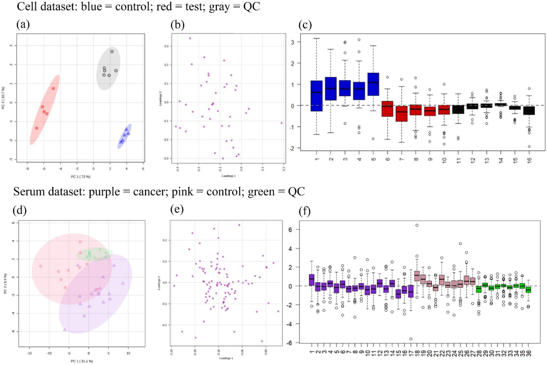
EigenMS, mean, median, and quantile demonstrated the best groupings and appropriate parameters for the PCA models (R² > 0.67, F > 13.5, and p-value = 0.001; Figure S1) for the cell dataset and could be used to normalize these data. However, the samples and QCs were more clustered with EigenMS normalization (Figure S1c, SI section), as reflected in the model quality and statistical parameters, which showed the best values: F = 242.48, R² = 0.97, and p-value = 0.001 (Table 1). For the serum dataset, greater data dispersion is observed (Figure S2) due to the greater natural variability among the samples, since each sample corresponds to a different animal with different habits and diets. In this sample set, EigenMS also yielded the best statistical parameters (F = 12.8 and p-value = 0.001; Figure S2d and Table 1) and better QC grouping. It is interesting to note that the models with the highest explained variances (Table 1) are not always the most suitable, as evidenced by the linear baseline, PQN, and MSTUS strategies in both datasets. In these cases, a careful analysis of the dispersion of variables by RLA and loadings is essential to determine whether data bias is present.

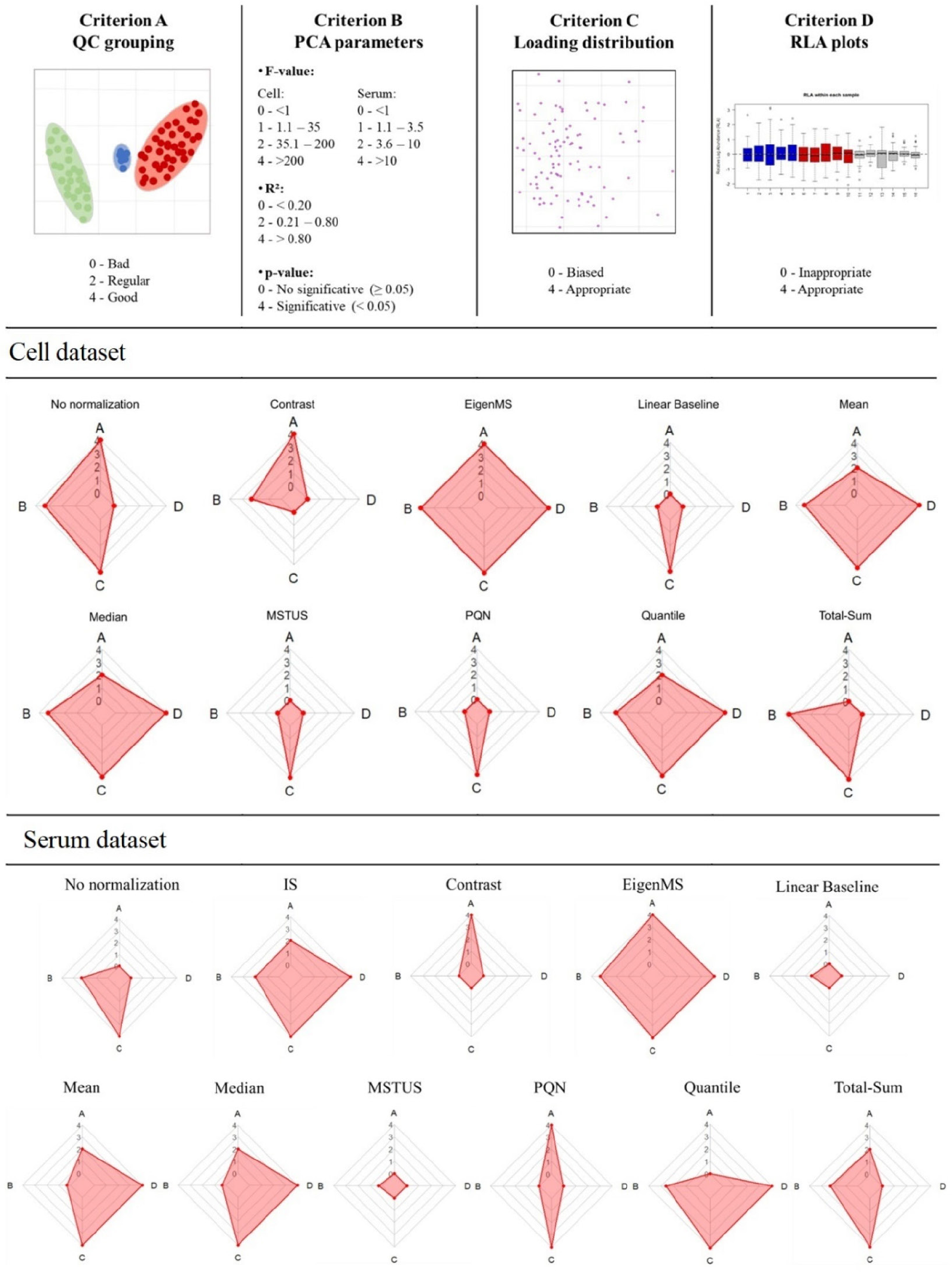
The performance of the evaluated normalization strategies could finally be assessed by analyzing four complementary criteria: (A) QC grouping; (B) PCA parameters; (C) loading plots; and (D) RLA plots. Figure 1 presents the metrics used in each criterion and the results presented as radar plots, facilitating a direct visual comparison of the methods across both cell and serum datasets. The variables distribution, evaluated by loadings and RLA plots, followed by QC grouping, were the most important metrics. The quality of the unsupervised models was evaluated as an average of the significance (p and F values), with significant models having greater weight in the metric, and by the coefficient of determination (R²). This collective criterion helps improve the understanding of result evaluation. Thus, across both datasets, normalization by EigenMS best met the evaluated criteria and was selected for application in subsequent processing steps.

Figure 1
Performance assessment of the normalization strategies for cell and serum dataset based on four criteria - criterion A: QC grouping in PCA model; criterion B: statistical parameters of PCA model; criterion C: loading plots; and criterion D: within-group relative log abundance (RLA) plots.

EigenMS is a normalization method based on singular value decomposition, identifies and removes undesirable systematic variations in the data, preserves biological variability,²⁴ and has proven helpful for metabolomics data. Figure 2 presents the multivariate models, loadings, and within-group relative log abundance using the EigenMS strategy in our investigated datasets. An inspection of the PCAs and parameters in Table 1 shows that two principal components presented 83.7 and 40.4% of the explained variance in the cell and serum datasets, respectively.

Figure 2
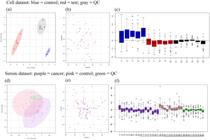
EigenMS normalization results applied to cellular (up) and serum (down) GC-MS datasets; (a) and (d) unsupervised PCA score plots; (b) and (e) loading plots; (c) and (f) within-group RLA plots.

Normalization was not the only correction factor applied to the datasets. Missing values imputation using k-nearest neighbors was also performed on the NOREVA platform.²² KNN is considered one of the most robust methods for imputing metabolomic data because it finds k-value metabolites of interest that are similar to those with missing values.²⁹ The KNN method has already been shown to be a suitable imputation strategy for untargeted metabolomics data.⁶ The application of different data imputation strategies should be carried out with caution, especially in datasets with a large number of missing values. Such strategies can introduce artificial data, leading to incorrect interpretation of the results. In this work, the proportion of missing values decreased from 24.7 to 2.35% in the cell dataset and from 5.76 to 0.25% in the serum dataset.

Finally, QC-RLSC was applied to remove instrumental deviations associated with the time sequence of data acquisition. The QC-RLSC method uses QC samples evaluated throughout the analytical sequence.²⁹,³⁶ This strategy is particularly interesting for GC-MS data, since the samples have been subjected to derivatization reactions whose efficiency varies randomly. Moreover, the samples are subject to losses due to the long waiting times of the analytical sequence.

Once the best normalization strategy was defined, data scaling methods were also evaluated. Scaling of metabolomic data is necessary because metabolites vary widely in concentration across study groups, and multivariate models aim to maximize data variance. Therefore, metabolites at higher levels could mask less abundant ones, hindering biological interpretation.²⁹

Auto, Pareto, interval, and level scaling were evaluated in MetaboAnalyst (Figures S7 and S8, in SI section). For the cellular dataset, the PCA models showed the same quality parameters (R² and explained variance), statistical significance (p-value < 0.05), and a good sample grouping. However, when evaluating the loading plots, it becomes clear that level and auto scaling introduce biases into the data (Figure S7, in SI section). Pareto and range scaling showed the best QC grouping and the greatest dispersion of loadings, preserving the variables distribution without introducing bias. Nevertheless, Pareto scaling showed slightly better QC grouping than range scaling and greater significance (F-value 242).

For the serum dataset (Figure S8, in SI section), level scaling, despite a higher R² and F-value, drastically influenced variables dispersion, as observed in the loadings plot. The other scaling methods (Figure S8, in SI section) showed similar results in terms of explained variance and significant p-value. Pareto scaling, however, also showed better performance for the serum dataset, with an R² of 0.44, a higher F-value, and better QC grouping. Therefore, Pareto scaling was chosen for application in both datasets. In Pareto scaling, each variable is centered on its mean, and the result is divided by the square root of standard deviation of each variable.³³

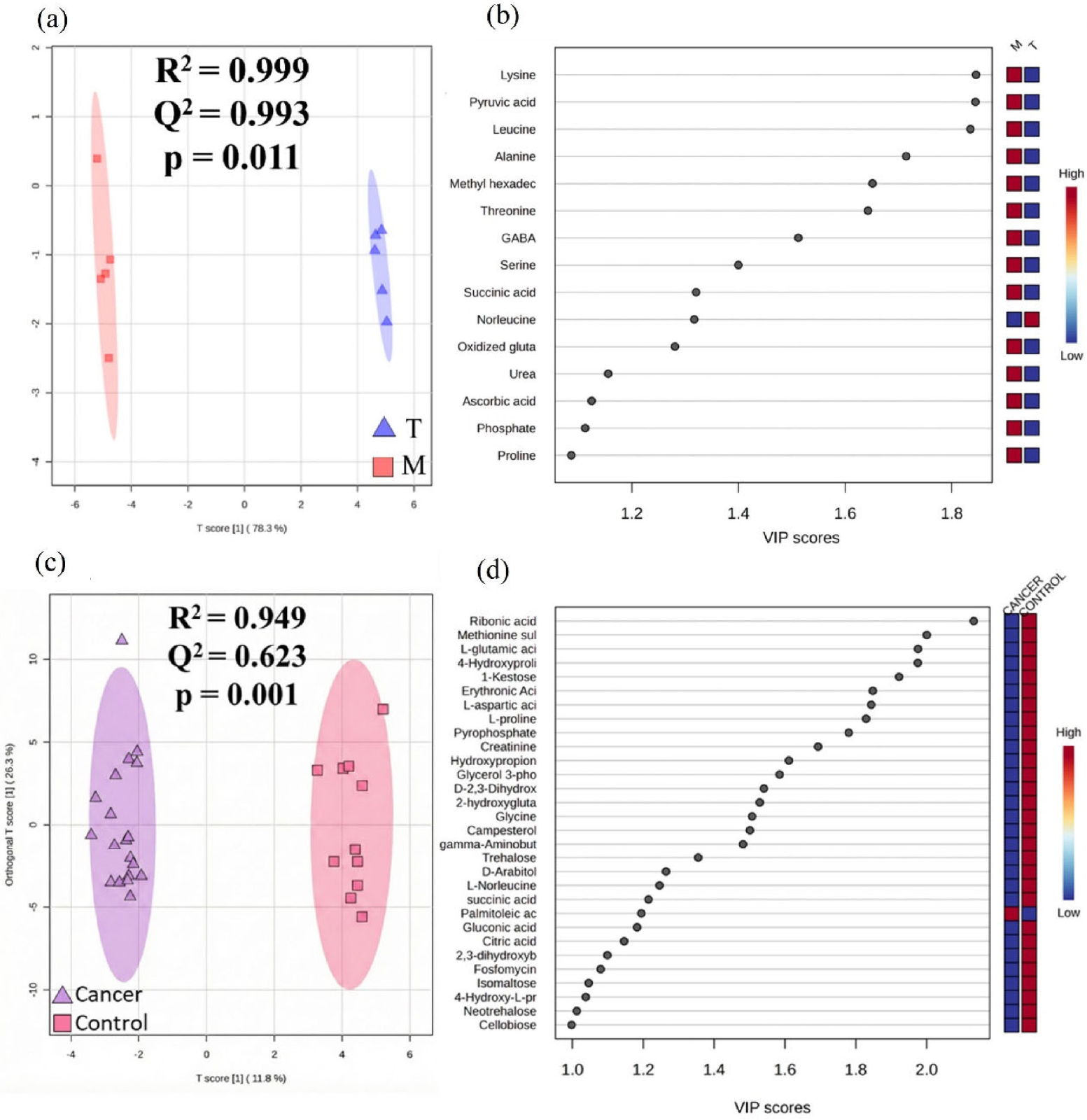
After determining the best strategies for normalization, transformation, and scaling of the datasets, supervised multivariate analyses are performed to maximize group differences and identify significant metabolites. OPLS-DA analyses were carried out. The models showed excellent quality parameters: goodness-of-fit (R²) > 0.99 for both studies, and predictive capabilities (Q²) of 0.993 for cell and 0.623 for serum. This supervised method should be used with caution, as it is prone to overfitting, especially in studies with many variables and a small sample size. Therefore, it is necessary to check whether the model is correctly adjusting the variables during group separation, and not just the noise. Thus, cross-validation must be performed to ensure proper performance of the model. In our study, the models were duly validated using permutation tests (n = 1000), yielding p-values < 0.01. In addition to the supervised model, the analyst must be aware of the unsupervised model (PCA), which indicates whether the groups under investigation are separated.

Finally, the discriminating metabolites were determined using VIP analysis (VIP > 1.0), yielding 15 and 30 significant metabolites in the analyses of T. cruzi cells and feline mammary cancer, respectively. It is important to note that none of the significant metabolites presented missing values, as these had been previously corrected using the KNN imputation method. Figure 3 presents the results of the OPLS-DA analysis, which were performance was evaluated using the AUC (area under the curve) metric.

Figure 3
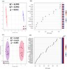
Supervised multivariate analysis with best condition of data normalization in cell and serum datasets: (a) OPLS-DA scores plot of cell dataset (R² = 0.999 and Q² = 0.993), (b) VIP scores plot of cell dataset, (c) OPLS-DA scores plot of serum dataset (R² = 0.949 and Q² = 0.623), and (d) VIP scores plot of serum dataset.

AUC is calculated from the significant information of the OPLS-DA using the ROC (receiver operating characteristic) curve. An AUC of 1.0 (95% confidence interval: 1.0-1.0) was obtained for the cell dataset, while the serum dataset yielded an AUC of 0.944 (95% confidence interval: 0.806-1.0). AUC values range from 0.5 to 1.0; the closer to the unit, the better the ability of the model to distinguish the groups under analysis. It is important to emphasize that supervised analyses were not used to determine the best data normalization, transformation, or scaling strategies. These assessments are merely supportive and help to verify that the normalization strategies applied were effective in constructing robust models, enabling future evaluation of biological effects in each study. However, these interpretations are outside the scope of this work.

Although the results presented here indicate that EigenMS is the best normalization strategy, it is important to note that the intrinsic variability of samples across different metabolomic datasets, combined with the analytical variations of the process, affects each study differently. Factors such as convenience, cost (when using internal standards), processing speed, ease of use, and availability of normalization platforms should also be considered. Therefore, a systematic evaluation of different normalization methods is strongly recommended in metabolomic studies.

Conclusions

In a metabolomics study, variations in metabolite levels are related to the specimen under investigation, sample preparation, and data acquisition, and, naturally, to the intrinsic biological variability of the samples. The best strategy to minimize systematic and random errors in the experimental process is to apply normalization methods. Evaluating different normalization strategies is a fundamental step in metabolomics data processing. This work presents an evaluation of normalization strategies in two completely different datasets. The first dataset involved more controlled sampling (cell samples), while the other (serum samples) had greater variability due to samples from different individuals with different habits. For both datasets, normalization using EigenMS improved sample grouping and quality control, enhanced variable dispersion, and resulted in high-quality cross-validated multivariate models. Although the result is consistent, it cannot be generalized to any dataset analyzed by global metabolomics. Therefore, the systematic assessment of normalization strategies in each study is recommended to better reveal underlying biological differences and support more accurate data interpretation.

• This publication is part of the special issue “Omics Sciences”

Supplementary Information

Supplementary material

Supplementary material

Supplementary data (PCA scores plots, PCA loading plots, and within-group relative log abundance plots for cellular and serum dataset evaluation) is available free of charge at http://jbcs.sbq.org.br as PDF file.

Acknowledgments

The authors gratefully acknowledge the financial support provided by FAPESB (grant number 0029/2023). H. C. S. is grateful to CAPES for the fellowship. The authors used Grammarly to check spelling and grammar to improve the clarity of this manuscript.

Data Availability Statement

Serum raw data are made available on request, and cellular raw data are available at https://github.com/gicanuto/GC-MS-data.

References

• ¹ Canuto, G. A. B.; Costa, J. L. D.; Cruz, P. L. D.; Souza, A. R. L. D.; Faccio, A. T.; Klassen, A.; Rodrigues, K. T.; Tavares, M. F.; Quim. Nova 2018, 41, 75. [Crossref]
  » Crossref
• ² Klassen, A.; Faccio, A. T.; Canuto, G. A. B.; da Cruz, P. L. R.; Ribeiro, H. C.; Tavares, M. F. M.; Sussulini, A. In Advances in Experimental Medicine and Biology, vol. 965; Rezaei, N.; Steinlein, O.; Rosenhouse-Dantsker, A.; Gerlai, R., eds.; Springer Nature: Cham, Switzerland, 2017. [Crossref]
  » Crossref
• ³ Boness, H. V. M.; de Sá, H. C.; dos Santos, E. K. C.; Canuto, G. A. B. In Advances in Experimental Medicine and Biology, vol. 1439; Rezaei, N.; Steinlein, O.; Rosenhouse-Dantsker, A.; Gerlai, R., eds.; Springer Nature: Cham, Switzerland, 2023. [Crossref]
  » Crossref
• ⁴ Obando, H. R. Z.; Duarte, G. H. B.; Simionato, A. V. C. In Advances in Experimental Medicine and Biology, vol. 1336; Rezaei, N.; Steinlein, O.; Rosenhouse-Dantsker, A.; Gerlai, R., eds.; Springer Nature: Cham, Switzerland, 2021. [Crossref]
  » Crossref
• ⁵ Obando, H. R. Z.; Andrade, V. P.; Camelo, A. L. M.; dos Santos, F. B.; Dias, A. C.; Junior, M. C. F.; Simionato, A. V. C.; Microchem. J. 2024, 207, 111822. [Crossref]
  » Crossref
• ⁶ Di Guida, R.; Engel, J.; Allwood, J. W.; Weber, R. J.; Jones, M. R.; Sommer, U.; Viant, M. R.; Dunn, W. B.; Metabolomics 2016, 12, 93. [Crossref]
  » Crossref
• ⁷ Gagnebin, Y.; Tonoli, D.; Lescuyer, P.; Ponte, B.; de Seigneux, S.; Martin, P. Y.; Schappler, J.; Boccard, J.; Rudaz, S.; Anal. Chim. Acta 2017, 955, 27. [Crossref]
  » Crossref
• ⁸ Ejigu, B. A.; Valkenborg, D.; Baggerman, G.; Vanaerschot, M.; Witters, E.; Dujardin, J. C.; Burzykowski, T.; Berg, M.; OMICS: J. Integr. Biol. 2013, 17, 473. [Crossref]
  » Crossref
• ⁹ Silva, L. P.; Lorenzi, P. L.; Purwaha, P.; Yong, V.; Hawke, D. H.; Weinstein, J. N.; Anal. Chem 2013, 85, 9536. [Crossref]
  » Crossref
• ¹⁰ Nam, S. L.; Giebelhaus, R. T.; Tarazona, C. K. S.; de la Mata, A. P.; Harynuk, J. J.; Metabolomics 2024, 20, 22. [Crossref]
  » Crossref
• ¹¹ Li, N.; Song, Y. P.; Tang, H.; Wang, Y.; Arch. Biochem. Biophys 2016, 589, 4. [Crossref]
  » Crossref
• ¹² Cuevas-Delgado, P.; Dudzik, D.; Miguel, V.; Lamas, S.; Barbas, C.; Anal. Bioanal. Chem 2020, 412, 6391. [Crossref]
  » Crossref
• ¹³ Wu, Y.; Li, L.; J. Chromatogr. A 2016, 1430, 80. [Crossref]
  » Crossref
• ¹⁴ Yan, S. C.; Chen, Z. F.; Zhang, H.; Chen, Y.; Qi, Z.; Liu, G.; Cai, Z.; Talanta 2020, 207, 120260. [Crossref]
  » Crossref
• ¹⁵ Fritsche-Guenther, R.; Bauer, A.; Gloaguen, Y.; Lorenz, M.; Kirwan, J. A.; Metabolites 2019, 10, 2. [Crossref]
  » Crossref
• ¹⁶ Hutschenreuther, A.; Kiontke, A.; Birkenmeier, G.; Birkemeyer, C.; Anal Methods 2012, 4, 1953. [Crossref]
  » Crossref
• ¹⁷ Lorek, M.; Stradomska, T. J.; Siejka, A.; Fuchs, J.; Januś, D.; Gawlik-Starzyk, A.; Endokrynol. Pol 2025, 76, 331. [Crossref]
  » Crossref
• ¹⁸ Chen, J.; Zhang, P.; Lv, M.; Guo, H.; Huang, Y.; Zhang, Z.; Xu, F.; Anal. Chem 2017, 89, 5342. [Crossref]
  » Crossref
• ¹⁹ Zaitsu, K.; Koda, S.; Ohara, T.; Murata, T.; Funatsu, S.; Ogata, K.; Ishii, A.; Iguchi, A.; Anal. Bioanal. Chem. 2019, 411, 6983. [Crossref]
  » Crossref
• ²⁰ Reisetter, A. C.; Muehlbauer, M. J.; Bain, J. R.; Nodzenski, M.; Stevens, R. B.; Ilkayeva, O.; Metzger, B. E.; Newgard, C. B.; Lowe Jr., W. L.; Scholtens, D. M.; BMC Bioinf. 2017, 18, 84. [Crossref]
  » Crossref
• ²¹ Mattos, E. C.; Canuto, G.; Manchola, N. C.; Magalhães, R. D. M.; Crozier, T. W. M.; Lamont, D. J.; Tavares, M. F. M.; Colli, W.; Ferguson, M. A. J.; Alves, M. J. M.; PLoS Negl. Trop. Dis 2019, 13, e0007103. [Crossref]
  » Crossref
• ²² Yang, Q.; Wang, Y.; Zhang, Y.; Li, F.; Xia, W.; Zhou, Y.; Qiu, Y.; Li, H.; Zhu, F.; Nucleic Acids Res. 2020, 48, 436. [Crossref]
  » Crossref
• ²³ Astrand, M.; J. Comput. Biol. 2003, 10, 95. [Crossref]
  » Crossref
• ²⁴ Karpievitch, Y. V.; Nikolic, S. B.; Wilson, R.; Sharman, J. E.; Edwards, L. M.; PLoS One 2014, 9, e116221. [Crossref]
  » Crossref
• ²⁵ Bolstad, B. M.; Irizarry, R. A.; Astrand, M.; Speed, T. P.; Bioinformatics 2003, 19, 185. [Crossref]
  » Crossref
• ²⁶ Warrack, B. M.; Hnatyshyn, S.; Ott, K. H.; Reily, M. D.; Sanders, M.; Zhang, H.; Drexler, D. M.; J. Chromatogr. B. 2009, 877, 547. [Crossref]
  » Crossref
• ²⁷ Andjelkovic, V.; Thompson, R.; Plant Cell Rep 2006, 25, 71. [Crossref]
  » Crossref
• ²⁸ Dieterle, F.; Ross, A.; Schlotterbeck, G.; Senn, H.; Anal. Chem. 2006, 78, 4281. [Crossref]
  » Crossref
• ²⁹ Karaman, I. In In Advances in Experimental Medicine and Biology, vol. 965; Rezaei, N.; Steinlein, O.; Rosenhouse Dantsker, A.; Gerlai, R., eds.; Springer Nature: Cham, Switzerland, 2017. [Crossref]
  » Crossref
• ³⁰ De Livera, A. M.; Sysi-Aho, M.; Jacob, L.; Gagnon-Bartsch, J. A.; Castillo, S.; Simpson, J. A.; Speed, T. P.; Anal. Chem 2015, 87, 3606. [Crossref]
  » Crossref
• ³¹ Pang, Z.; Lu, Y.; Zhou, G.; Hui, F.; Xu, L.; Viau, C.; Spigelman, A. F.; MacDonald, P. E.; Wishart, D. S.; Li, S.; Xia, J.; Nucleic Acids Res 2024, 52, W398. [Crossref]
  » Crossref
• ³² Chetwynd, A. J.; Dunn, W. B.; Blanco, G. R. In Advances in Experimental Medicine and Biology, vol. 965; Rezaei, N.; Steinlein, O.; Rosenhouse-Dantsker, A.; Gerlai, R., eds.; Springer Nature: Cham, Switzerland, 2017. [Crossref]
  » Crossref
• ³³ Xia, J.; Wishart, D. S.; Nat. Protoc. 2011, 6, 743. [Crossref]
  » Crossref
• ³⁴ Misra, B. B.; Eur. J. Mass. Spectrom 2020, 26, 165. [Crossref]
  » Crossref
• ³⁵ Mastrangelo, A.; Ferrarini, A.; Rey-Stolle, F.; García, A.; Barbas, C.; Anal. Chim. Acta. 2015, 900, 21. [Crossref]
  » Crossref
• ³⁶ Fu, J.; Zhang, Y.; Wang, Y.; Zhang, H.; Liu, J.; Tang, J.; Yang, Q.; Sun, H.; Qiu, W.; Ma, Y.; Li, Z.; Zheng, M.; Zhu, F.; Nat. Protoc 2022, 17, 129. [Crossref]
  » Crossref

Edited by

• Editor handled this article:
  Paulo Wender P. Gomes (Guest)

Publication Dates

• Publication in this collection
  27 Mar 2026
• Date of issue
  2026

History

• Received
  08 Dec 2025
• Accepted
  03 Mar 2026