Sensitivity Analysis of Flexible Rotor Subjected to Interval Uncertainties

Abstract

This paper aims at analyzing the sensitivity of the structural response of flexible rotors subjected to uncertain interval parameters. The interval approach encompasses both an uncertainty and sensitivity analyses. The uncertainty analysis consists in computing the interval uncertain structural responses by using the global optimization method. The sensitivity analysis computes the normalized relative sensitivity indices that quantify the degree of importance of each uncertain interval parameter on the uncertain structural responses of the flexible rotor. The uncertain structural responses and the sensitivity of the flexible rotor subjected to interval parameters are analyzed in terms of the Frequency Response Function (FRF), orbits, Campbell diagram, and run-up operating condition. Numerical simulation results illustrate the interval approach conveyed.

Keywords:
Rotordynamics; Sensitivity; Uncertainty; Interval Analysis

1 INTRODUCTION

Rotating machines are unavoidably subjected to uncertainties (Lalanne and Ferraris 1998). Consequently, the analysis of the effect of uncertainties on the dynamic behavior of rotating machines is necessary for several purposes, such as optimal design (Ritto et al. 2011), robust control (Koroishi et al. 2016), and fault detection (Yin et al. 2014). Mainly two types of uncertainties have been analyzed in previous studies: uncertain parameters and uncertain inputs such as uncertain external disturbances (Didier et al. 2012).

The uncertainty modeling and quantification of flexible rotors have been analyzed by applying different numerical approaches: stochastic finite element method (Koroishi et al. 2012), polynomial chaos expansion (Didier et al. 2012), fuzzy finite element method (Cavalini Jr et al. 2015), and fuzzy-stochastic finite element method (Lara-Molina et al. 2015). In those contributions, the system responses were computed in the presence of parametric uncertainties and assessed for several uncertain scenarios in order to determine the influence of each uncertain parameter on the dynamic behavior of the system.

The interval approach appears as an alternative to probability methodologies used to evaluate uncertainties, specifically for problems in which the statistical data is not sufficient to assess the probability associated with the uncertainties, or experimental data are incomplete, ambiguous, or conflicting (Walley 1991). Interval analysis is a non-probabilistic uncertainty modeling approach. Various alternatives have been proposed to deal with this issue, which encompasses fuzzy theory (Möller and Beer 2013), convex modeling (Ben-Haim and Elishakoff 2013), among others. It is worth mentioning that the interval approach is the base of uncertainty fuzzy analysis, specifically the $\alpha$-cut optimization (Möller and Beer 2013). Stochastic approaches model uncertainties based on probability distributions. These approaches are supported by the probability theory and numerical methods to quantify the effects of uncertainties onto numerical models. As an alternative, interval approaches model uncertainties by defining intervals. These methods are supported either by interval arithmetic or optimization theory, or even both, in order to compute the effects of uncertainties (Arnst et al 2018). Elishakoff (1998) performed a comparison between stochastic and interval finite elements applied to shear frames with uncertain stiffness properties. Similar results were obtained for both methodologies in the context of this work. Moreover, reliability can also be assessed by considering uncertain random and interval variables (Guo and Du, 2009).

The sensitivity of rotating machines has been studied in previous contributions to assess the behavior of the system as a function of the variation of mechanical and geometrical proprieties. Sensitivity analysis is essential to improve the procedures for the prediction of structural responses used both for dynamic analysis and design of rotor systems. Zhang et al. (2013) examined the reliability sensitivity of the rotor-stator system with rubbing based on the dynamic equations of the Jeffcott model. Lee and Ha (2003) presented an eigenvalue design sensitivity of a turbogenerator. Genta et al. (2011) assessed the sensitivity of an electrodynamic bearing by performing a variation of the main design variables. Bachschmid et al. (2010) predicted the sensitivity to the crack depth that is excited by the vibrations of a turbo-generator. Yan and Sievert (2015) analyzed the vibration sensitivity of large turbine generator shaft trains. Tamer and Masarati (2015) evaluated the periodic stability and the parameter sensitivity to provide a methodology for robustness in the analysis and design of rotating machines. Ngo et al. (2015) analyzed the sensitivity to thermal effect regarding lateral and torsional vibration of a turbo-generator rotor. Khatri and Childs (2015) provided the experimental performance of a three-lobe bearing to determine the sensitivity to changes on load orientation. Leister et al. (2016) introduced a computational sensitivity analysis of a rigid rotor supported by two self-acting foil air journal. Urbiola-Soto (2017) performed a sensitivity analysis to identify the effect of the design variables on the response of tilting pad bearings during the optimal design procedure.

In this context, the present contribution proposes a novel alternative to analyze the effect of uncertain interval parameters on the dynamic responses of a flexible rotor by using an interval based methodology. Consequently, the uncertain parameters are represented by intervals. The uncertain responses of the flexible rotor are computed by using interval analysis based on the interval finite element method. Additionally, the sensitivity of each uncertain parameter is computed based on the interval analysis. Finally, numerical simulation results are obtained both in time and frequency domains.

The present paper is organized as follows. Section 2 illustrates the rotor system modeling. In section 3, the interval approach used to compute the interval uncertain structural response and the sensitivity indices is presented. Section 4 shows the results obtained from numerical simulations. Finally, section 5 is dedicated to the concluding remarks.

2 MODELING OF FLEXIBLE ROTOR

The dynamic model of the flexible rotor is obtained by using the principles of variational mechanics, namely Hamilton’s principle. Thus, the strain energy of the flexible shaft and the kinetic energies of the shaft and discs are calculated. An extension of Hamilton`s principle allows the inclusion of the effect of energy dissipation. The dynamics of the bearings is considered in the model by using the principle of virtual work.

The finite element method is used to discretize the rotor model. For this aim, the energies are concentrated at the nodal points for computational purposes. Additionally, shape functions are used to connect the nodal points (Lalanne and Ferraris 1998). In this model, four degrees of freedom are taken into account per node, namely two displacements (u and w) and two rotations ($\theta$ and $\psi$), as illustrated in Fig. (1).

According to Lalanne and Ferraris (1998), a rotor-bearing system can be represented by the following matrix differential equation:

Figure 1:
Shaft finite element (Simões et al. 2007).

$M\acute{q}\left(t\right)+\left[C+\Omega G\right]\acute{q}\left(t\right)+Kq\left(t\right)=F\left(t\right)$ (1)

where $M=\left(M_s+M_D\right)\in R^{n\times n}$ and $K=\left(K_s+K_B\right)\in R^{n\times n}$ are, respectively, the mass and stiffness matrices; $M_s$ and $M_D$ are the mass matrices of the shaft and the discs, and $K_s$ and $K_B$ are the stiffness matrices of the shaft and the bearings. $C=\left(C_B+C_P\right)\in R^{n\times n}$ represents the contributions of the viscous damping matrix, $C_B$ is the viscous damping matrix of the bearings, and $C_P$ represents the inherent proportional damping matrix, $C_P=\alpha M+\beta K$, and $G=\left(G_s+G_D\right)\in R^{n\times n}$ is the gyroscopic matrix formed by the gyroscopic contributions of the rigid discs and the shaft, respectively; $q\in R^n$ and $F\left(t\right)\in R^n$ are, respectively, the vectors of the amplitudes of the harmonic generalized displacements and external loads; $\Omega$ is the angular speed of the shaft, and $\alpha$ and $\beta$ represent, respectively, the proportional coefficients of mass and stiffness (associated with the proportional damping).

The Frequency Response Functions (FRFs) are used to analyze the dynamic behavior of the system and are expressed by Eq. (1):

$Q\left(\omega ,\Omega \right)=\widehat{H}{\left(\omega ,\Omega \right)}^{-1}F\left(\omega \right)={\left[-{\omega }^{2}M+i\omega \left(C+\Omega G\right)+K\right]}^{-1}F\left(\omega \right)$ (2)

where $Q\left(\omega ,\Omega \right){\in R}^n$ and $F\left(\omega \right){\in R}^n$ are, respectively, the vectors of the amplitudes of the harmonic generalized displacements and external loads. Additional details about how to derive the dynamic model can be found in (Lalanne and Ferraris, 1998).

The uncertain responses are computed concerning a set of uncertain physical parameters associated with the flexible rotor system. In general, such uncertain parameters have a significant influence on the finite element matrices. Hence, a parameterization of the FE model is performed, this parameterization consists of factoring-out the uncertain parameters of the elementary matrices of the model. This procedure permits to introduce not only the uncertainties into the flexible rotor model but also to perform sensitivity analysis leading to significant cost savings in either robust iterative optimization or model updating processes. After manipulations, the elementary matrices are expressed as follows:

$\begin{array}{c}{M}_s^{\left(e\right)}={\rho }_s{A}_s{\acute{M}}_s^{\left(e\right)}\\ K_s^{\left(e\right)}=E_s{I}_s{\acute{K}}_s^{\left(e\right)}\\ \begin{array}{c}{G}_s^{\left(e\right)}={\rho }_s{I}_s{\acute{G}}_s^{\left(e\right)}\\ \begin{array}{c}{K}_B^{\left(e\right)}=k_{xx}{\acute{K}}_B^{\left(e\right)}+k_{zz}{\acute{K}}_B^{\left(e\right)}\\ C_B^{\left(e\right)}=c_{xx}{\acute{C}}_B^{\left(e\right)}+c_{zz}{\acute{C}}_B^{\left(e\right)}\end{array}\end{array}\end{array}$ (3)

where ${\rho }_s$, $A_s$, $I_s$, and $E_s$ represent, respectively, the mass density, the cross-section area, the inertia, and Young's modulus of the shaft; $c_{xx}$, $c_{zz}$, $k_{xx}$, and $k_{zz}$ designate, respectively, the damping and stiffness coefficients of the bearings. In the present contribution, the stiffness and damping coefficients of the bearings ($k_{xx}$, $k_{zz}$, $c_{xx}$, and $c_{zz}$) and the Young’s modulus of the shaft ($E_s$). It is worth mentioning that the associated matrices appearing in the right-hand side of Eq. (3) are those from which the uncertain parameters of interest have been factored out. In this case, cross-coupling coefficients were disregarded in the considered rotor model since a rotor supported by ball bearings was simulated.

3 INTERVAL APPROACH FOR THE UNCERTAINTY AND SENSITIVITY ANALYSIS

Initially, this section introduces the interval analysis. Then, the interval sensitivity approach is presented based on the interval analysis technique. The technique used in this contribution for the analysis of the flexible rotor was inspired by the interval analysis theory (Moore et al. 2009) and by previous works (Moens and Vandepitte 2006, 2007).

3.1 Uncertainty Analysis

The interval problem related to the interval analysis consists in computing the variation of the numerical model responses (Modares and Mullen 2013).

The mathematical model of a dynamic system, $M$, that expresses the relationship between the output responses, $y$, and the input is defined by the set of differential equations $f$ as in Eq. (4).

$M:y=f\left(p,\tau \right)$ (4)

where the inputs of the model are the set of parameters $p$ and an independent variable of the dynamic response, $\tau$, that may represent time, frequency, or spatial coordinates.

The primary objective of the interval analysis is to compute the variation of the output $\acute{y}$ derived from the model of the system considering that the set of parameters can vary between a lower, $p_l$, and an upper limit, $p_r$. Consequently:

$\acute{y}=\acute{f}\left(\acute{p},\tau \right)$ (5)

with $\acute{p}=\left[p_l,p_r\right]$ and $\acute{y}=\left[y_l,y_r\right]$. $\acute{f}$ is an intervalar function that represents the relationship between the input and output intervals. Two main strategies have been used to determine the interval output $\acute{y}$: i) global optimization, and ii) interval arithmetics (Hickey et al. 2001). The global optimization method is used in this contribution. The output interval is calculated by the maximization and minimization of the objective function $f$ in the domain $\acute{p}$ that corresponds to the definition of the uncertain parameters. Thus, the optimization problems associated to the global optimization strategy are expressed as follows:

$\begin{array}{c}{y}_l=\underset{p\in \acute{p}}{min}f\left(p,\tau \right)\\ y_r=\underset{p\in \acute{p}}{max}f\left(p,\tau \right)\end{array}$ (6)

This strategy permits to find the upper and lower bounds of the interval, which correspond to the variation of the output produced by the uncertain parameters. Nevertheless, the computational cost might be prohibitive for systems with complex computational models and several uncertain parameters.

Moreover, the Interval Finite Element Method (IFEM) consists of applying the interval analysis to the finite element method to assess the structural response in the presence of interval uncertain parameters. The solution approaches of IFEM can be separated according to two principal procedures, namely the optimization-based and the interval arithmetic approaches.

3.2 Interval Sensitivity Analysis

The objective of sensitivity analysis is to quantify the individual contribution of each uncertain interval parameter on the uncertain interval response obtained from the interval analysis as based on the numerical model of the system (Moens and Vandepitte 2006). The numerical procedure used to compute the interval sensitivity analysis is presented in the following section.

The relationship between the interval input and the interval output is now defined as the function $f^{△}$, that relates the input interval radius to the output interval radius. The interval radius is determined as:

${\delta }_y=\frac{y_l-y_r}{2}$ (7)

Consequently, the relationship between the interval input and the interval output is expressed as:

$\Delta y=f^{\Delta }\left(\Delta p\right)$ (8)

The interval function $f^{△}$ is the base for the definition of absolute interval sensitivity. The following expression defines the interval sensitivity of the interval output $\acute{y}$ with respect to the interval input $\acute{p}$:

${\delta }_{p_i}^{\acute{y}}=\frac{\partial \left(∆y\right)}{\partial \left(∆p\right)}=\frac{\partial f^{∆}\left(∆p\right)}{\partial \left(∆p\right)}$ (9)

The interval sensitivity defined in Eq. (9) expresses the relationship between the changing of the absolute interval width of the input and output.

The output interval depends on multiple intervals when several uncertain parameters are considered simultaneously. The relative width of interval provides an essential perception about the interval sensitivity. Therefore, the following expression defines the relative interval sensitivity:

${\rho }_{\acute{p}}^{\acute{y}}=\frac{\partial \left(\frac{∆y_i}{∆y_i^{}}\right)}{\partial \left(\frac{∆p_i}{∆p_i^{}}\right)}=\frac{{∆p}_i^{}}{{∆y}_i^{}}\times {\delta }_{{\acute{p}}_i}^{\acute{y}}$ (10)

where ${∆y}_i^{}=y_{ri}-y_{li}$ and $∆p_i^{}=p_{ri}-p_{li}$ are the nominal interval widths obtained from the solution of Eq. (6) by considering each uncertain parameter separately, thus:

$\begin{array}{l}{y}_{li}\left(\tau \right)=\underset{p_{li}\in {\acute{p}}_i}{min}f\left(p_{li},\tau \right)\\ y_{ri}\left(\tau \right)=\underset{p_{ri}\in {\acute{p}}_i}{max}f\left(p_{ri},\tau \right)\end{array}$ (11)

In this way, the interval sensitivity represents the relative changing of the output interval concerning the relative changing of the input. The interval sensitivities for every single uncertain parameter are nondimensionalized. Therefore, a comparison involving the influence of the interval uncertainties can be determined by considering different operational scenarios of the system.

Finally, the normalized relative interval sensitivity is defined by the following expression:

${\nu }_{{\acute{p}}_i}^{\acute{y}}=\frac{{\rho }_{{\acute{p}}_i}^{\acute{y}}}{{{\displaystyle \sum }}_{i=1}^n{\rho }_{{\acute{p}}_i}^{\acute{y}}}$ (12)

The normalized relative interval sensitivities represent the importance of the total interval sensitivity of the system subjected to interval uncertainties.

The definition of the normalized relative interval sensitivity allows an objective comparison regarding the influence of the individual inputs on the output components. The normalized relative interval sensitivity is an important contribution in the context of the analysis of flexible structures, which deals with structures discretized by using the finite element method together with uncertain parameters modeled as intervals (such as the flexible rotor system). These problems have multiple uncertain parameters that are modeled as intervals and multiple outputs that correspond to the evaluation of the output at several time instants (or frequencies). Moreover, Eqs. (10) and (11) show the relative sensitivity and the normalized sensitivity that can be computed based on the absolute interval sensitivity of Eq. (9). The numerical procedure to compute the absolute sensitivity is illustrated in the following section.

3.3 Procedure to Compute the Absolute Interval Sensitivity

The interval function of Eq. (8) can be computed based on the absolute interval sensitivity definition. In general, this relation cannot be derived directly. However, the absolute interval uncertainty is obtained based on the definition of the interval radius previously described by Eq. (7), thus:

${\delta }_{{\acute{p}}_i}^{\acute{y}}=\frac{\partial \Delta y}{\partial \Delta p}=\frac{1}{2}\left(\frac{\partial y_l}{\partial ∆p}-\frac{\partial y_r}{\partial ∆p}\right)=\frac{1}{2}\left({\delta }_{\acute{p}}^{y_l}-{\delta }_{\acute{p}}^{y_r}\right)$ (13)

The Eq. (13) defines the upper and lower bounds of the sensitivities ${\delta }_{\acute{p}}^{y_l}$ and ${\delta }_{\acute{p}}^{y_r}$, respectively. Similarly, the absolute interval sensitivity and this expression represent the rate of change of the upper and lower limits resulting from the interval analysis with respect to the variation of the input interval parameters. The following section shows the procedure to compute interval bound sensitivity by using the global optimization approach to solve the interval analysis.

3.4 Procedure to Compute the Interval Sensitivity

The global optimization strategy is used in the solution of the interval analysis as stated previously. From this procedure, the upper and lower interval bounds are obtained. The upper and lower sensitivities express the variation in the upper, $y_r$, and lower, $y_l$, bounds resulting from the interval analysis. This variation is computed based on the change of the radius of the input interval parameters $\Delta p$. For this procedure, some considerations should be taken into account as follows.

i) The change of the upper and lower bounds obeys to the following relation:

${\delta }_{\acute{p}}^{y_l}=\frac{\partial y_l}{\partial ∆p}\le 0\mathrm{}{\delta }_{\acute{p}}^{y_r}=\frac{\partial y_r}{\partial ∆p}\ge 0$ (14)

ii) The sensitivity of the bounds is not zero only if the respective upper, $y_r$, and lower, $y_l$, limits correspond to the local optimal points of the function $f$ within the interval $\acute{p}$.

Based on the previous observation, the upper and lower sensitivity limits are related to the behavior of the function $f$ regarding the evaluation of $p^{y_l}$ e $p^{y_r}$ where the limits of the outputs are obtained. The upper and lower limits of the sensitivity are computed by using the following expressions:

${\delta }_{\acute{p}}^{y_l}=-\left|{\left(\frac{\partial y}{\partial p}\right)}_{p^{y_l}}\right|\mathrm{}{\delta }_{\acute{p}}^{y_r}=\left|{\left(\frac{\partial y}{\partial p}\right)}_{p^{y_r}}\right|$ (15)

The previous definition indicates that for the interval outputs obtained by using the global optimization method, the sensitivity limits will correspond to the gradients at the end of the optimization process. Finally, the absolute interval sensitivity is obtained by applying Eq. (13).

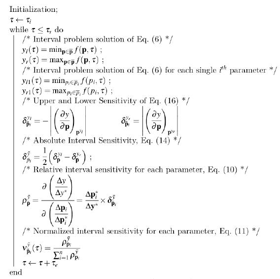
3.5 Interval Sensitivity Algorithm

This section presents the algorithm to analyze the uncertain interval structural response and the sensitivity of the flexible rotor as based on the numerical model and the interval approach (see Fig. 2).

Figure 2:
Interval Approach Algorithm.

The interval approach algorithm aims at computing the uncertain interval response and the correspondent sensitivity indices of the uncertain input parameters.

As mentioned, this approach is based on the global optimization method that demands for the solution of several global optimizations (Eq. (6)) at each time or frequency step ($\tau$) in which the dynamic response is analyzed. In the algorithm, $\tau$ varies from ${\tau }_i$ to ${\tau }_s$ with ${\tau }_e$ being the increment step. For this reason, this algorithm is time-consumming. Nevertheless, it can be easily implemented for the analysis of the flexible rotor system.

4 NUMERICAL RESULTS AND DISCUSSIONS

The flexible rotor considered in the present work for the interval uncertainty and sensitivity analysis is shown in Fig. 3. The rotor system is composed of a horizontal flexible steel shaft, modeled by 20 Euler-Bernoulli's beam elements, two rigid steel discs (D ₁ and D ₂ ), and three asymmetric bearings (B ₁ , B ₂ , and B ₃ ).

The geometrical and mechanical properties of the flexible rotor are presented in Table 1. The numerical model was implemented and simulated by using the Matlab/Simulink® platform. The model considered only the first six vibration modes of the rotor. The vibration responses are measured along the x and z directions at the position of the disc D ₁ for the analyses performed.

Figure 3:
Flexible rotor (Lara-Molina et al 2015).

Table 1:
Geometric and mechanical properties of the rotor elements (Lara-Molina et al 2015).

Rotor Element	Properties	Values
Shaft	Length [m] Diameter [m] Young’s modulus (E S ) [Pa] Density [kg/m3]	0.588 0.010 2x1011 7800
Disc D 1	Thickness [m] Diameter [m] Density [kg/m3]	0.005 0.150 7800
Disc D 2	Thickness [m] Diameter [m] Density [kg/m3]	0.010 0.150 7800
Bearings B 1, B 2 and B 3	kxx [N/m] k zz [N/m] c xx [Ns/m] c zz [Ns/m]	49000 60000 5 7
Proportional Damping $C_P=\alpha \left[M\right]+\beta \left[K\right]$	$\alpha$ $\beta$	1x10-1 1x10-5

The interval analysis described in section 3 was applied to the flexible rotor of Fig. 3 to assess its FRFs, orbits, Campbell diagram, and run-up responses in the presence of uncertain parameters. The uncertainty analysis consists in examining the system uncertain responses by solving typical optimization problems, as presented in Eq. (6).

Thus, the interval uncertainties were introduced in the Young's modulus of the shaft E _S and in the stiffness and damping coefficients of the bearings (B ₁ , B ₂ , and B ₃ ). Every single uncertain parameter is modeled as an interval that establishes upper and lower bounds, ${\acute{p}}_r$ and ${\acute{p}}_l$, respectively. It is worth mentioning that $\acute{p}=\left({\acute{p}}_l,{\acute{p}}_r\right)$ corresponds to the search space of the optimization problem defined by Eq. (6). In this case, ±5% of variation around the nominal value of the uncertain interval parameters was considered.

Different objective functions $f\left(p,\tau \right)$ were used both in the uncertain and sensitivity analyses dedicated to the rotor FRFs, orbits, Campbell diagram, and run-up responses. The interval FRF analysis was performed as based on the definitions of Eq. (2). Consequently, the optimization problem is stated as given by Eq. (16).

${y_l=\underset{p\in \acute{p}}{min}\left|{\widehat{H}\left(p,{\omega }_i\right)}^{-1}\right|y}_r=\underset{p\in \acute{p}}{max}\left|{\widehat{H}\left(p,{\omega }_i\right)}^{-1}\right|$ (16)

where ${\omega }_i$ is the frequency that varies between 0 and 250 Hz in steps of 1 Hz.

For the orbits, the instantaneous radius $r\left(t\right)=\sqrt{{x\left(t\right)}^2+{z\left(t\right)}^2}$ determined at the disc D ₁ was considered as an objective function. Thus, the optimization problem associated with the interval analysis was defined as follows:

${y_l=\underset{p\in \acute{p}}{min}r\left(p,t_i\right)y}_r=\underset{p\in \acute{p}}{max}r\left(p,t_i\right)$ (17)

where $t_i$ is the time that varies between 1 sec and 1.2 sec in steps of 0.002 sec.

For the Campbell diagram, two optimization problems were solved separately. In the first one, the first eigenfrequency ${\lambda }_1$ of the rotor, as obtained by the solution of the eigenvalue/eigenvector problem associated with Eq. (1), was defined as objective function. In the second optimization problem, the second eigenfrequency ${\lambda }_2$ of the rotor was adopted as objective function. Thus, the optimization problem used in the present interval analysis was defined as follows:

${y_l=\underset{p\in \acute{p}}{min}{\lambda }_j\left(p,{\Omega }_i\right)y}_r=\underset{p\in \acute{p}}{max}{\lambda }_j\left(p,{\Omega }_i\right)$ (18)

where j = 1, 2 and ${\Omega }_i$ is the rotating speed of the shaft, which varies from 0 to 8000 RPM in steps of 20 RPM.

Similar to the Campbell diagram analysis, two optimization problems were solved separately for the run-up condition regarding the vibration responses of the rotor along the x and z directions of the disc D ₁ . In this case, a linear run-up was considered for the shaft from 10 to 8000 RPM in 10 sec. Therefore, the optimization problem for this interval analysis was defined as follows:

$\begin{array}{c}{y_l=\underset{p\in \acute{p}}{min}{D}_{1x}\left(p,t_i\right)y}_r=\underset{p\in \acute{p}}{max}{D}_{1x}\left(p,t_i\right)\\ {y_l=\underset{p\in \acute{p}}{min}{D}_{1z}\left(p,t_i\right)y}_r=\underset{p\in \acute{p}}{max}{D}_{1z}\left(p,t_i\right)\end{array}$ (19)

where D _1x and D _1z are the vibration responses of the rotor along the x and z directions of the disc D ₁ , respectively. The time $t_i$ varies from 0 to 10 sec in steps of 0.125 sec.

The normalized interval sensitivity indexes are computed by following the algorithm presented in Fig. 2, which is based on the optimization problem for each considered analysis. The Differential Evolution (DE) algorithm (Price et al. 2006) was applied to solve the global optimization associated with the interval analyses of Eqs. (16)-(19). The parameters used in DE are described as follows: population size 10 per uncertain variable, 100 generations, crossover probability rate 0.8, perturbation rate 0.8, and the strategy adopted for the mutation mechanism is DE/rand/1/bin. These parameters are derived from the previous successful contributions (Lara-Molina et al. 2014; Lara-Molina et al. 2015).

4.1 Frequency Response Function

The objective function selected to evaluate the interval sensitivity is the norm $\left|H\left(\omega ,\Omega \right)\right|$ (see Eq. (2)) at the disc D ₁ (x direction). The interval FRF exhibits a small variation of the amplitude at the two first natural frequencies. Nevertheless, a considerable variation in the amplitude is found for frequencies close to 165 Hz.

Figure 4:
Interval FRF and sensitivity indices.

Figure 4(b) shows the normalized relative sensitivity indices for the uncertain interval FRF. Note that, the stiffness of the bearings along the x direction is the most sensitive parameter, i.e., k _x mostly contributes to the variation of the uncertain FRF amplitude. Nevertheless, a reduction of the sensitivity found for k _x is observed at the natural frequencies. The sensitivity of the damping of the bearings along the x direction (c _x ) increases at these natural frequencies. This behavior happens since the damping modulates the amplitude of the FRF at the natural frequencies.

The sensitivity of the bearing stiffness and damping coefficients along the z direction is negligible. These results were produced from the effect of gravity along the z direction. Finally, Young's modulus of the shaft exhibits a similar behavior of k _x , however with small sensitivity.

4.2 Orbits

In this case, the rotor is operating at 600 rpm to compute the orbits (Fig. 5(a)). This rotational speed is above the first and second natural frequencies. Consequently, the rotor operates distant from the critical speeds (see Campbell diagram of Fig. 6(a)). Figure 5(a) shows the uncertain interval orbit depicted in a polar reference frame. Note that the uncertain interval parameters of bearing stiffness and damping coefficients produce a significant variation in the orbit of disc D ₁ (see Fig. 5(b)).

Figure 5:
Interval orbit and sensitivity indices.

Figure 5(b) shows the normalized sensitivity indices. The most sensitive uncertain parameters are Young's modulus of shaft and stiffness coefficients of the bearings. However, the sensitivity of the uncertain parameters varies according to the polar position of the orbits. The stiffness of the bearings is more sensitive along their corresponding directions, i.e., k_x is more sensitive for polar positions in which the disc D ₁ moves along the x direction. The Young's modulus stiffness of the shaft exhibits a significant sensitivity that varies with the alternation of the sensitivity of k _x and k _z , respectively. Finally, the damping of bearings the c _x and c _z present small sensitivity with respect to the interval uncertain orbits.

4.3 Campbell Diagram

The Campbell diagram has been computed to investigate the effects of the uncertain interval parameters on the critical speeds of the flexible rotor (see Fig. 6(a)). Figure 6(b) shows the uncertain Campell diagrams for the two first critical velocities. A small effect of the uncertainties in the two critical speeds is observed in Fig. 4(a), which is in agreement with the results obtained for the FRF (see Fig. 4(a)).

Figure 6:
Campbell Diagram.

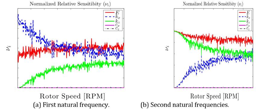
Regarding the first natural frequency (see Fig. 7(a)), the bearings stiffness bearing coefficients along the x direction is the most sensitive parameter and k _z has low sensitivity for small rotation speeds. Nevertheless, the sensitivity of k _x decreases and k _z becomes more sensitive as the speed increases. Additionally, the sensitivity of the stiffness is constant and the sensitivity of the damping is null because the natural frequencies do not depend on it.

For the second natural frequency (see Fig. 7(b)), the sensitivity of the stiffness of the bearing along the z direction is more sensitive for low rotation velocities differently from k _x whose sensitivity is null. With the increase of the rotational speed, the sensitivity of k _x also increases; however, the sensitivity of k _z decreases. The sensitivity of the stiffness of the shaft is almost constant and the sensitivity of the damping is almost null.

Figure 7:
Campbell Diagram: Sensitivity indices.

4.4 Run-up Response

Figure 8 shows the displacements along x and z directions at the disc D ₁ obtained for a linear run-up simulation (10 to 8000 rev/min in 10 sec). The first critical speed of the flexible rotor is, approximately, 1100 rev/min (as it can be seen in the Campbell diagram of Fig. 6). Additionally, the interval analysis was performed to evaluate the uncertain response by considering the horizontal and vertical displacements independently as objective functions (x(t) and z(t)). The uncertain parameters mainly influence the forth-critical speed, which is about 4200 RPM. At this rotation speed, the uncertain interval response is more disperse along the x direction (see Fig. 8(a)). Similarly, the greater dispersion of the uncertain interval run-up along the z direction is found in the vicinity of the critical speeds (see Fig. 8(b)).

Figure 8:
Run-Up.

Figure 9(b) exhibits the sensitivity indices of the uncertain parameter for the run-up in the range of the analyzed speeds (10 to 8000 rev/min). Figure 9(b) shows the sensitivity indices of the run-up along the x direction. The bearing stiffness along the x direction (k _x ) is more sensitive for speeds smaller than the third critical speed (3500 RPM), and k _z is more sensitive for speeds greater than the third critical speed. The stiffness of the shaft has an intermediate sensitivity for all the speeds considered. The bearing damping along the x direction c _x becomes more sensitive when the rotation speed is equal to critical speeds. The sensitivity of c _z is almost null.

The sensitivity indices along the run-up in the z direction are shown in Fig. 9(b). The sensitivity indices indicate that the stiffness of the shaft and bearings are more sensitive and the damping of the bearings presents a small sensitivity at the critical speeds.

Figure 9:
Run-Up: Sensitivity indices.

5 CONCLUSIONS

In this contribution both the uncertainty and sensitivity analyses of a flexible rotor system by using an interval approach was presented. The uncertain system response was computed by using the interval analysis together with the global optimization method. The sensitivity of each uncertain interval parameter was quantified by using sensitivity indices based on the interval analysis. The interval approach was successfully implemented in order to evaluate the time and frequency domain responses of the flexible rotor, which encompass the FRF, orbits, Campbell diagram and run-up responses.

The sensitivity analysis permitted the determination of the sensitivity for each uncertain parameter as a function either of time or frequency, i.e., this analysis allowed the evaluation of the sensitivity of each uncertain parameter as a function of time or frequency, respectively. The knowledge of the behavior of the sensitivity as obtained in this paper is useful for design and dynamic analysis purposes. Nevertheless, as a drawback of the application of the approach conveyed, the computation effort is heavy due to the use of the global optimization method to solve the optimization problems associated with the interval analysis.

For future works, the sensitivity analysis can also be used together with different procedures aiming at enhancing the robustness of rotor systems resulting from either robust optimal design or robust vibration control.

Acknowledgments

The authors are thankful for the financial support provided to the present research effort by CNPq (574001/2008-5, 304546/2018-8, 427204/2018-6 and 431337/2018-7), FAPEMIG (TEC-APQ-3076-09, TEC-APQ-02284-15, TEC-APQ-00464-16, and PPM-00187-18), and CAPES through the INCT-EIE.

References

• Arnst, M., Ponthot, J. P., & Boman, R. (2018). Comparison of stochastic and interval methods for uncertainty quantification of metal forming processes. Comptes Rendus Mécanique, 346(8), 634-646.
• Bachschmid, N. and Pennacchi, P. and Tanzi, E. (2010), “A sensitivity analysis of vibrations in cracked turbogenerator units versus crack position and depth”, Mechanical Systems and Signal Processing, 24(4), 844-859.
• Cavalini Jr, A. A. and Lara-Molina, F. A. and Sales, T. P. and Koroishi, E. H. and Steffen Jr, V. (2015), “Uncertainty analysis of a flexible rotor supported by fluid film bearings”, Latin American Journal of Solids and Structures, 12(8), 1487-1504.
• Didier, J. and Faverjon, B. and Sinou, J.J. (2012), “Analysing the dynamic response of a rotor system under uncertain parameters by polynomial chaos expansion”, Journal of Vibration and Control, 18(5), 712-732.
• Elishakoff, I. (1998). A comparison of stochastic and interval finite elements applied to shear frames with uncertain stiffness properties. Computers & structures, 67(1-3), 91-98.
• Genta, G. and De Lepine, X. and Impinna, F. and Girardello, J. and Amati, N. and Tonoli, A. (2011), “Sensitivity analysis of the design parameters in electrodynamic bearings”, IUTAM symposium on emerging trends in rotor dynamics, 287-296.
• Guo, J., & Du, X. (2009). Reliability sensitivity analysis with random and interval variables. International journal for numerical methods in engineering, 78(13), 1585-1617.
• Hickey, T. and Ju, Q. and Van, E., Maarten, H. (2001), “Interval arithmetic: From principles to implementation”, Journal of the ACM (JACM), 48(5), 1038-1068.
• Khatri, R. and Childs, D. W. (2015), “An Experimental Study of the Load-Orientation Sensitivity of Three-Lobe Bearings”, Journal of Engineering for Gas Turbines and Power, 137(4), 042503.
• Koroishi, E.H. and Lara-Molina, F.A. and Borges, A. S and Steffen Jr, V. (2016), “Robust control in rotating machinery using linear matrix inequalities”, Journal of Vibration and Control, 22(17), 3767-3778.
• Koroishi, E. and Cavalini Jr, A. A. and de Lima, A. M.G and Steffen Jr, V. (2012), “Stochastic modeling of flexible rotors”, Journal of the Brazilian Society of Mechanical Sciences and Engineering, 34(SPE2), 574-583.
• Lalanne, M. and Ferraris, G. (1998), Rotordynamics Prediction in Engineering, 2th edition, Wiley.
• Lara-Molina, F. A. and Koroishi, E. H. and Steffen Jr, V. (2015), “Uncertainty analysis of flexible rotors considering fuzzy parameters and fuzzy-random parameters”, Latin American Journal of Solids and Structures, 12(10), 1807-1823.
• Lara-Molina, F. A., Koroishi, E. H., & Steffen Jr, V. (2014). Análise estrutural considerando incertezas paramétricas fuzzy. Técnicas de Inteligência Computacional com Aplicações em Problemas Inversos de Engenharia. Omnipax, 1(1), 133-144.
• Lee, A. S. and Ha, J. W. (2003), “DDM Rotordynamic design sensitivity analysis of an APU turbo- generator having a spline shaft connection”, Journal of Mechanical Science and Technology, 17(1), 57-63.
• Leister, T. and Baum, C. and Seemann, W. (2016), “Sensitivity of Computational Rotor Dynamics Towards the Empirically Estimated Lubrication Gap Clearance of Foil Air Journal Bearings”, Proceedings in Applied Mathematics ans Mechanics, 16(1), 285-286.
• Modares, M. and Mullen, R. L. (2013), “Dynamic analysis of structures with interval uncertainty”, Journal of Engineering Mechanics, 140(4), 04013011.
• Moens, D. and Vandepitte, D. (2006), “Interval sensitivity analysis of dynamic response envelopes for uncertain mechanical structures”, III European Conference on Computational Mechanics, 385-385.
• Moens, D. and Vandepitte, D. (2007), “Interval sensitivity theory and its application to frequency response envelope analysis of uncertain structures”, Computer methods in applied mechanics and engineering, 196, 2486-2496.
• Möller, B. and Beer, M. (2013), Fuzzy randomness: uncertainty in civil engineering and computational mechanics, Springer Science & Business Media.
• Ben-Haim, Y. and Elishakoff, I. (2013), Convex models of uncertainty in applied mechanics, vol 25, Elsevier.
• Moore, R. E. and Kearfott, R. B. and Cloud, M. J. (2009), Introduction to interval analysis, vol 110, Siam.
• Ngo, V. T. and Xie, D. and Yang, Y. and Gao, S. and Guo, J. (2015), “Sensitivity Analysis on the Dynamic Characteristics of a 1000 MW Turbo-Generator Rotor”, Proceedings of the 9th IFToMM International Conference on Rotor Dynamics, 1841-1852.
• Price, K. and Storn, R. M and Lampinen, J. A. (2006), Differential evolution: a practical approach to global optimization, Springer Science & Business Media.
• Ritto, T.G. and Lopez, R.H. and Sampaio, R. and Souza de Cursi, J.E. (2011), “Robust optimization of a flexible rotor-bearing system using the Campbell diagram”, Engineering Optimization, 43(1), 77-96.
• Simões, R. C. and Steffen Jr, V. and Der Hagopian, J. and Mahfoud, J. (2007), “Modal active vibration control of a rotor using piezoelectric stack actuators”, Journal of Vibration and Control, 13(1), 45-64.
• Tamer, A. and Masarati, P. (2015), “Periodic stability and sensitivity analysis of rotating machinery”, Proceedings of the 9th IFToMM International Conference on Rotor Dynamics, 2059-2070.
• Urbiola-Soto, L. (2017), “Multivariate Response Rotordynamic Modeling and Sensitivity Analysis of Tilting Pad Bearings”, Journal of Engineering for Gas Turbines and Power, 140(7), 1301-1328.
• Walley, P. (1991), Statistical reasoning with imprecise probabilities, Chapman and Hall/CRC.
• Yan, S. and Sievert, R. (2015), “Vibration sensitivity of large turbine generator shaft trains to un- balance”, Proceedings of the 9th IFToMM International Conference on Rotor Dynamics, 3-14.
• Yin, S. and Wang, G. and Karimi, H. R. (2014), “Data-driven design of robust fault detection system for wind turbines”, Mechatronics, 24(4), 298-306.
• Zhang, Y.M. and Wen, B.C. and Liu, Q.L. (2013), “Reliability sensitivity for rotor-stator systems with rubbing”, Journal of Sound and Vibration, 259(5), 1095-1107.

Publication Dates

• Publication in this collection
  13 May 2019
• Date of issue
  2019

History

• Received
  01 Jan 2019
• Reviewed
  01 Mar 2019
• Accepted
  26 Mar 2019
• Published
  02 Apr 2019