A NURBS-based finite element formulation for incompressible fluid dynamics and fluid-structure interaction with rigid bodies

Abstract

A numerical investigation is performed here using a NURBS-based finite element formulation applied to classical Computational Fluid Dynamics (CFD) and Fluid-Structure Interaction (FSI) problems. Model capabilities related to refinement techniques are analyzed using a finite element formulation with NURBS (non uniform rational B-splines) basis functions, where B-splines and low-order Lagrangian elements can be considered as particular cases. An explicit two-step Taylor-Galerkin model is utilized for discretization of the fundamental flow equations and turbulence is considered using Large Eddy Simulation (LES) and the Smagorinsky’s sub-grid scale model. FSI is considered using an ALE kinematic formulation and a conservative partitioned coupling scheme with rigid body approach for large rotations is adopted. CFD and FSI applications are analyzed to evaluate the accuracy associated with the different refinement procedures utilized. Results show that high order basis functions with appropriate refinement and non-uniform parameterization lead to better predictions, compared with low-order Lagrangian models.

Keywords:
NURBS-based Finite Element Method; Computational Fluid Dynamics (CFD); Fluid-Structure Interaction; Large Eddy Simulation (LES); Rigid-body Dynamics; Arbitrary Lagrangian-Eulerian (ALE) Formulation

Graphical Abstract

1 INTRODUCTION

Although the use of finite volume models is still a common practice in the field of Computational Fluid Dynamics (CFD), the Finite Element Method (FEM) has gained some popularity in the last decades with significant advances observed in computers technology (see, for instance, Zienkiewicz et al., 2013; Reddy and Gartling, 2010). In the FEM context, the flow domain and the fundamental flow equations are spatially discretized using isoparametric finite elements with Lagrangian basis functions, where linear basis with C ⁰-continuity are usually adopted. However, the discretization procedure may lead to approximation errors, which may be significant depending on the geometrical characteristics of the physical model to be investigated. In addition, highly nonlinear and small-scale problems, especially turbulent flows, demand for high order discretization in both spatial and time domain. In order to overcome these drawbacks some improvements have been proposed to the finite element formulation, such as the use of NURBS (non uniform rational B-splines) basis functions, which are extensively utilized in Computational Aided Design (CAD) (see Piegl and Tiller, 1997). With this improvement, many possibilities with respect to refinement procedures may be conceived, in spite of some shortcomings that are also observed.

In the field of Engineering Design, computational reproduction of physical models has been traditionally performed using numerical tools based on CAD technologies, where NURBS are very popular. NURBS can exactly reproduce all conic sections and present convenient mathematical properties, such as C ^p-1-continuity order for p-degree basis functions, convex hull and variation diminishing properties (see, for instance, Piegl and Tiller, 1997). Recent advances have extended NURBS formulation by using T-splines (Sederberg et al., 2003), which permitted local refinement and compatibility of adjacent patches efficiently. By using NURBS functions in a finite element formulation, pre-processing and analysis procedures become unified, considering that the same numerical tools are employed.

However, when NURBS basis functions are utilized in finite element modeling, the numerical scheme must be reformulated in order to take into account a new framework for spatial interpolation. Basic concepts associated with control points and splines are introduced considering the formulation proposed in the automotive industry by De Casteljau and Bezier (see Townsend, 2014 for additional details), who utilized Bernstein polynomials and control points for manipulating geometric forms mathematically. De Casteljau observed that a curve could be accurately represented by manipulating some points around the curve and not along its length. By moving these points of influence (i.e., the control points), he noticed that the curve was modified such as moving weights in a boat builder spline. Later, the Bezier method was developed using similar concepts (see Bezier, 1972), which was surmounted by a recursive algorithm proposed by de Boor, where B-spline functions conceived by Schoenberg (1946) were adopted.

Other concepts were introduced with the B-spline functions, such as piecewise polynomials and knot vectors, which define the local support where a function is not null within the parametric space, considering that the parametric space is decomposed into knot spans by using breakpoints (knots). B-splines provide great flexibility for reproduction of geometries since the action of the control points is localized. In addition, B-splines can be seen as a generalization of Casteljau’s algorithm, including the Bezier method as a special case. Further improvements were obtained from the aerospace industry, where the existing methods were unable to handle with designing and assembling of aircraft components. NURBS were then conceived considering rational B-splines and knot vectors with non-uniform knot spans. By using control points with variable weighting, it was possible to draw conics exactly as well as reproduce complex curves and surfaces accurately (see Piegl and Tiller, 1997). NURBS-based finite element formulations have been widely applied to a variety of engineering problems, from solid mechanics (Espath et al., 2014; Espath et al., 2015) to material science (Gomez et al., 2008).

A NURBS finite element formulation for CFD applications presents significant improvements over the classical Lagrangian finite element formulation. Complex flow phenomena, such as boundary layer and turbulent flows, separation, and reattachment are better reproduced considering that different flow regions can be discretized using distinct combinations of degree and continuity order associated with the interpolation functions. These basis functions are always smooth (C ^∞) within the knot span and are C ^p-m continuous at the knots, where p is the polynomial degree and m is the knot multiplicity. Nevertheless, NURBS basis functions are not interpolatory in general since the control mesh defined by the control points does not conform to the actual geometry of the physical model. Notice that flow variables and coordinates are defined at the control points. The flow spatial domain may be decomposed into patches, depending on its geometric complexity, where independent parametric spaces are adopted considering that they must be compatible on patch interfaces. Every patch is also decomposed into knot spans, which define the element concept in a NURBS-based finite element formulation. Most of the classical flow problems can be simulated using a single patch, although multiple patches can also be utilized in order to obtain a more efficient discretization. Finite element formulations with NURBS basis functions applied to CFD and FSI problems may be found in Bazilevs et al. (2006), Gomez et al. (2010), Nielsen et al. (2011), Akkerman et al. (2011), and Kadapa et al. (2015).

Unlike the standard finite element refinement techniques, B-spline refinement can control element size as well as degree and continuity order of the basis functions. The basic refinement techniques associated with B-splines are knot insertion and degree elevation, which do not change the physical model geometrically or parametrically. By using knot insertion, the solution space is enriched with additional elements, control points, and basis functions, but without changing the geometry. Knot insertion is equivalent to h-refinement adopted in the finite element modeling only when knots are inserted with multiplicity m = p in order to maintain the basis functions with C ⁰ continuity. In general, knots can be inserted with multiplicity m = 1, maintaining the original continuity of the basis functions, independently of the polynomial degree. This aspect cannot be replicated with a standard finite element formulation.

When order elevation is performed, knot multiplicity of the existing knots is also increased in order to maintain the original continuity order of the basis functions along the element boundaries and no new knots are created. Notice that the classical p-refinement utilized in finite element modeling must be initially applied over basis functions with C ⁰-continuity, while p-refinement for B-spline discretizations can be adopted using any continuity order. This aspect cannot be replicated with a standard finite element formulation. An exclusive technique for B-spline refinement is obtained by using degree elevation followed by knot insertion, which is called k-refinement. One can notice that a NURBS-based finite element formulation becomes highly flexible with respect to continuity order of the basis functions and other refinement methods can be devised. Additional information on refinement methods for finite element formulations with NURBS basis functions are found in Cottrell et al. (2009).

In this work, a NURBS-based finite element formulation is proposed considering the explicit two-step Taylor-Galerkin model, where spatial discretization is carried out taking into account B-splines and NURBS basis functions. The fundamental flow equations are the Navier-Stokes equations and the mass conservation equation, which is described according to the pseudo-compressibility hypothesis for incompressible flows and Newtonian fluids under isothermal conditions. In the present model, idealized 2D turbulent flows are simulated using a LES-type (Large Eddy Simulation) approach, where the Smagorinsky’s model is adopted for sub-grid scale modeling. Fluid-structure interaction (FSI) problems are reproduced using a conservative partitioned coupling model and a rigid body approach for large rotations. Finally, classical CFD and FSI applications are analyzed in order to validate the present methodology, where different refinement procedures are adopted and investigated.

2 FUNDAMENTAL EQUATIONS

2.1 Flow analysis

In the present model, the flow analysis is performed considering the following assumptions: fluid particles are described constitutively according to the Newtonian model for viscous fluids, and the flow is two-dimensional and restricted to the incompressible regime under isothermal conditions. In addition, fluid body forces are neglected and a mixed approach is adopted for variables definition, where the pressure field is explicitly evaluated using the pseudo-compressibility hypothesis (see Chorin, 1967). An Arbitrary Lagrangian-Eulerian (ALE) formulation is adopted for the kinematical description of fluid motions when fluid-structure interaction is considered, and turbulence flows are approximately reproduced using Large Eddy Simulation (LES) and the Smagorinsky’s sub-grid scale model (Smagorinsky, 1963). Thus, the system of fundamental flow equations may be written as follows (see, for instance, White, 2005):

Momentum balance equation

$\frac{\partial v_i}{\partial t}+\left(v_j+w_j\right)\frac{\partial v_i}{\partial x_j}=\frac{1}{\rho }\frac{\partial }{\partial x_j}\left({\sigma }_{ij}+{\tau }_{ij}^{SGS}\right)\left(i,j=\mathrm{1,2}\right)in{\Omega }^f$ (1)

Mass balance equation

$\frac{\partial p}{\partial t}+\rho c^2\frac{\partial v_j}{\partial x_j}=0(j=\mathrm{1,2})in{\Omega }^f$ (2)

where v_i and w_i are the components of the flow velocity vector v and mesh velocity vector w, respectively, which correspond to the i-direction of a rectangular Cartesian coordinates system, where coordinates components are denoted by x_i, p is the thermodynamic pressure, ρ is the fluid specific mass and c is the sound speed in the flow field. Although the sound speed c usually has a strict physical meaning, this parameter is considered here as a numerical parameter in order to satisfy the incompressible flow condition (divergence-free velocity field). The fundamental flow equations are valid in the flow spatial domain Ω^f, which is bounded by ${\Gamma }_t^{Tf}$at a time instant t, with t ∈ [0, T], where the subscript t indicates time dependence on the spatial domain during the time interval [0, T].

The fluid stress tensor σ is given according to the Newtonian constitutive model for viscous fluids, that is:

${\sigma }_{ij}=-p{\delta }_{ij}+{\tau }_{ij}\left(i,j=\mathrm{1,2}\right)$ (3)

with:

${\tau }_{ij}=\mu \left(\frac{\partial v_i}{\partial x_j}+\frac{\partial v_j}{\partial x_i}\right)+\lambda \frac{\partial v_k}{\partial x_k}{\delta }_{ij}\left(i,j,k=\mathrm{1,2}\right)$ (4)

where μ and λ are the dynamic and volumetric viscosities of the fluid and δ_ij are the components of the Kroenecker’s delta (δ_ij = 1 for i = j; δ_ij = 0 for i ≠ j).

Idealized turbulence flows are simulated here using a LES-type approach, where the fundamental flow equations are submitted to spatial filtering in which the flow field is decomposed into large and small-scale components. Large scales are solved directly utilizing the filtered equations, while scales smaller than the mesh resolution are defined by the sub-grid stress tensor τ^SGS, which must be modeled considering a turbulence closure model. Turbulence models are utilized in order to represent the small-scale effects over the large scales. The sub-grid stress tensor components ${\tau }_{ij}^{SGS}$ are usually approximated according to the Boussinesq assumption, that is:

${\tau }_{ij}^{SGS}=2{\mu }_t{\overline{S}}_{ij}\left(i,j=\mathrm{1,2}\right)$ (5)

where ${\overline{S}}_{ij}$ are components of the filtered strain rate tensor. In the present work, eddy viscosity μ_t is obtained considering the Smagorinsky’s sub-grid scale model, which may be expressed as follows:

${\mu }_t=\rho C_S\overline{\Delta }\left|\overline{S}\right|$ (6)

where C_S is the Smagorinsky constant, which must be specified according to the flow characteristics, with values usually ranging from 0.1 to 0.25, and $\overline{\Delta }$ is the characteristic length of the spatial filter, which may be locally defined as $\overline{\Delta }=\sqrt{{\Omega }_E}$ for a box filter (see Smagorinsky, 1963 for additional details), where Ω_E is the finite element area referring to element E. When laminar flows are investigated, the sub-grid stress tensor components ${\tau }_{ij}^{SGS}$ are omitted in Eq. (1). It is important to notice that the present approach is only an approximation of the actual LES, considering that a turbulent flow is inherently three-dimensional.

In order to solve the flow problem, initial conditions on the flow variables v_i and p must be specified. In addition, appropriate boundary conditions must also be defined on ${\Gamma }_t^{Tf}$, which may be expressed as:

$v_i=w_i(i=\mathrm{1,2})on{\Gamma }_t^{fsi}$ (7)

$v_i={\tilde{v}}_i(i=\mathrm{1,2})on{\Gamma }^v$ (8)

$p=\tilde{p}on{\Gamma }^p$ (9)

${\sigma }_{ij}{n}_j=\left[-p{\delta }_{ij}+{\tau }_{ij}\right]n_j={\tilde{t}}_i(i=\mathrm{1,2})on{\Gamma }^{\sigma }$ (10)

where ${\Gamma }_t^{fsi}$ (boundary representing the fluid-structure interface), ${\Gamma }^v$ (boundary with prescribed velocity ${\tilde{v}}_i$), ${\Gamma }^p$ (boundary with prescribed pressure $\tilde{p}$) and ${\Gamma }^{\sigma }$ (boundary with prescribed traction ${\tilde{t}}_i$) are complementary subsets of ${\Gamma }_t^{Tf}$, such that ${\Gamma }_t^{Tf}$= ${\Gamma }_t^{fsi}$∪${\Gamma }^v$∪${\Gamma }^p$∪${\Gamma }^{\sigma }$. In Eq. (10), nj are components of the unit normal vector n evaluated at a point on boundary ${\Gamma }^{\sigma }$. Notice that wi = 0 for points outside the ALE domain or when motions of the immersed body are not considered in the flow analysis.

2.2 Fluid-structure interaction

The fluid-structure coupling is accomplished by enforcing equilibrium and kinematical conditions on the fluid-structure interface ${\Gamma }_t^{fsi}$. The no-slip condition is assumed for viscous fluids, such that the relative velocity of fluid particles on the fluid-structure interface is set to zero. In this case, the equilibrium and compatibility equations may be expressed as follows:

$t_i^s=\left[-p{\delta }_{ij}+{\tau }_{ij}\right]n_j(i,j=\mathrm{1,2})on{\Gamma }_t^{fsi}$ (11)

$u_i^s=u_i^f(i=\mathrm{1,2})on{\Gamma }_t^{fsi}$ (12)

where n_j and $t_i^s$ are components of the unit normal vector n and the structure traction vector t ^s evaluated at a point on boundary ${\Gamma }_t^{fsi}$ and $u_i^s$ and $u_i^f$ are components of the structure and fluid displacement vectors u ^s and u ^f corresponding to a point belonging to the fluid-structure interface ${\Gamma }_t^{fsi}$. In addition, continuity conditions are also imposed on ${\Gamma }_t^{fsi}$ when moving grids are adopted, which may be given as follows:

$x_i=u_i^s(i=\mathrm{1,2})on{\Gamma }_t^{fsi}$ (13)

$\frac{\partial x_i}{\partial t}=\frac{\partial u_i^s}{\partial t}(i=\mathrm{1,2})on{\Gamma }_t^{fsi}$ (14)

where x_i are components of the mesh position vector x referring to the flow spatial domain.

In order to solve the flow problem on moving grids adequately, the geometric conservation law (GCL) must be satisfied (see Thomas and Lombard, 1979 for further information). According to Lesoinne and Farhat (1996), the GCL is satisfied in ALE finite element formulations if the mesh velocity vector w is calculated as:

$w=\dot{x}=\frac{x_{n+1}-x_n}{\Delta t}$ (15)

Considering that the trapezoidal form of the Newmark’s method is utilized for solving the structural equation of motion and a partitioned algorithm is adopted for fluid-structure coupling, a conservative algorithm where the GCL is satisfied without violating the compatibility conditions can be obtained if the following equations are employed (seeLesoinne and Farhat, 1998):

$x_{n+1/2}=x_{n-1/2}+\Delta t{\dot{x}}_{n}on{\Gamma }_t^{fsi}$ (16)

where:

${\dot{x}}_n={\dot{u}}_n^{s}on{\Gamma }_t^{fsi}$ (17)

${\dot{x}}_{n-1/2}=u_n^s-\frac{\Delta t}{2}{\dot{u}}_n^{s}on{\Gamma }_t^{fsi}$ (18)

Figure 1 shows the coupling scheme adopted here for fluid-structure interaction problems, where one can observe that the flow and structure analyses are performed sequentially. In addition, it is also observed that fluid and structure are displaced in time by a half time step Δt/2.

Figure 1
Coupling scheme for the conservative partitioned model.

The mesh motion must be arbitrarily defined when ALE formulation is adopted for the kinematical description of the fluid flow. In this work, a mesh motion scheme utilized by Braun and Awruch (2009) is employed, where the mesh velocity field is obtained as follows:

$w_k^i=\frac{{\displaystyle \sum _{j=1}^{NS}{a}_{ij}{w}_k^j}}{{\displaystyle \sum _{j=1}^{NS}{a}_{ij}}}(k=\mathrm{1,2})$ (19)

where NS is the number of mesh points located on the boundaries of the ALE domain and a_ij are influence coefficients defined with mesh points i and j, considering that i are inner mesh points and j are mesh points belonging to the boundaries of the ALE domain, where w_i = 0. The influence coefficients are obtained with:

$a_{ij}=\frac{1}{{\left(d_{ij}\right)}^n}$ (20)

where d_ij is the Euclidian distance between the mesh points i and j and exponent n is a user-defined parameter, which is chosen according to the amplitude of the immersed body displacements. In this work, all FSI applications were analyzed using n = 4.

The structural response is obtained here considering the equation of motion for two-dimensional rigid bodies with elastic constraints and viscous dampers, which may be expressed as:

$M^s{\ddot{U}}_c^s+C^s{\dot{U}}_c^s+K^s{U}_c^s=Q_c^s$ (21)

where M ^s is the mass matrix, C ^s is the damping matrix, K ^s is the stiffness matrix and ${\ddot{U}}_c^s$, ${\dot{U}}_c^s$ and $U_c^s$ are the acceleration, velocity and displacement vectors evaluated at the center of mass of the structure, which are written using three degrees of freedom, with two translational displacements and one rotational displacement. The load vector applied at the center of mass of the structure is denoted by $Q_c^s$, with two force components and one moment component. Notice that s and c indicate that quantity refers to structure and center of mass, respectively.

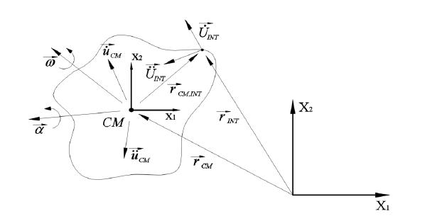
The structural motion on the fluid-structure interface is obtained from the structural response evaluated at the center mass by considering the following kinematic relations (see Figure 2):

${\dot{u}}_{\mathrm{int}}^s={\dot{u}}_c^s+{\omega }^s\times r_{c,\mathrm{int}}$ (22)

${\ddot{u}}_{\mathrm{int}}^s={\ddot{u}}_c^s+{\alpha }^s\times r_{c,\mathrm{int}}+{\omega }^s\times \left({\omega }^s\times r_{c,\mathrm{int}}\right)$ (23)

Figure 2
Kinematic relations between center of mass and the fluid-structure interface.

where ${\dot{u}}_{\mathrm{int}}^s$ and ${\ddot{u}}_{\mathrm{int}}^s$ are the velocity and acceleration vectors evaluated at a point on the fluid-structure interface, r _c,int is the position vector referring to a point on the fluid-structure interface with respect to the center of mass of the structure, ω ^s is the vector of angular velocity and α ^s is the vector of angular acceleration.

The kinematic relations above may also be expressed using matrix form, that is:

${\dot{U}}_{\mathrm{int}}^s=L{\dot{U}}_c^s$ (24)

${\ddot{U}}_{\mathrm{int}}^s=L{\ddot{U}}_c^s+L^{\prime }{\dot{U}}_c^s$ (25)

where:

$L=\left[\begin{array}{lll}1\hfill & 0\hfill & -r_2\hfill \\ 0\hfill & 1\hfill & r_1\hfill \end{array}\right]L^{\prime }=\left[\begin{array}{lll}0\hfill & 0\hfill & -{\omega }_3{r}_1\hfill \\ 0\hfill & 0\hfill & -{\omega }_3{r}_2\hfill \end{array}\right]$ (26)

$L=\left[\begin{array}{lll}1\hfill & 0\hfill & -r_2\hfill \\ 0\hfill & 1\hfill & r_1\hfill \end{array}\right]L^{\prime }=\left[\begin{array}{lll}0\hfill & 0\hfill & -{\omega }_3{r}_1\hfill \\ 0\hfill & 0\hfill & -{\omega }_3{r}_2\hfill \end{array}\right]$ (27)

${\dot{U}}_{\mathrm{int}}^s=\left[\begin{array}{c}{\dot{u}}_{\mathrm{1,}\mathrm{int}}^s\\ {\dot{u}}_{\mathrm{2,}\mathrm{int}}^s\end{array}\right]{\dot{U}}_c^s=\left[\begin{array}{c}{\dot{u}}_{\mathrm{1,}c}^s\\ {\dot{u}}_{\mathrm{2,}c}^s\\ {\omega }_3\end{array}\right]{\ddot{U}}_{fsi}^s=\left[\begin{array}{c}{\ddot{u}}_{\mathrm{1,}\mathrm{int}}^s\\ {\ddot{u}}_{\mathrm{2,}\mathrm{int}}^s\end{array}\right]{\ddot{U}}_c^s=\left[\begin{array}{c}{\ddot{u}}_{\mathrm{1,}c}^s\\ {\ddot{u}}_{\mathrm{2,}c}^s\\ {\alpha }_3\end{array}\right]$ (28)

The fluid forces acting on the structure are obtained considering the equilibrium condition imposed on the fluid-structure interface. This load must be transferred to the center of mass of the structure in order to solve the equation of motion for rigid bodies. This procedure may be carried out using the following expressions (see Figure 3):

$Q_{fsi}^s=-{\displaystyle \underset{{\Gamma }_{fsi}}{\int }{t}_{\mathrm{int}}^f}d\Gamma$ (29)

$Q_c^s=-{\displaystyle \underset{{\Gamma }_{fsi}}{\int }{L}^T{t}_{\mathrm{int}}^f}d\Gamma$ (30)

where $t_{\mathrm{int}}^f$ is the fluid traction vector, which is evaluated using Eq. (10) for a point located at the fluid-structure interface, where the translation matrix L given by Eq. (26) is also evaluated.

Figure 3
Equilibrium conditions on the fluid-structure interface.

3 NUMERICAL MODEL

3.1 NURBS-based finite element formulation

In a NURBS-based finite element formulation for fluid dynamics the spatial domain is initially decomposed into patches according to the geometric complexity of the problem investigated, where the basis functions are defined using individual parametric spaces. In order to define the element concept in the present formulation, every patch is divided into knots spans specified in the different directions of the parametric space by using the knot vectors (seeFigure 4). For two-dimensional problems, the following knot vectors may be utilized:

$\Xi \left(\xi \right)=\left\{\underset{p+1}{\underbrace{\mathrm{0,...,0}}},{\xi }_{p+1}\mathrm{,...,}{\xi }_{s_p-p-1},\underset{p+1}{\underbrace{\mathrm{1,...,1}}}\right\}with{s}_p=n+p+1$ (31)

$\Psi \left(\eta \right)=\left\{\underset{p+1}{\underbrace{\mathrm{0,...,0}}},{\eta }_{q+1}\mathrm{,...,}{\eta }_{s_q-q-1},\underset{p+1}{\underbrace{\mathrm{1,...,1}}}\right\}with{s}_q=m+q+1$ (32)

where p and q are the polynomial degrees of the basis functions defined over the parametric directions ξ and η, respectively. The number of basis functions associated with the parametric directions ξ and η is defined by n+1 and m+1, respectively, which also defines the corresponding number of control points, and the number of elements is determined by the number of non-zero knot spans.

The NURBS basis functions for two-dimensional applications are given by:

$R_{i,j}^{p,q}\left(\xi ,\eta \right)=\frac{N_{i,p}\left(\xi \right)N_{j,q}\left(\eta \right)w_{i,j}}{{\displaystyle \sum _{\widehat{i},\widehat{j}}^{n,m}{N}_{\widehat{i},p}\left(\xi \right)N_{\widehat{j},q}\left(\eta \right)w_{\widehat{i},\widehat{j}}}}$ (33)

where the subscripts i and j indicate the position of the control point in the index space and the superscripts p and q denote the polynomial degree of the basis functions. The weight term w_i,j is related to the weight associated with the control point defined by the subindices i and j. The B-spline basis functions N_i are evaluated here using the Cox-de Boor recursive formulation (Cox, 1972; De Boor, 1972), which may be expressed as:

$\begin{array}{l}{N}_{i\mathrm{,0}}\left(\xi \right)=\{\begin{array}{ll}1\hfill & if{\xi }_i\le \xi <{\xi }_{i+1}\hfill \\ 0\hfill & otherwise\hfill \end{array}\\ N_{i,p}\left(\xi \right)=\frac{\xi -{\xi }_i}{{\xi }_{i+p}-{\xi }_i}{N}_{i,p-1}\left(\xi \right)+\frac{{\xi }_{i+p+1}-\xi }{{\xi }_{i+p+1}-{\xi }_{i+1}}{N}_{i+\mathrm{1,}p-1}\left(\xi \right)\end{array}$ (34)

where p is the polynomial degree of the basis function N(ξ) and i is the knot index. Notice that Eq. (34) is straightforwardly extended to basis functions associated with the parametric direction η.

Figure 4
Definitions on spatial discretization using a NURBS-based finite element formulation.

Considering that n+1 and m+1 denote the number of basis functions related to the parametric directions ξ and η, respectively, and the respective polynomial degrees are defined by p and q, element e is identified by determining the indices at which the corresponding non-zero knot span begins in the index space, that is:

$e=\left[{\xi }_i,{\xi }_{i+1}\right]\times \left[{\eta }_i,{\eta }_{i+1}\right]$ (35)

where p+1 ≤ i ≤ n and q+1 ≤ j ≤ m. The total number of elements in which the spatial field is discretized in the parametric domain is defined as:

$n_{el}=\left(n-p+1\right).\left(m-q+1\right)$ (36)

Finally, geometry and flow variables are discretized using the following NURBS approximations:

$x\left(\xi ,\eta ,t\right)={\displaystyle \sum _{i=1}^{ncp}{R}_i\left(\xi ,\eta \right)x_i\left(t\right)}$ (37)

$v\left(\xi ,\eta ,t\right)={\displaystyle \sum _{i=1}^{ncp}{R}_i\left(\xi ,\eta \right)v_i\left(t\right)}\delta v\left(\xi ,\eta ,t\right)={\displaystyle \sum _{i=1}^{ncp}{R}_i\left(\xi ,\eta \right)\delta v_i\left(t\right)}$ (38)

$p\left(\xi ,\eta ,t\right)={\displaystyle \sum _{i=1}^{ncp}{R}_i\left(\xi ,\eta \right)p_i\left(t\right)}\delta p\left(\xi ,\eta ,t\right)={\displaystyle \sum _{i=1}^{ncp}{R}_i\left(\xi ,\eta \right)\delta p_i\left(t\right)}$ (39)

where R_i is the NURBS basis function related to control point i, which is defined as a function of the parametric coordinates (ξ,η), and ncp is the number of global control points (or basis functions). The control point variables and geometry are specified by v _i, δv _i, p, δp and x _i. Notice that the sum operations indicated above are performed over the total number of basis functions available (ncp), considering that basis functions support is highly localized.

3.2 The explicit two-step Taylor-Galerkin model

In the present model, the fundamental flow equations are discretized using the explicit two-step Taylor-Galerkin model, where second-order Taylor series and the Bubnov-Galerkin method are adopted for time and space discretization considering a NURBS-based finite element framework.

Time discretization is initially applied to the fundamental flow equations considering a second-order Taylor series expansion and a two-step time increment scheme, which leads to the following formulation:

$v_i^{n+1}=v_i^n+\Delta v_i^{n+1/2}$ (40)

$p^{n+1}=p^n+\Delta p^{n+1/2}$ (41)

where:

$\Delta v_i^{n+1/2}=\Delta t{\left\{\frac{\partial }{\partial x_j}\left[\left(\frac{\mu +{\mu }_t}{\rho }\right)\left(\frac{\partial v_i}{\partial x_j}+\frac{\partial v_j}{\partial x_i}\right)+\frac{\lambda }{\rho }\frac{\partial v_k}{\partial x_k}{\delta }_{ij}\right]-\left(v_j-w_j\right)\frac{\partial v_i}{\partial x_j}-\frac{1}{\rho }\frac{\partial p}{\partial x_j}{\delta }_{ij}\right\}}^{n+1/2}$ (42)

$\Delta p^{n+1/2}=-\Delta t{\left[\rho c^2\frac{\partial v_j}{\partial x_j}\right]}^{n+1/2}$ (43)

where Δt is the time increment. Notice that the flow variables must be evaluated at n+1/2 in order to obtain the velocity and pressure increments defined by Eqs. (42) and (43). The velocity and pressure fields at n+1/2 are obtained from:

$\begin{array}{l}{\tilde{v}}_i^{n+1/2}=v_i^n+\frac{\Delta t}{2}\{\frac{\partial }{\partial x_j}\left[\left(\frac{\mu +{\mu }_t}{\rho }\right)\left(\frac{\partial v_i}{\partial x_j}+\frac{\partial v_j}{\partial x_i}\right)+\frac{\lambda }{\rho }\frac{\partial v_k}{\partial x_k}{\delta }_{ij}\right]-\left(v_j-w_j\right)\frac{\partial v_i}{\partial x_j}-\\ {\frac{1}{\rho }\frac{\partial p}{\partial x_j}{\delta }_{ij}+\frac{\Delta t}{4}\left(v_j-w_j\right)\left(v_k-w_k\right)\frac{{\partial }^2{v}_i}{\partial x_j\partial x_k}\}}^n\end{array}$ (44)

$p^{n+1/2}=p^n-\frac{\Delta t}{2}{\left[\rho c^2\frac{\partial v_j}{\partial x_j}\right]}^n$ (45)

The velocity field at n+1/2 must be corrected considering that a pressure increment term was omitted in Eq. (44). The velocity correction is performed using the following equation:

$v_i^{n+1/2}={\tilde{v}}_i^{n+1/2}-\frac{1}{\rho }\frac{\Delta t}{4}\frac{\partial \Delta p^{n+1/2}}{\partial x_j}{\delta }_{ij}$ (46)

The weighted residual principle is adopted here in order to minimize approximation errors associated with geometry and flow variables, which may be written here as follows:

${\displaystyle \sum _{e=1}^{nel}\left({\displaystyle \underset{{\Omega }_e}{\int }{W}_v^T{R}_{v}d\Omega }\right)}$ (47)

${\displaystyle \sum _{e=1}^{nel}\left({\displaystyle \underset{{\Omega }_e}{\int }{W}_p^T{R}_{p}d\Omega }\right)}$ (48)

where Ω_e is spatial domain referring to element e and nel is the number of elements in the finite element mesh. R _vandR _p are the residual vectors referring to the momentum and mass balance equations, respectively, which are obtained by approximating the flow variables and geometry with the finite element interpolations given by Eqs. (37), (38) and (39). By using the Bubnov-Galerkin method, the weight functions are defined here using W _v = δv and W _p = δp, which are also approximated using velocity and pressure variations given by Eqs. (38) and (39). In order to reduce continuity requirements over the basis functions, the weak form of the flow formulation is adopted using the Green-Gauss theorem. An algebraic system of equations is obtained for the two-step Taylor-Galerkin model utilized in this work, where the flow variables are first evaluated at n+1/2 with the following expressions:

$M{\tilde{v}}_i^{n+1/2}=M{v}_i^n+\frac{\Delta t}{2}{\left[t_i-\left(A+B\right)v_i-\frac{1}{\rho }{G}_j{\delta }_{ij}p-D_{ij}{v}_j\right]}^n$ (49)

$M{p}^{n+1/2}=M{p}^n-\frac{\Delta t}{2}{\left[\rho c^2{G}_j^T{v}_j\right]}^n$ (50)

The velocity field is then corrected with:

$M{v}_i^{n+1/2}=M{\tilde{v}}_i^{n+1/2}-\frac{1}{\rho }\frac{\Delta t}{4}{G}_j^T\left(p^{n+1/2}-p^n\right){\delta }_{ij}$ (51)

Finally, the flow variables at n+1 are obtained using:

$M{v}_i^{n+1}=M{v}_i^n+\Delta t{\left[t_i-A{v}_i-\frac{1}{\rho }{G}_j{\delta }_{ij}p-D_{ij}{v}_j\right]}^{n+1/2}$ (52)

$M{p}^{n+1}=M{p}^n-\Delta t{\left[\rho c^2{G}_j^T{v}_j\right]}^{n+1/2}$ (53)

where M is the fluid mass matrix, G is the gradient matrix, A is the advection matrix, D is the diffusion matrix and B is the balance diffusivity tensor. Detailed information on the two-step Taylor-Galerkin scheme may be found in Kawahara and Hirano (1983).

The element matrices are numerically evaluated using Gaussian quadrature, where three different spaces are considered: the physical space Ω_e, which is defined by the vector of Cartesian coordinates x = (x₁, x₂); the parametric space ${\widehat{\Omega }}_e$, which is defined by the vector of parametric coordinates ξ = (ξ,η) and the quadrature space ${\tilde{\Omega }}_e$, which is defined by the vector of quadrature space coordinates $\tilde{\xi }=\left(\tilde{\xi },\tilde{\eta }\right)$. The mapping from physical to quadrature space is performed using the Jacobian transformation matrix as follows:

$\frac{dx}{d\tilde{\xi }}=\frac{dx}{d\xi }\frac{d\xi }{d\tilde{\xi }}$ (54)

The parametric and quadrature spaces are related according to the following equations:

$\xi ={\xi }_i+\left(\tilde{\xi }+1\right)\frac{\left({\xi }_{i+1}+{\xi }_i\right)}{2}$ (55)

$\eta ={\eta }_i+\left(\tilde{\eta }+1\right)\frac{\left({\eta }_{i+1}+{\eta }_i\right)}{2}$ (56)

where the parametric space referring to element e is defined by ${\widehat{\Omega }}_e=\left[{\xi }_i,{\xi }_{i+1}\right]\times \left[{\eta }_i,{\eta }_{i+1}\right]$.

The time increment Δt is locally determined using the Courant’s stability condition, that is:

$\Delta t_e=\alpha \frac{\Delta x_e}{c+v_e}$ (57)

where Δt_e is the time increment referring to element e, α is the safety coefficient (0 ≤ α ≤ 1), Δx_e is the characteristic length of element e, c is the sound speed, and v_e is the flow characteristic speed. Although a multi time step formulation may be adopted for time integration, the smaller Δt_e is utilized in this work throughout the finite element mesh.

3.3 Fluid-structure coupling model

In the present work, a conservative partitioned model is adopted for fluid-structure coupling. Considering a fluid element Ω_E localized on the fluid-structure interface, the discretized momentum equation referring to element E may be written as:

$M^f\dot{v}+A^{f}v+D^{f}v-\frac{1}{\rho }{G}^{f}p=\frac{1}{\rho }F$ (58)

This equation is rearranged in order to define mesh points of element E belonging to the fluid-structure interface (I) and mesh points located within the fluid flow domain (F). A matrix form of the rearranged system may be expressed as:

$\left[\begin{array}{cc}{M}_{II}^f& M_{IF}^f\\ M_{FI}^f& M_{FF}^f\end{array}\right]\left\{\begin{array}{c}{\dot{v}}_I\\ {\dot{v}}_F\end{array}\right\}+\left[\begin{array}{cc}{A}_{II}^f+D_{II}^f& A_{IF}^f+D_{IF}^f\\ A_{FI}^f+D_{FI}^f& A_{FF}^f+D_{FF}^f\end{array}\right]\left\{\begin{array}{c}{v}_I\\ v_F\end{array}\right\}-\frac{1}{\rho }\left[\begin{array}{cc}{G}_I^f& 0\\ 0& G_I^f\end{array}\right]\left\{\begin{array}{c}{p}_I\\ p_F\end{array}\right\}=\frac{1}{\rho }\left\{\begin{array}{c}{F}_I\\ F_F\end{array}\right\}$ (59)

One can notice that only the first line of the system of equations above is relevant for the fluid-structure problem. In addition, the compatibility conditions are also expressed in matrix form considering an element E belonging to the fluid-structure interface as follows:

$v_I={\dot{U}}_{\mathrm{int}}^s=T{\dot{U}}_c^s$ (60)

${\dot{v}}_I={\ddot{U}}_{\mathrm{int}}^s=T{\ddot{U}}_c^s+T^{\prime }{\dot{U}}_c^s$ (61)

where:

$T=\left[\begin{array}{c}{L}_1\\ L_2\\ ⋮\\ L_N\end{array}\right]T^{\prime }=\left[\begin{array}{c}{L^{\prime }}_1\\ {L^{\prime }}_2\\ ⋮\\ {L^{\prime }}_N\end{array}\right]$ (62)

Notice that N is the number of mesh points referring to element E and the matrices L _i and L’_i associated with mesh points out of the fluid-structure interface are set to zero.

The load vector at the center of mass of the structure is obtained considering the equilibrium equation, which may be defined as:

$Q_c^s=-\rho T^T{F}_I$ (63)

where F _I is the fluid force vector corresponding to the first row of the system of equations given by Eq. (59). By substituting Eq. (59) into Eq. (63), one obtains the following expression:

$\begin{array}{l}{Q}_c^s=-\{\rho T^T{M}_{II}^f{\dot{v}}_I+\rho T^T{M}_{IF}^f{\dot{v}}_F+\\ T^T\left[\rho \left(A_{II}^f+D_{II}^f\right)v_I+\rho \left(A_{IF}^f+D_{IF}^f\right)v_F-G_I^f{p}_I\right]\}\end{array}$ (64)

Finally, the compatibility conditions given by Eqs. (60) and (61) are imposed onto Eq. (64), which leads to:

$\begin{array}{l}{Q}_c^s=-[\rho T^T{M}_{II}^{f}T{\ddot{U}}_c^s+\rho T^T{M}_{IF}^f{\dot{v}}_F+\\ \rho \left(T^T{A}_{II}^{f}T+T^T{D}_{II}^{f}T+T^T{M}_{II}^f{T}^{\prime }\right){\dot{U}}_c^s+\\ \rho \left(T^T{A}_{IF}^f+T^T{D}_{IF}^f\right)v_F-T^T{G}_I^f{p}_I]\end{array}$ (65)

The equivalent equation of motion referring to the structure domain is obtained substituting Eq. (65) into Eq. (21), that is:

$\overline{M}{\ddot{U}}_c^s+\overline{C}{\dot{U}}_c^s+K^s{U}_c^s={\overline{Q}}_c^{}$ (66)

where the equivalent mass matrix and the equivalent damping matrix are given by:

$\overline{M}=M^s+\rho {\displaystyle \sum _{e=1}^{NELI}{\left(T^T{M}_{II}^{f}T\right)}_e}$ (67)

$\overline{C}=C^s+\rho {\displaystyle \sum _{e=1}^{NELI}{\left[T^T\left(A_{II}^f+D_{II}^f\right)T+T^T{M}_{II}^f{T}^{\prime }\right]}_e}$ (68)

while the equivalent load vector is given by:

${\overline{Q}}_c=-\rho {\displaystyle \sum _{e=1}^{NELI}{\left[T^T{M}_{IF}^f{\dot{v}}_F+\left(T^T{A}_{IF}^f+T^T{D}_{IF}^f\right)v_F-T^T{G}_I^f{p}_I\right]}_e}$ (69)

Notice that all the fluid elements in contact with the fluid-structure interface (NELI) are included in the sum operation indicated by Eqs. (67), (68) and (69). Matrix $\overline{C}$ is nonsymmetric and nonlinear due to the advection $A_{II}^f$ and translation $T^{\prime }$ matrices. Considering that the time step adopted for time integration is generally small, the nonlinear matrix $T^{\prime }({\omega }_3)$ is linearized using ω ₃ from the last time step. The structural equation of motion defined by Eq. (66) is solved here using the implicit Newmark’s method (see Bathe, 1996 for detailed information).

4 NUMERICAL APPLICATIONS

In this chapter, typical CFD and FSI problems are solved using the algorithms presented in the previous chapters. It’s noteworthy that the preprocessing and analysis tools employed in this work were developed by the authors and implemented using Fortran programming language. For the post-processing stage, the commercial software Tecplot 9 was employed.

4.1 Wall-driven cavity flow

The wall-driven cavity flow problem is analyzed here in order to validate the numerical model proposed in this work for flow simulation with B-spline basis functions. In addition, the influence of mesh refinement over numerical results is also investigated. Incompressible flow regime is assumed and two-dimensional flows are considered, which are characterized by the following Reynolds numbers: Re = 10³ and Re =10⁴. Notice that a LES-type approach is employed for Re = 10⁴, where the Smagorinsky’s constant is set to C_S = 0.15 (see Eq. 6). This classical problem consists of a square cavity with unit length walls (L = 1 m), where the side and bottom walls are submitted to no-slip boundary conditions, while the top wall slides laterally with a constant velocity U = U₀.

A special discretization procedure is proposed in the present analysis considering that uniform knot vectors are adopted in both parametric directions and the control meshes are defined arbitrarily according to specifications presented in Table 1. The distribution of control points over the physical space is determined considering geometric progression from the smallest distance between adjacent control points, which is always localized next to the walls. The distance between the first two control points next to the walls is defined here as h and the following values are used for all the meshes shown in Table 1: h = 0.001L, h = 0.0025L, h = 0.005L, and h = 0.01L. Notice that unlike the discretization procedure utilized in this work, a control mesh is usually defined considering an original coarse mesh, which is successively refined using some of the existing refinement methods for B-spline and NURBS basis functions. The time increment utilized in the time integration of the flow equations is obtained from Eq. (57) with α = 0.3.

Table 1
Meshes utilized in the cavity flow analysis.

Reynolds	Mesh of control points (Nn+1xNm+1)	Function degree (p = q)
1000	60 x 60	1, 2, 3
	80 x 80	1, 2, 3
	100 x 100	1, 2, 3
10000	80 x 80	1, 2, 3
	100 x 100	1, 2, 3
	120 x 120	1, 2, 3

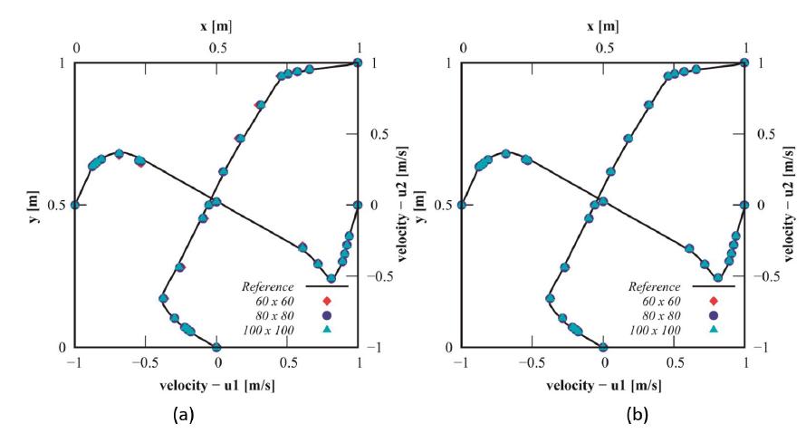
The influence of the refinement level over the present numerical predictions is initially analyzed using three control mesh configurations (60x60, 80x80 and 100x100) with basis functions degree defined by p = q = 1 and refinement parameters h = 0.001L and h = 0.0025L. The flow is characterized with a Reynolds number Re = 10³. Notice that these mesh configurations reproduce classical finite element grids with Lagrangian basis functions and C ⁰-continuity order. Figure 5 shows velocity profiles along the horizontal and vertical lines of the cavity referring to results obtained here and the corresponding predictions obtained by Ghia et al. (1982), who adopted a second-order finite difference model with 257x257 grid points.

One can see that a very good agreement is obtained with respect to the reference predictions by using h = 0.0025L and any of the mesh configurations proposed in the present application. On the other hand, when a mesh parameter h = 0.001L is adopted, differences are observed in the central region of the cavity, where predictions are improved as the number of control points of the mesh configuration is increased. Nevertheless, a very good agreement is also obtained near the wall regions for all mesh configurations utilized here. One can notice that excessive refinement near the wall regions (h = 0.001L) may lead to insufficient refinement in the central region of the cavity when coarse meshes are utilized.

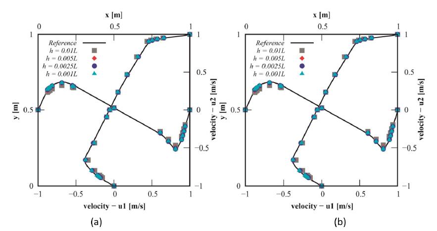
In order to analyze the influence of mesh parameter h in the present study, two control mesh configurations (80x80 and 100x100) are adopted using basis functions with p = q = 1. Results referring to velocity profiles along the horizontal and vertical centerlines of the cavity are presented in Figure 6, where results obtained here are compared with numerical predictions obtained by Ghia et al. (1982) for Re = 10³.

The effect of mesh parameter h over the numerical predictions is clearly demonstrated. It is observed that insufficient results are obtained when h = 0.01L is adopted, independent of the mesh configuration utilized. One can also notice that the effect of using a more refined mesh configuration over the numerical results is small in this case.

The influence of basis functions over the numerical results is investigated here using an intermediate control mesh configuration (80x80) and two intermediate refinement parameters, h = 0.0025L and h = 0.005L. The present results are shown in Figure 7, which are compared with predictions obtained by Ghia et al. (1982).

Figure 5
Influence of control mesh configuration: velocity profiles along the horizontal and vertical centerlines of the cavity for Re = 10³; basis functions: p = q = 1; refinement parameter: (a) h = 0.001L, (b) h = 0.0025L.

Figure 6
Influence of mesh parameter h: velocity profiles along the horizontal and vertical centerlines of the cavity for Re = 10³; basis functions: p = q = 1; control mesh configuration: (a) 80x80, (b) 100x100.

Figure 7
Influence of basis functions: velocity profiles along the horizontal and vertical centerlines of the cavity for Re = 10³; control mesh configuration: 80x80; mesh parameter: (a) h = 0.0025L, (b) h = 0.005L.

Turbulence is also analyzed in the present application considering a LES-type approach with C_S = 0.15 (see Eq. 6) and flow conditions defined by Re = 10⁴. An intermediate control mesh configuration (100x100) is utilized here with different basis functions (p = q = 1, 2 and 3) and two refinement parameters: h = 0.001L and h = 0.0025L. Results are presented in Figure 8, where comparisons are performed taking into account predictions obtained by Ghia et al. 1982 for Re = 10⁴.

Figure 8
Influence of turbulence: velocity profiles along the horizontal and vertical centerlines of the cavity for Re = 10⁴; control mesh configuration: 100x100; mesh parameter: (a) h = 0.001L, (b) h = 0.0025L.

The present results demonstrate that the control mesh configuration with mesh parameter h = 0.001L is clearly insufficient to reproduce the reference results, independent of the basis function degree utilized. In this sense, one can observe that by increasing the basis function degree, accuracy is gradually reduced, especially in the central region of the cavity. On the other hand, when the mesh parameter h value is increased to h = 0.0025L, the present results are improved. In addition, the influence of the basis function degree is now inverted, leading to better predictions when the function degree is increased, although the improvements are not significant in this case. Excessive refinement near the wall regions led again to insufficient refinement in the central region of the cavity when a coarse mesh was utilized.

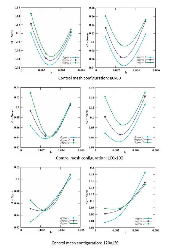
An overall evaluation of the present results can be performed considering Figures 9 and 10, where mesh quality is determined using the Euclidean norm of vectors of velocity variation. These vectors are defined taking into account sample points proposed by Ghia et al. (1982) to define the velocity profiles along the center lines of the cavity (see Ghia et al. (1982) for detailed information). The Euclidean norms referring to velocity vector components are defined here as follows:

$v_1^{h_j}-norm=\sqrt{{\displaystyle \sum _{i=1}^n{\left[{\left(v_1^{h_{j+1}}\right)}_i-{\left(v_1^{h_j}\right)}_i\right]}^2}};v_2^{h_j}-norm=\sqrt{{\displaystyle \sum _{i=1}^n{\left[{\left(v_2^{h_{j+1}}\right)}_i-{\left(v_2^{h_j}\right)}_i\right]}^2}}$ (70)

where v ₁ and v ₂ are velocity vectors obtained from sample points located on the center lines of the cavity according to positions defined by Ghia et al. 1982 and n is the number of sample points. Notice that each velocity vector corresponds to a specific refinement parameter h_j (j = 1,…,4), with h₁ = 0.001L, h₂ = 0.0025L, h₃ = 0.005L, h₄ = 0.01L.

It is observed that mesh configurations with an insufficient number of control points lead to inaccurate predictions, where the use of smaller mesh parameters h and basis functions with higher degree deteriorates the numerical results due to inadequate spatial discretization. This effect may also be associated with the refinement procedure proposed for the present application, where the control points were distributed arbitrarily. For a control mesh configuration with an appropriate number of control points, mesh parameter and basis function degree, one can notice that v ₁ and v ₂ norms behave asymptotically with respect to mesh parameter h, converging usually to a determined error level as h → 0, which may also be null if the spatial discretization is optimized. In addition, basis functions with low continuity order lead to slightly better results when the present refinement procedure is adopted.

Figure 9
Euclidean norms: $v_1^{h_j}-norm$ and $v_2^{h_j}-norm$ as functions of the refinement parameter h_j. Reynolds number: Re = 10³.

Figure 10
Euclidean norms: $v_1^{h_j}-norm$ and $v_2^{h_j}-norm$ as functions of the refinement parameter h_j. Reynolds number: Re = 10⁴.

The same effects formerly reported with respect to numerical predictions obtained with insufficient mesh configurations are observed here and amplified. Considering that a flow with higher Reynolds number is simulated, higher levels of spatial discretization are required. The asymptotic behavior of v ₁ and v ₂ norms as functions of the mesh parameter h is only identified for the control mesh configuration 120x120. Results indicate that the mesh configurations utilized in this case are not sufficiently optimized. This aspect may be associated with the spatial discretization methodology proposed in this work, where the control points are arbitrarily distributed over the computational domain. For a high Reynolds number flow, basis functions with higher degrees seem to lead to better results when compared with predictions obtained with low-order basis functions, which are traditionally adopted by lagrangian-based finite element formulations.

The cavity flow field is shown in Figure 11, where pressure field and streamlines obtained with the present formulation are presented. One can notice that the present predictions agree very well with the classic results obtained by Ghia et al. (1982), with primary, secondary and tertiary recirculation zones reproduced correctly according to the Reynolds number adopted.

Figure 11
Pressure field and streamlines.

4.2 Flow around circular cylinder

The flow around circular cylinder is analyzed here using a wide range of Reynolds numbers and different refinement procedures, where a viscous fluid under incompressible flow regime is utilized. Although it is well known that the flow regime around circular cylinders is turbulent for Re > 300 (see, for instance, Lienhard, 1966), a two-dimensional approach is adopted here as a first approximation to the actual problem. NURBS basis functions are adopted for spatial discretization.

The numerical model is initially validated using a computational domain constituted by a single patch and quadratic basis functions in both parametric directions (p = q = 2), where uniform knot vectors are employed. It is important to notice that quadratic NURBS functions must be employed along the angular direction (p), at least, in order to obtain a circular curve exactly (see Piegl and Tiller, 1997). The flow field is characterized using inflow velocity v_∞= 10 m/s and the following Reynolds numbers (Re): 10, 20, 30, 40, 50, 100, 300, 500, 700 and 1000, where control mesh configurations of 100x70, 120x90 and 168x120 control points are employed for 10 ≤ Re ≤ 50, 100 ≤ Re ≤ 300 and 500 ≤ Re ≤ 1000, respectively. Control points are distributed along the radial direction using geometric progression, considering that the smaller distance between two consecutive control points corresponds to the first pair of control points next to the cylinder surface. This smaller value is defined here as the mean distance between consecutive control points along the angular direction, which are only related to control points associated with the cylinder surface. The time increment Δt is obtained using Eq. (57) with α = 0.3. Computational domain and boundary conditions utilized in the present analysis are shown in Figure 12.

Figure 12
Flow on circular cylinder: computational domain referring to single patch analysis.

Results referring to drag coefficient (C_D) and Strouhal number (St) are presented in Table 2, where predictions obtained in this work are compared with results obtained numerically by Henderson (1997). Drag (C_D) and lift (C_L) coefficients, as well as the Strouhal number (St), are obtained here using the following expressions:

$C_D=\frac{{\displaystyle \sum _{e=1}^{nel}\left(-{\displaystyle \underset{{\Gamma }_e}{\int }{t}_1^f}d\Gamma \right)}}{\frac{1}{2}\rho V^{2}D};C_L=\frac{{\displaystyle \sum _{e=1}^{nel}\left(-{\displaystyle \underset{{\Gamma }_e}{\int }{t}_2^f}d\Gamma \right)}}{\frac{1}{2}\rho V^{2}D};St=\frac{fD}{V}$ (71)

where V is the undisturbed flow speed, D is the cylinder diameter, f is the vortex shedding frequency obtained from time histories of lift coefficient, $t_1^f$ and $t_2^f$ are the horizontal and vertical components of the fluid traction vector t ^f, which is evaluated using Eq. (10) for a point located at the fluid-structure interface, Γ_e is the boundary of element e in contact with the cylinder surface and nel is the number of fluid elements on the cylinder surface. An excellent agreement with the reference results can be observed.

Table 2
Flow on circular cylinder: drag coefficient (C_D) and Strouhal number (St) for 10 ≤ Re ≤ 1000.

Reynolds number (Re)	Present work		Henderson 1997
	CD	St	CD	St
10	2.929	-	2.789	-
20	2.108	-	2.064	-
30	1.769	-	1.730	-
40	1.583	-	1.546	-
50	1.450	-	1.449	-
100	1.370	0.165	1.360	0.167
300	1.360	0.205	1.379	0.211
500	1.417	0.225	1.430	0.225
700	1.434	0.232	1.483	0.231
1000	1.491	0.234	1.502	0.237

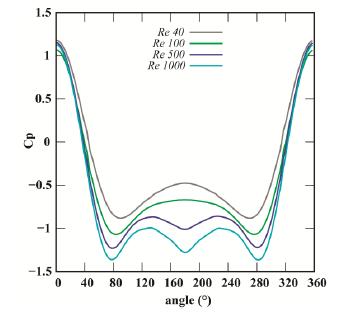
Flow characteristics may be observed in Figure 13, where streamlines and pressure fields are presented. One can notice that a recirculation zone is formed behind the cylinder for Re = 10, 20 and 30, while the von Karman vortex street with alternate vortex shedding is obtained for Re = 100, 500 and 1000, which demonstrates that the formulation proposed in this work can reproduce complex flow phenomena accurately. The distribution of pressure coefficient over the cylinder perimeter is shown in Figure 14 for some of the Reynolds numbers investigated here.

Figure 13
Flow around circular cylinder: pressure field and streamlines for different Reynolds numbers.

Figure 14
Distribution of pressure coefficient over the cylinder perimeter for different Reynolds numbers.

The influence of the basis functions on the present results is evaluated using a control mesh configuration with 100x70 control points and flow conditions defined by Re = 40. Two basis function configurations are compared: (a) quadratic functions in both parametric directions (p = q = 2) and (b) quadratic functions in the angular direction (p = 2) with linear functions in the radial direction (q = 1).

Figure 15
Flow around circular cylinder at Re = 40: geometric aspects.

Table 3
Drag coefficient (CD) and geometric characteristics of the recirculation zone behind the circular cylinder for Re = 40.

Parameter	Mesh 1 (p = q = 2)	Mesh 2 (p = 2; q = 1)	Reference
CD	1.58	1.62	1.60
L/D	2.21	2.23	2.10
a/D	0.71	0.71	0.69
b/D	0.59	0.59	0.58
θ [deg]	52.10	51.50	53.20

Results referring to drag coefficient (C_D) and geometric characteristics of the recirculation zone obtained behind the circular cylinder are summarized in Table 3, which are defined considering the geometric parameters presented in Figure 15. The present results are compared with numerical predictions obtained by Wanderley and Levi (2002) using a finite difference model, where a good agreement is obtained using both the basis functions proposed here, although results obtained with p = q = 2 are slightly better. It is important to notice that a mesh configuration with p = 2 and q = 1 lead to significant reductions in terms of computational efforts when compared with the processing time spent by the mesh configuration with p = q = 2, considering that full Gauss quadrature is employed here for numerical evaluation of finite element quantities, such as element matrices and vectors.

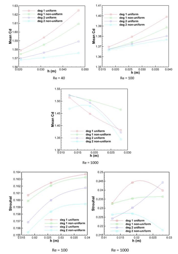
Additional simulations are performed in order to evaluate the influence of refinement parameter h (smallest distance between adjacent control points), uniformity of the knot vectors and basis degree over the numerical results. For Re = 40, three refinement levels are utilized, which are defined by h = 2.09x10^-2 m, h = 3.14x10^-2 m and h = 4.71x10^-2 m. For Re = 100, the following refinement parameters are considered: h = 1.75x10^-2 m, h = 2.62x10^-2 m and h = 3.93x10^-2 m. Finally, h = 1.25x10^-2 m, h = 1.87x10^-2 m and h = 2.80x10^-2 m are utilized for Re = 1000. Configurations with linear and quadratic basis functions in both parametric directions are also considered.

Results obtained with the present formulation are shown in Figure 16, where drag coefficient and the Strouhal number are considered. It is observed that spatial discretizations with non-uniform knot vectors generally lead to better convergence when compared with predictions obtained using uniform knot vectors. In addition, degree elevation also improved convergence for flow conditions defined by Re = 40 and Re = 100. However, one can notice that similar trends are not observed for Re = 1000.

Figure 16
Flow around circular cylinder: drag coefficient and Strouhal number.

4.3 Backward-facing step flow

The backward-facing step flow is investigated in the present example using multi-patch refinement, where the computational domain is decomposed into parametrically independent sub-domains. This procedure is useful for applications with complex geometry or complex flow fields. Six different flow conditions are analyzed, which are characterized by the following Reynolds numbers: Re = 100, 200, 400, 600, 800 and 1000.

Five patches are utilized here, where mesh control configurations were defined considering a uniform distribution of control points and different combinations of basis function degrees along the respective parametric direction (p = q = 1; p = q = 2; p = 1 and q = 2 for patches 1 and 4 only, with p = q = 1 for the remaining patches). The control points are distributed over the patches as follows:

• for Re = 100: patches 1 and 4 - 60x20, patches 2 and 3 - 200x20 and patch 5 - 20x20;

• for Re = 200: patches 1 and 4 - 100x20, patches 2 and 3 - 180x20 and patch 5 - 20x20;

• for Re = 400: patches 1 and 4 - 200x24, patches 2 and 3 - 220x24 and patch 5 - 24x24;

• for Re = 600: patches 1 and 4 - 274x24, patches 2 and 3 - 200x24 and patch 5 - 24x24;

• for Re = 800 and 1000: patches 1 and 4 - 400x30, patches 2 and 3 - 224x30 and patch 5 - 30x30;

The computational domain utilized in the present investigation is shown in Figure 17, where the patch distribution is identified. The geometric characteristics of the channel are defined as follows: h = 1m, s = 0.94 m, x_e = 1m, x_t = 30 m, L₁ = 1 m, L₂ = 17 m and L₃ = 12 m. No-slip boundary conditions are adopted on the channel walls, while a velocity profile with parabolic distribution is prescribed at the channel entrance. The outflow condition is imposed considering p = 0 at the channel exit. The parabolic inflow velocity is defined using:

$v_1\left(x_2\right)=V_1^{\max }\left\{1-{\left[\frac{\left(x_2-s\right)-h/2}{h/2}\right]}^2\right\}$ (72)

where $V_1^{\max }$ is the maximum velocity (10 m/s) over the velocity profile and x₂ is the vertical coordinate defined with respect to the coordinate system shown in Figure 17. The Reynolds number is calculated according to the expression presented in Armaly et al. (1983):

$\mathrm{Re}=\frac{\rho \left(\frac{2}{3}{V}_1^{\max }\right)2h}{\mu }$ (73)

Figure 17
Backward-facing step flow: computational domain.

Results obtained with the numerical model proposed in this work are presented in Table 4, where predictions referring to reattachment length in the recirculation region after the facing step are compared with experimental results obtained by Armaly et al. (1983) and numerical results obtained by Williams and Baker (1997) with a two-dimensional finite element model. The reattachment length is normalized with respect to the geometric parameter s (see Figure 17). One can observe that the reattachment lengths obtained here for Reynolds < 400 are close to experimental results obtained by Armaly et al. (1983), while a better agreement is obtained with respect to numerical predictions obtained by Williams and Baker (1997) for Re ≥ 400. It is important to notice that two-dimensional numerical models underestimate the extent of the primary separation region for Reynolds numbers greater than 400 when compared with predictions obtained experimentally. It has been postulated that this disagreement between physical and computational experiments is due to the onset of three-dimensional flow near Re = 400 (Williams and Baker, 1997).

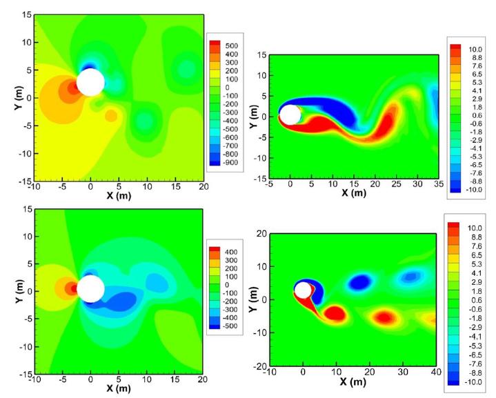
Figure 18 shows streamlines obtained numerically for the flow region after the backward facing step. One can notice that the reattachment length increases as the Reynolds number is increased. In addition, it is observed that a secondary recirculation region is formed along the superior wall of the channel for Re ≥ 600. These observations are in agreement with results presented by Williams and Baker (1997).

Table 4
Backward-facing step flow: normalized reattachment length Xr/s.

	Xr/s
	100	200	400	600	800	1000
Present work (p = q = 1)	2.82	4.82	7.96	9.60	10.59	11.65
Present work (p = q = 2)	2.83	4.84	7.98	9.60	10.61	11.65
Present work (p = 1, q = 2, patches 1 and 4 only)	2.79	4.74	7.91	9.50	10.37	11.49
Armaly et al. (1983) - exp	3.07	5.19	8.74	11.54	14.26	16.32
Williams and Baker (1997) - num 2D	2.42	4.40	8.10	-	10	-

Figure 18
Backward-facing step flow: streamlines as functions of the Reynolds number.

Flow conditions can also be evaluated using the pressure fields obtained here as functions of the Reynolds number, which are presented in Figure 19. For Re = 600, 800 and 1000, these flow fields are obtained considering a time average over the last half of the simulation period. Taking into account that patch interfaces are critical for the present formulation, where basis functions are only C ⁰-continuous, it is observed that streamlines (Figure 18) and pressure isolines are well defined near the patch interfaces, where oscillations are not identified.

Figure 19
Backward-facing step flow: pressure fields as functions of the Reynolds number.

4.4 Lock-in analysis for elastically supported circular cylinder

In the present example, the lock-in phenomenon observed in elastically-mounted circular cylinders submitted to fluid flow is numerically simulated. It is well known that the lock-in phenomenon occurs for a specific range of flow speeds, where synchronization between the mechanical frequency of the structure and the vortex-shedding frequency is obtained. During the lock-in, the amplitude of oscillations is increased, although rarely exceeding half of the cylinder diameter (see, for instance, Simiu and Scanlan, 1996). One can notice that the synchronization frequency is not necessarily the natural frequency of the structure.

The computational domain utilized here is the same as that presented in Figure 12, which is discretized now using a control mesh with 180x120 control points and non-uniform knot vectors. Quadratic NURBS basis functions are adopted in both parametric directions (p = q = 2). This control mesh configuration is obtained from a coarse grid, which is improved by using knot refinement. The grid spacing is gradually reduced towards the cylinder surface, where the smallest distance is Δx = 8.73x10^-2 m. The time step employed in the time integration of the flow equations is Δt = 3.23x10^-2 s (see Eq. 57).

The lock-in phenomenon is investigated using a fixed Reynolds number Re = 150 and different reduced velocities (V_red = V/f.D) within the range 3 ≤ V_red ≤ 8. The cylinder is restricted in angular and horizontal directions and free to vibrate perpendicularly to the flow, which is mechanically described with the following dimensionless form of the structure equation of motion:

$\frac{{\partial }^2{u}_y}{\partial t^2}+\frac{4\pi \xi }{V_{red}}\frac{\partial u_y}{\partial t}+\frac{4{\pi }^2}{V_{red}^2}{u}_y=\frac{1}{2M_{red}}{C}_y$ (74)

where u_y and C_y are the structure displacement and force coefficient transverse to the flow direction, ξ is the damping ratio and M_red = M/ρD² is the reduced mass. In the present investigation, no damping is considered and a constant reduced mass M_red = 2 is adopted.

The structural response obtained with the present formulation is shown in Figure 20 for some of the reduced velocities analyzed here. The typical lock-in response can be clearly identified for V_red = 4, while a structural response with relatively low displacement amplitudes are observed when V_red = 8 is considered. In Figure 21, the normalized maximum displacement of the structure is plotted against reduced velocity and compared with other numerical predictions (Ahn and Kallinderis, 2006; Borazjani et al., 2008), where one can see that the lock-in interval can be identified within the reduced velocity range 4 ≤ V_red ≤ 7, considering that the vibration amplitude is significantly reduced outside this range.

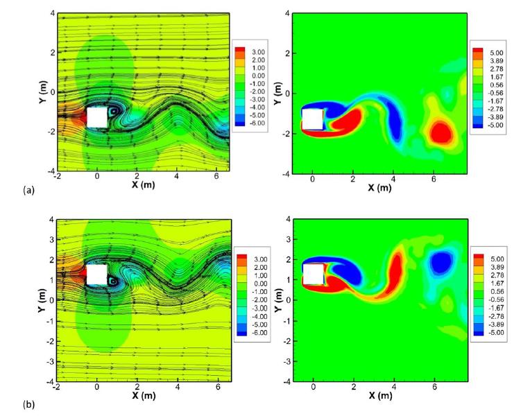
The flow field may be evaluated using Figure 22, where instantaneous pressure and vorticity are presented for V_red = 4 and V_red = 8 at t = 80 s. These results are similar to predictions obtained numerically by Borazjani et al. (2008) using a FSI model and the immersed boundary method.

Figure 20
Lock-in analysis: structural response for different reduced velocities.

Figure 21
Lock-in analysis: normalized maximum displacement as a function of the reduced velocity.

Figure 22
Lock-in analysis. Instantaneous pressure and vorticity obtained at t = 80s: a) V_red = 4; b) V_red = 8.

4.5 Galloping analysis of an elastically supported square cylinder

Galloping is numerically simulated here considering a square cylinder with an elastic support mounted transverse to the flow direction. The galloping phenomenon is typically found in structures with special cross-section shapes, such as rectangular ad D shapes, which may exhibit large amplitude oscillations in the direction normal to the flow at lower frequencies than those associated with vortex shedding (see Simiu and Scanlan, 1996).

Geometry and boundary conditions utilized in the present application are found in Figure 23, where dimensionless values are indicated. The computational domain is discretized using 180x90 control points, non-uniform knot vectors with linear basis functions in the angular direction and quadratic basis functions in the radial direction. The smallest grid distance is found next to the cylinder surface with Δx* = 2.22 x10^-2 and the time step for time integration is set to Δt* = 1.26 x10^-4. The structure properties are presented in dimensionless form as follows: m* = 20, c* = 0.0581195 and k* = 3.08425. The fluid flow is characterized by a Reynolds number Re = 250, where the dimensionless fluid parameters are defined as: v*∞ = 2.5, ρ* = 1.0 and μ* = 0.01. Notice that asterisks indicate dimensionless values.

Figure 23
Galloping analysis: computational domain and boundary conditions.

The structural response obtained here is presented in Figure 24 and instantaneous flow conditions are shown in Figure 25, where the pressure and vorticity fields are presented at t* = 301.93 and t* = 310.61. One can observe that the displacement amplitude is relatively large and limited, which characterizes the typical conditions for dynamic instability by Galloping. Table 5 summarizes the present results referring to maximum displacement amplitude and frequency of oscillation, which are compared with predictions obtained from other authors (Dettmer and Peric, 2006; Robertson et al., 2003). Results obtained here demonstrate a very good agreement with other predictions considering flow aspects and structural vibration characteristics.

Figure 24
Galloping analysis: structural response, vertical displacement.

Table 5
Galloping analysis: maximum displacement and frequency of oscillation.

	Max. displacement	Frequency of oscillation
Present work	1.25	0.945 fn
Dettmer and Peric (2006)	1.117	0.943 fn
Robertson et al. (2003)	1.150	0.938 fn

Figure 25
Galloping analysis: pressure and vorticity fields at (a) t = 301.93s and (b) t = 310.61s.

4.6 Flow over elastically supported rectangular cylinder

Fluid-rigid body interaction is analyzed in this example considering a rectangular cylinder immersed in a viscous fluid flow. Two conditions are investigated: (a) the structure is released from an initial angular displacement with the fluid at rest and no structural damping; (b) the structure is submitted to uniform flow, where vertical and angular displacements are induced simultaneously. The computational domains and boundary conditions adopted in the present analyses are shown in Figure 26.

Figure 26
Flow over rectangular cylinder: computational domain and boundary conditions.

In the first investigation, the cylinder is released from an initial angular displacement of θ₀ = 5°, considering that fluid and structure are at rest. The structural properties are defined taking into account a torsional frequency $\omega =\sqrt{k_{\theta }/I}=0.266rad/s$, where k_θ is the torsional stiffness, and I is the mass moment of inertia. No structural damping is considered in the present analysis and three Reynolds numbers are utilized. The Reynolds number associated with the flow is calculated here using a characteristic length L = b/2 = 1.25 m, where b is the base of the rectangle, and a characteristic flow speed $V=\omega {\theta }_0\sin \left(\omega T/2\right)L=2.90245x{10}^{-2}m/s$, where T is the period of vibration. A control mesh with 161x71 control points is utilized, which is obtained considering knot refinement from an initial coarse mesh. Uniform knot vector in the angular direction and non-uniform knot vector in the radial direction are adopted, considering that linear basis functions are employed in both parametric directions.

Results referring to the structural response obtained with the present formulation are shown in Figure 27. One can observe that the angular displacements are gradually reduced over the time due to the action of fluid viscosity since no structural damping is considered here. In addition, notice that flow damping gets more significant as the Reynolds number is reduced. The present predictions are in agreement with results presented by Sarrate et al. (2001), where a finite element model was utilized.

Figure 27
Flow over rectangular cylinder: structural response with fluid at rest

In the second investigation proposed here, the rectangular cylinder is analyzed considering the action of a uniform flow (see Figure 26), which leads to vertical and angular displacements in the structure. The dimensionless parameters referring to the structure properties are set as follows: m_t = 195.57, c_t = 0.0325, k_t = 0.7864, I = 105.94, c_r = 0.0 and k_r= 17.05, where m, I, c and k denote mass, mass moment of inertia, damping and stiffness constants and the subscripts t and r are related to translational and rotational degrees of freedom. The flow field is characterized by a Reynolds number Re = 1000.

A control mesh configuration with 161x71 control points is employed, which is similar to that utilized in the previous study. Comparisons are performed considering mesh configurations with uniform and non-uniform knot vectors. In addition, predictions obtained from a mesh configuration with linear basis functions in both parametric directions are compared with results obtained from a mesh with linear basis functions in the angular direction and quadratic basis functions along the radial direction.

Figure 28
Flow over rectangular cylinder: structural response under uniform flow.

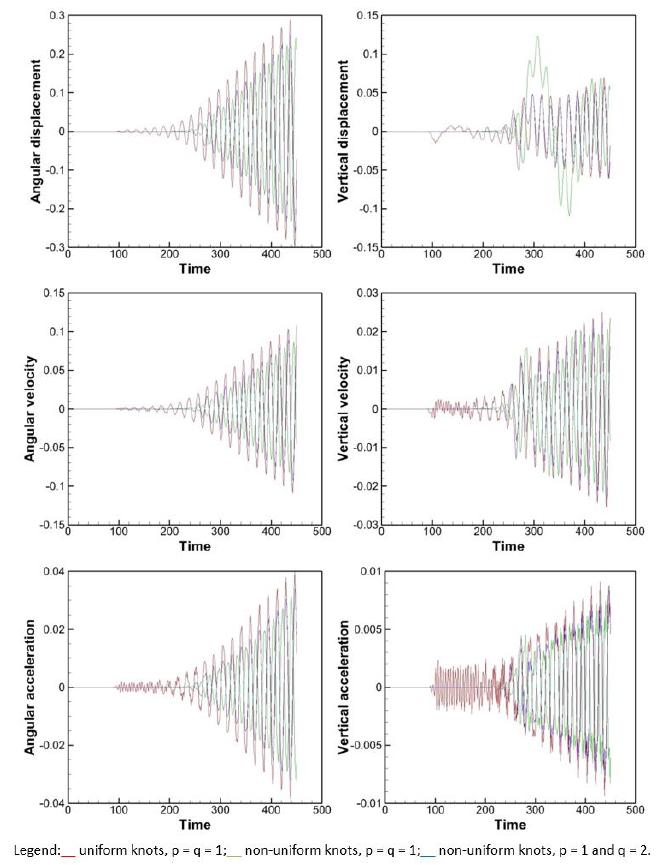
The structural responses obtained here are presented in Figure 28, where predictions referring to different mesh conditions are compared. Notice that the structural vibration is anticipated when uniform knot vectors are adopted, although the increase rate and oscillation frequency are the same as those obtained with non-uniform knot vectors. The use of basis with a higher degree also anticipates the onset of structural vibration without modifying the increase rate and frequency of oscillation. When linear basis are utilized in conjunction with non-uniform knot vectors, vertical displacements with greater amplitude are obtained in the early stages of the structural response.

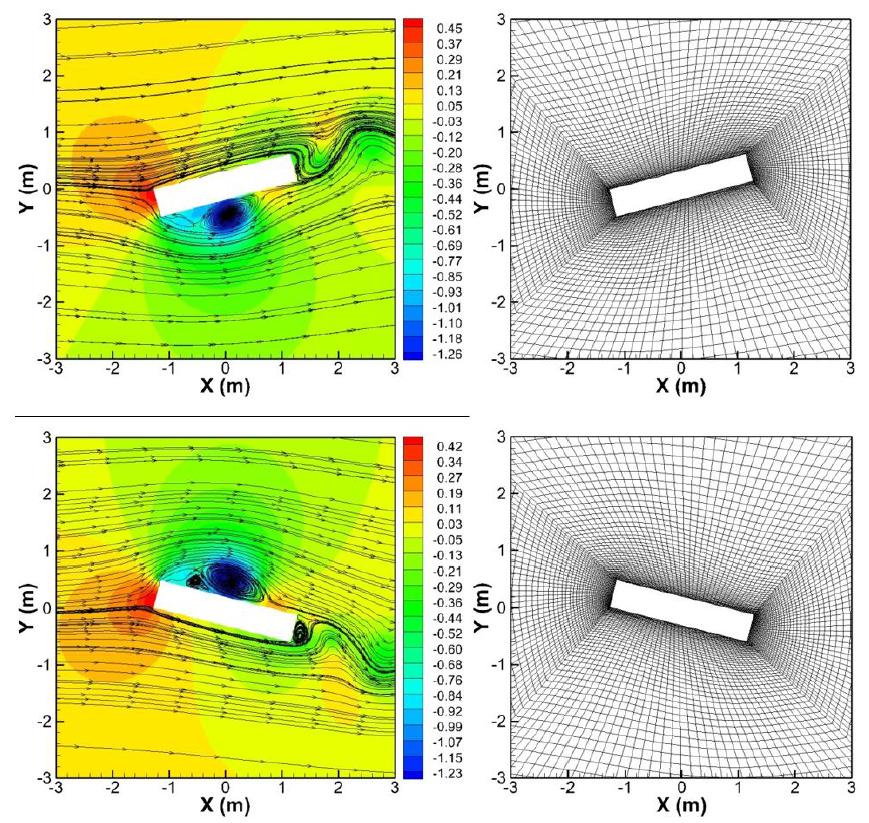
The mesh configuration and the corresponding pressure field and streamlines for dimensionless time instants t* = 439 and t* = 448 are shown in Figure 29, where one can see that the mesh motion scheme adopted in the present work can accommodate the structural motion in the region next to the immersed body without excessive distortion. It is important to notice that using n = 4 in Eq. 20, one obtains a mesh motion such that elements near the immersed body show motion characteristics similar to rigid bodies, maintaining its original geometric aspects. On the other hand, elements located in the intermediate region between the fluid-structure interface and the outer border of the ALE domain present deformation similar to elastic bodies. As exponent n is reduced, this elastic aspect of the element motion is observed in the mesh region near the immersed body.

Figure 29
Flow over rectangular cylinder: mesh configuration, pressure field and streamlines at t* = 439 and t* = 448.

5 CONCLUSIONS

In the present work a NURBS-based finite element formulation for incompressible fluid dynamics and fluid-structure interaction with rigid-body dynamics was presented. Model versatility with respect to spatial discretization procedures was demonstrated, where different techniques referring to NURBS discretization, such as multi-patches, knot insertion, and degree elevation, were adopted. In addition, a control mesh discretization scheme was proposed, where control point locations are specified arbitrarily. The present investigation indicates that results obtained with the present model are very sensitive to the mesh configuration utilized. In this sense, if the control mesh distribution is not adequately set, good predictions are not obtained even with high degree basis functions. In this case, the use of functions with higher degree leads to deterioration of the numerical predictions. On the other hand, one can observe that improvements can be obtained by using higher degree basis functions when flows with high Reynolds numbers are investigated, especially for turbulent flows. The use of non-uniform knot vectors usually leads to better results when compared with predictions obtained with uniform knot vectors. This aspect is important in order to capture complex flow phenomena, especially in the boundary layer region. Computational efforts are usually high when the present formulation is applied to turbulent flows, considering that full Gauss quadrature is employed in this work to evaluate element matrices and vector. This drawback may be circumvented by using specialized techniques for numerical integration of NURBS basis functions. In this sense, a reduced integration formulation for NURBS-based finite element models may also be developed. For future works, the present formulation must be extended to include the three-dimensional approach. Potential applications for the present model may be found in the field of Computational Wind Engineering, such as aerodynamic and aeroelastic analyses of long-span bridges, low and high-rise buildings.

Acknowledgments

The authors would like to thank CNPq and CAPES for the financial support, and CESUP-UFRGS and CENAPAD-UNICAMP for technical support and computational resources provided.

References

• Ahn H. T., Kallinderis Y., (2006). Strongly coupled flow/structure interactions with a geometrically conservative ALE scheme on general hybrid meshes. Journal of Computational Physics 219:671-696.
• Akkerman I., Bazilevs Y., Kees C. E., Farthing M. W., (2011). Isogeometric analysis of free-surface flow. Journal of Computational Physics 230: 4137-4152.
• Armaly B. F., Durst F. J., Pereira C. F., Schönung B., (1983). Experimental and theoretical investigations of backward-facing step flow. Journal of Fluid Mechanics 127: 473-496.
• Bathe J., (1996). Finite Element Procedures, 1st Edition. Prentice Hall, Englewood Cliffs-NJ, USA.
• Bazilevs Y., Calo V. M., Zhang Y., Hughes T. J. R., (2006). Isogeometric fluid-structure interaction analysis with applications to arterial flow. Computational Mechanics 38: 310-322.
• Bezier P., (1972). Numerical Control: Mathematics and Applications. Wiley, London.
• Borazjani I., Ge L., Sotiropoulos F., (2008). Curvilinear immersed boundary method for simulating fluid structure interaction with complex 3D rigid bodies. Journal of Computational Physics 227: 7587-7620.
• Braun A. L., Awruch A. M., (2009). Aerodynamic and aeroelastic analyses on the CAARC standard tall building model using numerical simulation. Computers and Structures 87: 564-581.
• Chorin A. J., (1967). A numerical method for solving incompressible viscous flow problems. Journal of Computational Physics, 2: 12-26.
• Cottrell J. A., Hughes T. J. R., Bazilevs Y., (2009). Isogeometric Analysis: Toward Integration of CAD and FEA, John Wiley & Sons, 2009.
• Cox M. G., (1972). Numerical evaluation of B-splines. Journal of the Institute of Mathematics and its Applications, 10: 134-149.
• De Boor C., (1972). On calculation with B-splines. Journal of Approximation Theory 6: 50-62.
• Dettmer W. G., Peric D., (2006). A computational framework for fluid-rigid body interaction: Finite element formulation and applications. Computers Methods in Applied Mechanics and Engineering 195: 1633-1666.
• Espath L. F. R., Braun A. L., Awruch A. M., Dalcin L. D., (2015). A NURBS-based finite element model applied to geometrically nonlinear elastodynamics using a corotational approach. International Journal for Numerical Methods in Engineering 102: 1839-1868.
• Espath L. F. R., Braun A. L., Awruch A. M., Maghous S., (2014). NURBS-based three-dimensional analysis of geometrically nonlinear elastic structures. European Journal of Mechanics-A/Solids 47: 373-390.
• Ghia U., Ghia K. N., Shin C. T., (1982). High-Re solutions for incompressible flow using the Navier-Stokes equations and multigrid method. Journal of Computational Physics 48: 378-411.
• Gomez H., Calo V. M., Bazilevs Y., Hughes T. J. R., (2008). Isogeometric analysis of the Cahn-Hilliard phase-field model. Computer methods in applied mechanics and engineering 197: 4333-4352.
• Gomez H., Hughes T. J. R., Nogueira X., Calo V. M., (2010). Isogeometric analysis of the isothermal Navier-Stokes-Korteweg equations. Computer Methods in Applied Mechanics and Engineering 199: 1828-1840.
• Henderson R., (1997). Nonlinear dynamics and pattern formation in turbulent wake transition. Journal of Fluid Mechanics 352: 65-112.
• Kadapa C., Dettmer W. G., Peric D., (2015). NURBS based least-squares finite element methods for fluid and solid mechanics. International Journal for Numerical Methods in Engineering 101: 521-539.
• Kawahara M., Hirano H., (1983). A finite element method for high Reynolds number viscous fluid flow using two step explicit scheme. International Journal for Numerical Methods in Fluids 3: 137-163.
• Lesoinne M., Farhat C., (1996). Geometric conservation law for flow problems with moving boundaries and deformable meshes, and their impact on aeroelastic computations. Computer Methods in Applied Mechanics and Engineering 134: 70-90.
• Lesoinne M., Farhat C., (1998). Improved staggered algorithms for the serial and parallel solution of three-dimensional nonlinear transient aeroelastic problems. In: Computational Mechanics. S Idelsohn, E Oñate and E Dvorakin (Eds.), Barcelona, CIMNE.
• Lienhard J. H., (1966). Synopsis of Lift, Drag and Vortex Frequency Data for Rigid Circular Cylinders. Washington State University, College of Engineering, Research Division Bulletin 300.
• Nielsen P. N., Gersborg A. R., Gravesen J., Pedersen N. L., (2011). Discretizations in isogeometric analysis of Navier-Stokes flow. Computer methods in applied mechanics and engineering 200: 3242-3253.
• Piegl L., Tiller W., (1997). The NURBS Book, 2nd Edition. Springer-Verlag, Berlin Heidelberg.
• Reddy J. N., Gartling D. K., (2010). The Finite Element Method in Heat Transfer and Fluid Dynamics, 3rd Edition. CRC Press, Boca Raton, USA.
• Robertson I., Sherwin S. J., Bearman P. W., (2003). A numerical study of rotational and transverse galloping rectangular bodies. Journal of Fluids and Structures 17: 681-699.
• Sarrate J., Huerta A., Donea J., (2001). Arbitrary Lagrangian-Eulerian formulation for fluid-rigid body interaction. Computer Methods in Applied Mechanics and Engineering 190: 3171-3188.
• Schoenberg I. J., (1946). Contributions to the problem of approximation of equidistant data by analytic functions. Quarterly of Applied Mathematics 4: 45-99.
• Sederberg T. N., Zhengs J. M., Bakenov A., Nasri A., (2003). T-splines and T-NURCCSs. ACM Transactions on Graphics 22: 477-484.
• Simiu E., Scanlan R. H., (1996). Wind Effects on Structures: Fundamentals and Applications to Design, 3rd Edition. John Willey and Sons, New York, USA.
• Smagorinsky J., (1963). General circulation experiments with the primitive equations, I. the basic experiment. Monthly Weather Review 91: 99-164.
• Townsend A., (2014). On the spline: a brief history of the computational curve. International Journal of Interior Architecture - Spatial Design: Applied Geometries, vol. 3.
• Thomas P. D., Lombard C. K., (1979). Geometric conservation law and its application to flow computations on moving grids. AIAA Journal 17: 1030-1037.
• Wanderley L. B. V., Levi C. A., (2002). Validation of a finite difference method for the simulation of vortex-induced vibrations on a circular cylinder. Ocean Engineering 29: 445-460.
• White F. M., (2005). Viscous Fluid Flow, 3rd Edition. Mc Graw-Hill, New York, USA.
• Williams P. T., Baker A. J., (1997). Numerical simulations of laminar flow over a 3D backward-facing step. International Journal for Numerical Methods in Fluids 24: 1159-1183.
• Zienkiewicz O. C., Taylor R. L., Zhu J. Z., (2013). The Finite Element Method for Fluid Dynamics, 7th Edition. Butterworth-Heinemann, Oxford, UK.

Edited by

Editor:

Marco L. Bittencourt.

Publication Dates

• Publication in this collection
  03 Feb 2020
• Date of issue
  2020

History

• Received
  20 Aug 2019
• Reviewed
  25 Nov 2019
• Accepted
  27 Nov 2019
• Published
  05 Dec 2019