Stability of a half-sine shallow arch under sinusoidal and step loads in thermal environment

Abstract

The complex structural behavior of shallow arches can be remarkably affected by many parameters. In this paper, the structural responses of a half-sine pin-ended shallow arch under sinusoidal and step loadings are accurately calculated. Additionally, the effects of environmental temperature changes are considered. Three types of sinusoidal loadings are separately investigated. Displacements, load-bearing capacity, the magnitude of the axial force and the locus of critical points (including limit and bifurcation points) are directly obtained without tracing the corresponding equilibrium path. Furthermore, the boundaries identifying the number of critical points are investigated. All mentioned structural responses are formulized based on the rise of the arch and the environmental temperature change, which are introduced in a dimensionless form. The proposed formulation is also developed for generalized sinusoidal loadings. Additionally, the structural behavior of the shallow arch under two types of step loadings is investigated. Finally, the accuracy of the suggested approach is examined by a non-linear finite element method.

Keywords
Half-sine shallow arch; equilibrium path; critical point; bifurcation; stability analysis

1 INTRODUCTION

Shallow arches are widely used in structural, mechanical and aerospace engineering, and the investigation of structural stability has always been of the researchers’ interest. The failure of such structures is in the form of material failures, structural instability or a combination of them.

The tendency of structure to return to the static state, after creating a perturbation in the degrees of freedom, is called stability (Thompson and Hunt, 1973; Khalil, 2002). In the analysis of structural stability, since the structure experiences the sudden deformations, the investigation of critical points (such as limit and bifurcation point) is crucial. Such deformations cause severe changes in strains and stresses. The geometry of the arch is an influential parameter on its load-bearing capacity (Cai et al., 2012; Bateni and Eslami, 2015; Bradford et al., 2015; Rezaiee-Pajand and Rajabzadeh-Safaei, 2016). In addition, various loadings (e.g., the sinusoidal (Plaut and Johnson, 1981), concentrated (Pi et al., 2008; Chandra et al., 2012; Tsiatas and Babouskos, 2017), distributed (Moghaddasie and Stanciulescu, 2013b) and end moment loads (Chen and Liao, 2005; Chen and Lin, 2005)), geometric imperfections (Virgin et al., 2014; Zhou et al., 2015a), and boundary conditions (Pi and Bradford, 2012; Pi and Bradford, 2013; Han et al., 2016) are other important factors in the structural design.

In most cases, shallow arches become elastically unstable when the lateral load reaches a critical value (Chen and Li, 2006). This means that a large deformation could be observed while the material remains elastic. Practical experiences also confirm this issue (Chen and Liao, 2005; Chen and Yang, 2007a; Chen and Ro, 2009). Consequently, the behavior of shallow arches can be explained by the non-linear theory of elastic stability. In some analyses, it is assumed that the displacements of the arch are limited to avoid a material failure (Pippard, 1990; Xu et al., 2002; Chen and Hung, 2012). In addition, the variation in the environment temperature can be influential on the stability of structures (Matsunaga, 1996; Hung and Chen, 2012; Stanciulescu et al., 2012; Kiani and Eslami, 2013).

Several approaches can be applied to investigate the structural behavior of shallow arches. Previously, both analytical and numerical methods are discussed in the literature (Plaut and Johnson, 1981; Reddy and Volpi, 1992; Pi et al., 2002; Xenidis et al., 2013). In some analytical techniques, the displacement field is replaced by a set of orthogonal functions to derive the non-linear equilibrium and buckling equations (Xu et al., 2002; Chen et al., 2009; Chen and Hung, 2012; Moghaddasie and Stanciulescu, 2013b; Zhou et al., 2015a). Using the principle of stationary potential energy is another robust analytical approach to investigate the equilibrium and stability of shallow arches (Moon et al., 2007; Pi et al., 2007; Pi et al., 2008; Pi et al., 2010). On the other hand, the non-linear finite element method has been widely applied by researchers to trace the equilibrium path (Chandra et al., 2012; Saffari et al., 2012; Stanciulescu et al., 2012; Zhou et al., 2015b). Identifying the corresponding critical point(s) and finding the relationship between imperfections and load-bearing capacity are the capability of this numerical technique (Eriksson et al., 1999; Moghaddasie and Stanciulescu, 2013b; Rezaiee-Pajand and Moghaddasie, 2014).

This paper provides an analytical method to find the exact response of the half-sine shallow arch under the sinusoidal and step loads. Furthermore, the effect of temperature change on the equilibrium paths is investigated. For this purpose, the displacements of the structure are rewritten in the form of the Fourier series. By the substitution of displacements into the governing equations of the arch, the initial and bifurcated equilibrium path are obtained. On the other hand, the critical (limit and bifurcation) points on the static paths are achieved when the stiffness matrix is singular. In this paper, the behavior of the shallow arch under five types of distributed loads are separately investigated by the suggested approach.

The advantages of the proposed method are: (1) obtaining the exact solution of displacement field, equilibrium paths and the locus of critical points, (2) performing one parametric analysis instead of multiple analyses with specified values, and (3) finding the critical points without tracing the equilibrium paths. On the other hand, some limitations of the supposed method can be listed as (1) the changes in environment temperature are gradual, (2) the theory of plane stress is applied, (3) the height of the arch is limited, and (4) the material remains elastic during the analysis.

In the following section, the governing equations of the half-sine shallow arch under an arbitrary load are provided and the relative equilibrium paths are obtained. Then, the way of finding the locus of critical (limit and bifurcation) points is proposed (Section 3). The behavior of the half-sine arch under a number of distributed loadings is investigated by using the suggested method in Section 4. Finally, concluding remarks are given.

2 THE GOVERNING EQUATIONS OF THE SHALLOW ARCH

In this section, the governing equations of a half-sine shallow arch under an arbitrary loading $Q^{*}$ are obtained (Figure 1(a)). In this regard, a modified Bernoulli beam theory with large transversal displacement is applied. The material is assumed isotropic and variations in the temperature are gradual (no transversal temperature gradient is considered). $E$, $A$, $I$, $\rho$ and ${\alpha }^{*}$, respectively, represent the Young’s modulus, area, moment of inertia, mass density and thermal expansion coefficient, which are assumed to be constant over the span $L$.

Figure 1
A half-sine pinned shallow arch under (a) arbitrary, (b) half-sine, (c) one-sine, (d) one and half-sine, (e) symmetric and (f) asymmetric loadings

The assumptions used for the analysis are as follows: (1) The axial force is constant over the span (Xu et al., 2002; Plaut, 2009; Chen and Hung, 2012); (2) The material is elastic (Chen and Li, 2006); (3) out-of-plane deflections are neglected (Chen and Yang, 2007a); and (4) The range of displacements and curvatures of the arch is small in comparison with the length of the span $(0\le y_{\max }/L<1/10-1/50)$ (Xu et al., 2002). Given the above assumptions, the equation of motion can be written as follows (Plaut and Johnson, 1981; Chen and Yang, 2007b; Chen et al., 2009):

$\rho A{y}_{,tt}=-EI{(y-y_0)}_{,xxxx}+P^{*}{y}_{,xx}-Q^{*}$ (1)

where, $y_0$ is the initial shape of the arch, the subscripts “,$t$” and “,$x$” show the partial differentiation with respect to the time and the longitudinal position of arch, respectively. The value of the axial force ($p^{*}$) is

$P^{*}=EA(-{\alpha }^{*}\Delta T_0+\frac{1}{2L}{\displaystyle {\int }_0^L(y_{,x}^2-y_{\mathrm{0,}x}^2)dx)}$ (2)

Here, $\Delta T_0$ denotes environmental temperature changes.

Since the supports are fixed at the ends, the displacement of the arch in the direction $\text{x}$ is neglected. In addition, the temperature change can cause the axial force in the structure, which is denoted by the term $-EA{\alpha }^{*}\Delta T_0$. Eqs. (1) and (2) could be rewritten in a dimensionless form:

$u_{,\tau \tau }=-{(u-u_0)}_{,\xi \xi \xi \xi }+p{u}_{,\xi \xi }-Q$ (3)

$p=-\alpha \Delta T_0+\frac{1}{2\pi }{\displaystyle \underset{0}{\overset{\pi }{\int }}(u_{,\xi }^2-u_{\mathrm{0,}\xi }^2)d\xi }$ (4)

where,

$\begin{array}{cc}(u,u_0)=\frac{1}{r}(y,y_0),& \begin{array}{cc}\xi =\frac{\pi }{L}x,& \tau =\frac{{\pi }^{2}r}{L^2}\sqrt{\frac{E}{\rho }t},\begin{array}{cc}Q=\frac{L^3}{{\pi }^{3}EIr}Q*,& \alpha =\frac{L^2}{{\pi }^2{r}^2}{\alpha }^{*}\end{array}\end{array}\end{array}$ (5)

Here, $r$ represents the radius of gyration of the cross section calculated by $r=\sqrt{I/A}$. The boundary conditions for Eq. (3) is as follows:

$u(0)-u_0(0)=\mathrm{0,}{u}_{,\xi \xi }(0)-u_{\mathrm{0,}\xi \xi }(0)=\mathrm{0,}u(\pi )-u_0(\pi )=\mathrm{0,}{u}_{,\xi \xi }(\pi )-u_{\mathrm{0,}\xi \xi }(\pi )=0$ (6)

By considering the boundary conditions, the initial and deformed shapes of the arch can be rewritten in the Fourier series form:

$u_0(\xi )=h\sin \xi$ (7)

$u(\xi ,\tau )={\displaystyle \sum _{n=1}^{\infty }{\alpha }_n(\tau )\sin n\xi }$ (8)

In Eq. (7), $h$ is the initial dimensionless rise of the arch. The external load $Q$ based on Fourier series can be written as

$Q={\displaystyle \sum _{n=1}^{\infty }{Q}_n\sin n\xi }$ (9)

$Q_n=\frac{2}{\pi }{\displaystyle {\int }_0^{\pi }Q\sin n\xi d\xi ,\begin{array}{cc}& n=\mathrm{1,2,...}\end{array}}$ (10)

By substituting Eqs. (7)-(9) into (3), a set of equations will be obtained:

${\ddot{\alpha }}_n=-n^4{\alpha }_n-p{n}^2{\alpha }_n-q_n,n=\mathrm{1,2,...}$ (11)

Here, $q_1=Q_1-h$, $q_n=Q_n$ for $n=\mathrm{2,3,...}$ and $p$ is as follows:

$p=-\alpha \Delta T_0-\frac{h^2}{4}+{\displaystyle \sum _{k=1}^{\infty }\frac{k^2{\alpha }_k^2}{4}}$ (12)

At equilibrium state, ${\ddot{\alpha }}_n$ for $n=\mathrm{1,2,...}$ is equal to zero. Therefore, the Eq. (11) is written as:

$R_n=n^4{\alpha }_n+p{n}^2{\alpha }_n+q_n=0,\begin{array}{cc}& n=\mathrm{1,2,...}\end{array}$ (13)

where, $R_n$is the unbalanced force. The set of equations in (13) denotes the equilibrium state dependent on the external load $Q$.

3 THE CRITICAL POINTS

In this section, the critical load of the shallow arch is addressed. If the external load is a function of an independent parameter $\lambda$ $(Q=Q(\lambda ))$, the solution of Eq. (13) results in a relationship between the displacement $\Delta u$ and the load factor $\lambda$. In the other words, the equilibrium states in the space of $\text{(}\lambda \text{,}u\text{)}$ represent a number of curves that are called equilibrium paths. An example of equilibrium paths is shown in Figure 2. Each point on the curves represents the position of an equilibrium state relative to the load factor.

Figure 2
Primary (black) and bifurcation (gray) equilibrium paths

In some equilibrium states, sudden changes can be observed in the behavior of the structure. These such points, which are part of the equilibrium path, are called the critical points. The critical points are categorized into limit and bifurcation points. At limit points, the slope of the equilibrium path is zero (Point A in Figure 2), while bifurcation points are located at the intersection of equilibrium paths (Point B in Figure 2).

One way to obtain critical points is equating the determinant of tangent stiffness matrix to zero. The (modal) tangent stiffness matrix is calculated by the derivation of the unbalanced force. This can be done by substituting the magnitude of $p$ from Eq. (12) into Eq. (13) and taking derivatives with respect to ${\alpha }_m$:

$K_{nm}=\frac{\partial R_n}{\partial {\alpha }_m}=\frac{n^2{m}^2}{2}{\alpha }_n{\alpha }_m+n^2(n^2+p){\delta }_{nm},\begin{array}{cc}& n,m=\mathrm{1,2,...}\end{array}$ (14)

Here, ${\delta }_{nm}$ is the Kronecker delta. By equating the determinant of $K_{nm}$to zero, the critical condition illustrating limit and bifurcation points is obtained:

$\left|K_{nm}\right|=\left({\displaystyle \prod _{r=1}^{\infty }\frac{r^4}{2}}\right)\times \left|{\alpha }_n{\alpha }_m+{\beta }_{nm}\right|=0$ (15)

${\beta }_{nm}=\frac{n^2(n^2+p)}{n^2{m}^2/2}{\delta }_{nm},\begin{array}{cc}& n,m=\mathrm{1,2,...}\end{array}$ (16)

The magnitude of the determinant $\left|{\alpha }_n{\alpha }_m+{\beta }_{nm}\right|$ in Eq. (15) can be calculated by the following procedure:

$\left|{\alpha }_n{\alpha }_m+{\beta }_{nm}\right|=\left|\begin{array}{ccc}{\alpha }_1^2+{\beta }_{11}& {\alpha }_1{\alpha }_2& \cdots \\ {\alpha }_2{\alpha }_1& {\alpha }_2^2+{\beta }_{22}& \cdots \\ ⋮& ⋮& \ddots \end{array}\right|={\left({\displaystyle \prod _{q=1}^{\infty }{\alpha }_q}\right)}^2\times \left|\begin{array}{ccc}1+{\beta }_{11}/{\alpha }_1^2& 1& \cdots \\ 1& 1+{\beta }_{22}/{\alpha }_2^2& \cdots \\ ⋮& ⋮& \ddots \end{array}\right|$ (17)

By using algebraic operations, Eq. (17) becomes the determinant of an upper triangle matrix:

$\left|{\alpha }_n{\alpha }_m+{\beta }_{nm}\right|={\left({\displaystyle \prod _{q=1}^{\infty }{\alpha }_q}\right)}^2\times \left|\begin{array}{cccc}\left({\beta }_{11}/{\alpha }_1^2\right)\times \left(1+{\displaystyle \sum _{n=1}^{\infty }\begin{array}{c}\frac{{\alpha }_n^2}{{\beta }_{nn}}\end{array}}\right)& -1& -1& \cdots \\ 0& {\beta }_{22}/{\alpha }_2^2& 0& \cdots \\ 0& 0& {\beta }_{33}/{\alpha }_3^2& \cdots \\ ⋮& ⋮& ⋮& \ddots \end{array}\right|$ (18)

Consequently, Eq. (15) is rewritten as

$\left|K_{nm}\right|=\left({\displaystyle \prod _{r=1}^{\infty }\frac{r^4}{2}}\right)\times \left({\displaystyle \prod _{k=1}^{\infty }{\beta }_{kk}}\right)\times \left(1+{\displaystyle \sum _{n=1}^{\infty }\begin{array}{c}\frac{{\alpha }_n^2}{{\beta }_{nn}}\end{array}}\right)=0$ (19)

or

${\displaystyle \prod _{k=1}^{\infty }{\beta }_{kk}+{\displaystyle \sum _{n=1}^{\infty }\left({\alpha }_n^2{\displaystyle \prod _{\begin{array}{l}k=1\\ k\ne n\end{array}}^{\infty }{\beta }_{kk}}\right)}}=0$ (20)

4 RESULTS FOR LOADING PATTERNS

In this section, the behavior of shallow arch under a number of distributed loads are separately investigated. The patterns of loadings, respectively, are half-sine $Q_1=\lambda \sin \xi$ (Figure 1(b)), one-sine $Q_2=\lambda \sin 2\xi$ (Figure 1(c)), one and half-sine $Q_3=\lambda \sin 3\xi$ (Figure 1(d)), k-sine $Q_k=\lambda \sin k\xi$, symmetric step function $Q_S$ (Figure 1(e)) and asymmetric step function $Q_A$ (Figure 1(f)). In this way, a new formulation is proposed to achieve the relationship between displacements and load parameter. The result is verified by a finite element method (FEM). In addition, the equilibrium paths and the locus of critical points of the arch for each loading are drawn.

4.1 Half-sine loading

By considering the type of loading shown in Figure 1(b), the values of $q_n$ for $n=\mathrm{1,2,...}$ are equal to

$\{\begin{array}{c}{q}_1=\lambda -h\begin{array}{cc}\begin{array}{ccc}& & \end{array}& \end{array}\begin{array}{c}\end{array}\\ q_n=\mathrm{0,}\begin{array}{ccc}& & n=\mathrm{2,3,...}\end{array}\end{array}$ (21)

For $q_n=0$, two types of structural responses are obtained. In the former type which is corresponding to the initial equilibrium path, the parameters ${\alpha }_n$ are equal to zero for $n=\mathrm{2,3,...}$, while there is a non-zero ${\alpha }_n$ (for instance, ${\alpha }_j$) in the latter type (bifurcation path). The parameters ${\alpha }_n$ for the initial equilibrium path is obtained from Eqs. (13) and (21):

$\{\begin{array}{c}{\alpha }_1=\frac{h-\lambda }{1+p}\\ {\alpha }_n=\mathrm{0,}n=\mathrm{2,3,...}\end{array}$ (22)

By substituting ${\alpha }_n$ into Eq. (12), the value of $p$ is calculated:

$p=-\alpha \Delta T_0-\frac{h^2}{4}+\frac{{(h-\lambda )}^2}{4{(1+p)}^2}$ (23)

From this equation, $\lambda$ is as follows:

$\lambda =-2{(1+p)}^2\left(-\frac{h}{2{(1+p)}^2}\pm \sqrt{\frac{h^2}{4{(1+p)}^2}+\frac{p}{{(1+p)}^2}+\frac{\alpha \Delta T_0}{{(1+p)}^2}}\right)$ (24)

By substituting (22) into Eq. (8), the displacement field of the shallow arch is obtained:

$\Delta u\left(\xi \right)=u\left(\xi \right)-u_0(\xi )=\left(\frac{h-\lambda }{1+p}-h\right)\sin \xi$ (25)

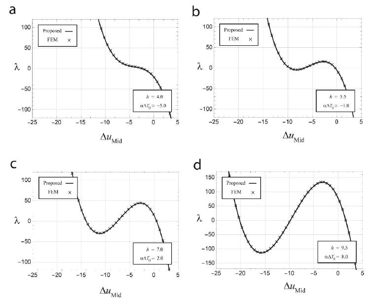
This equation is compatible with the results previously presented in the literature for a pin-ended shallow arch under a half-sine distributed loading (Plaut and Johnson, 1981). Eqs. (24) and (25) reveals the equilibrium path in the space $\text{(}\lambda \text{,}u\text{)}$ for the different values of $p$. For example, the displacement in the middle of the span ($\xi =\pi /2$) is equal to

$\Delta u_{Mid}=\Delta u(\pi /2)=\left(\frac{h-\lambda }{1+p}-h\right)$ (26)

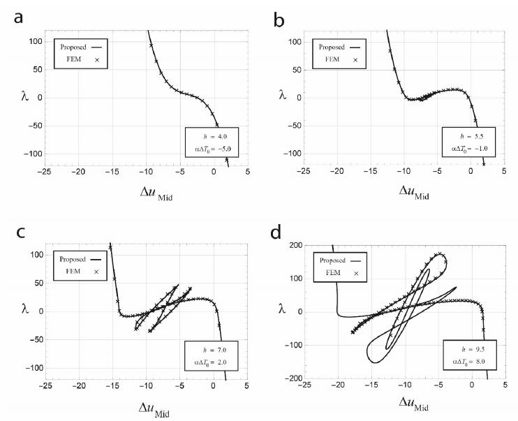
Figure 3 shows the equilibrium path for four different values of $h$ and$\alpha \Delta T_0$. In this diagram, the solid curves are the obtained initial equilibrium paths from Eqs. (24) and (26). In order to verify the suggested method, a non-linear FEM procedure is applied. In Figure 3, the signs $\times$ represent the structural responses obtained by FEM. Here, 60 Timoshenko beam elements with large displacements are used for modeling the shallow arch (Reddy, 2004). Each element includes six DoFs in the space of $\text{(}\xi \text{,}u\text{)}$. The equilibrium paths are traced by an incremental-iterative procedure (Crisfield, 1991; Crisfield, 1997). In this way, a modified cylindrical arc-length method is applied to find the next static state from the previous one (Moghaddasie and Stanciulescu, 2013a; Rezaiee-Pajand and Moghaddasie, 2014). The procedure of non-linear FEM begins from the initial unloaded state ($\lambda =0$) and traces the equilibrium path for both directions $\lambda >0$ and $\lambda <0$. All calculations were performed with the software Wolfram Mathematica 10.

Figure 3
Initial equilibrium paths for four different values of $h$ and $\alpha \Delta T_0$

The comparison between the formation of curves and the result of finite element method displays the performance of the proposed strategy. It is noteworthy that the non-linear FEM procedure obtains a number of discrete equilibrium points, while a continuous equilibrium curve is given by the suggested method.

As it is mentioned previously, there is a non-zero term in bifurcation paths (${\alpha }_j\ne 0$). From Eq. (13), the value $p$is obtained ($p=-j^2$), and by considering Eq. (12), the magnitude of ${\alpha }_j$is calculated:

${\alpha }_j=\pm \frac{2}{j}\sqrt{\alpha \Delta T_0+\frac{h^2}{4}-j^2-\frac{{(h-\lambda )}^2}{4{(1-j^2)}^2}},j=\mathrm{2,3,}\dots$ (27)

Similar to the initial equilibrium path, the displacement field relative to the $j$th bifurcation path is obtained by substituting the coefficients ${\alpha }_n$ into Eq. (8):

$\Delta u_j\left(\xi \right)=(\frac{h-\lambda }{1-j^2}-h)\sin \xi +{\alpha }_j\sin j\xi ,j=\mathrm{2,3,...}$ (28)

This equation shows a linear relationship between $\lambda$ and $\Delta \text{u}$. By considering $\xi =\pi /2$, the displacement of the midpoint in the $j$th bifurcation path is computed:

$\Delta u_{jMid}=(\frac{h-\lambda }{1-j^2}-h)+{\alpha }_{j}sin\frac{\pi j}{2},\begin{array}{cc}& \end{array}j=\mathrm{2,3,...}$ (29)

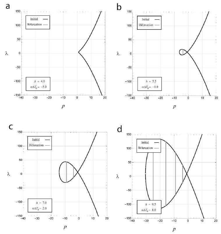
The gray curves in Figure 4 represent the calculated bifurcation paths given by Eq. (29).

Figure 4
Initial and bifurcation paths for different values of $h$ and $\alpha \Delta T_0$

As it can be seen, for greater values of $h$ and$\alpha \Delta T_0$, the number of bifurcation paths increases. This issue will be discussed later.

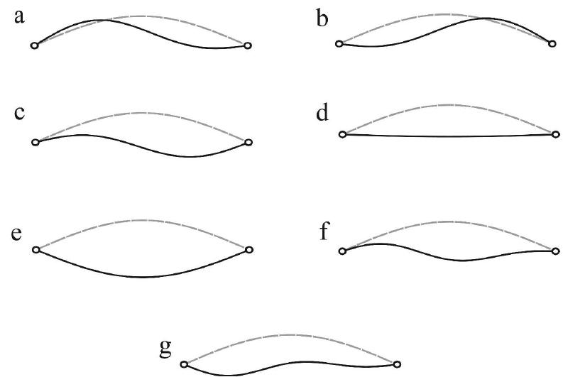
To investigate the structural behavior, a number of static states are displayed in Figure 5. These states are related to points a-g specified in Figure 4(b). In this Figure, the points a-c and d-g are, respectively, corresponding to the initial and bifurcation paths.

Figure 5
Equilibrium states corresponding to the points a-g shown in Figure 4(b)

A particular case which can be of interest is the relationship between the external load parameter and the axial force along the equilibrium path. Figure 6 draws this relationship by considering Eq. (23). In this figure, four cases corresponding to the values of $h$ and$\alpha \Delta T_0$ given in Figure 3(a)-(d) are shown.

Figure 6
Relationship between load parameter and axial force for four different values of $h$ and $\alpha \Delta T_0$

The solid black and gray curves are relative to the initial and bifurcated paths, respectively. Note that, negative values for the axial force $p$ represent that the shallow arch is in compression. As it is seen, the arch is always in tension for the case (a). By increasing the parameters $h$ and$\alpha \Delta T_0$, the magnitude of $p$ becomes negative in some parts of initial equilibrium paths. All bifurcation paths happen when the arch is in compression.

In order to obtain limit points, Eq. (19) can be rewritten in a simpler form:

$1+{\displaystyle \sum _{n=1}^{\infty }\begin{array}{c}\frac{{\alpha }_n^2}{{\beta }_{nn}}\end{array}}=0$ (30)

By substituting the obtained values ${\alpha }_n$ from Eq. (22) into Eq. (30), the critical load is calculated:

$1+\frac{{(h-{\lambda }_{cr})}^2}{2{(1+p)}^3}=0$ (31)

In this equation, ${\lambda }_{cr}$ represents the critical load. Eqs. (23) and (31) display the locus of limit points in the space $({\lambda }_{cr},\alpha \Delta T_0,h)$.

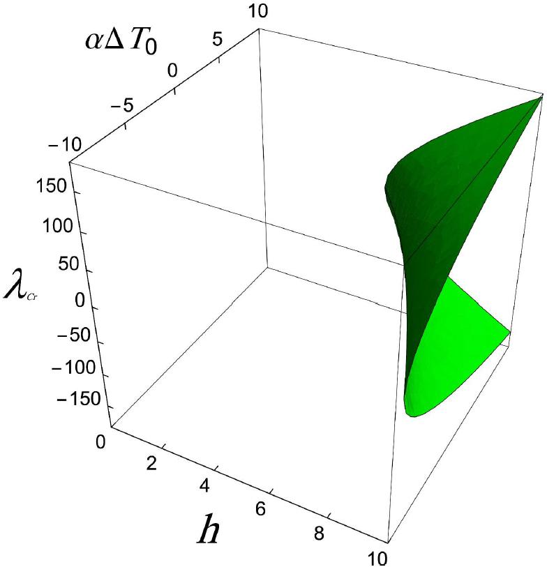
Figure 7 shows the relationship between the magnitude of critical load and the values of $h$ and$\alpha \Delta T_0$ for the interval $\{\left(h,\alpha \Delta T_0\right)\in {\text{R}}^2|0<h<\mathrm{10,}-10<\alpha \Delta T_0<10\}$. As it can be seen, depending on the values of $\alpha \Delta T_0$ and $h$, the equilibrium path can include zero or two points.

Figure 7
The locus of limit points in the space of $\left({\lambda }_{cr},\alpha \Delta T_0,h\right)$

The projection of the surfaces displayed in Figure 7 on the plane of $\left(h,\alpha \Delta T_0\right)$ draws a boundary which is identifying the number of limit points on the equilibrium path. Figure 8 illustrates the mentioned boundary and the locus of states (a)-(d) in Figure 3. As a result, the initial equilibrium paths corresponding to the upper side of the boundary (e.g. states (b)-(d)) include two limit points, while there is no limit point for the state (a). This issue would also be realized by the investigation of critical surfaces passing over the supposed $h$ and$\alpha \Delta T_0$ in Figure 7.

Figure 8
The boundary identifying the number of limit points in the space of $\left(h,\alpha \Delta T_0\right)$

It can be proven that the magnitude of the axial force on the boundary ($B_L$) is constant and equal to $-1$. By substituting the critical condition (31) into Eq. (23) and considering $p\to -1$, a relationship between the parameters $h$ and$\alpha \Delta T_0$ is obtained for the boundary $B_L$:

$B_L=\left\{\left(h,\alpha \Delta T_0\right)\in {\text{R}}^2|\alpha \Delta T_0=1-\frac{h^2}{4}\right\}$ (32)

As previously mentioned, the bifurcation points have the following characteristics:

$\{\begin{array}{c}{\alpha }_n=\mathrm{0,}n=\mathrm{2,3,...},n\ne j\\ p=-j^2,j=\mathrm{2,3,...}\end{array}$ (33)

Since bifurcation points are located on both initial and bifurcation paths, these points include all properties of both paths (especially, the condition ${\alpha }_j=0$). By considering Eq. (27), a relationship between $h$, $\alpha \Delta T_0$ and ${\lambda }_{cr}$ is obtained:

$c_j=\alpha \Delta T_0+\frac{h^2}{4}-j^2-\frac{{(h-{\lambda }_{cr})}^2}{4{\left(1-j^2\right)}^2}=\mathrm{0,}j=\mathrm{2,3,}\dots$ (34)

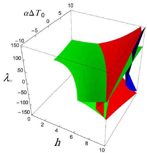
The equation $c_j=0$ provides surfaces in the space $({\lambda }_{cr},\alpha \Delta T_0,h)$. These surfaces describe the value of critical loads ${\lambda }_{cr}$corresponding to bifurcation points on the equilibrium path. According to the values of $h$ and $\alpha \Delta T_0$, the number of bifurcation points can be zero, two, four, six and eight. In Figure 9, the green, red, blue and yellow surfaces represent the magnitude of critical points corresponding to the first, second, third and fourth bifurcation paths, respectively.

Figure 9
The locus of bifurcation points in the space of $\left({\lambda }_{cr},\alpha \Delta T_0,h\right)$

In a similar way, the boundaries which are identifying the number of bifurcation points on the equilibrium path ($B_B$), can be derived by projecting the surfaces on the plane of $h$ and $\alpha \Delta T_0$. For this purpose, the constraint $\partial c_j/\partial {\lambda }_{cr}=0$ should be satisfied. This constraint concludes ${\lambda }_{cr}=h$. Consequently, the following formulation for the set of boundaries $B_B$ is obtained from (34):

$B_{Bj}=\left\{\left(h,\alpha \Delta T_0\right)\in {\text{R}}^2|\alpha \Delta T_0=j^2-\frac{h^2}{4}\right\},j=\mathrm{2,3,}\dots$ (35)

Figure 10 shows the boundaries $B_{Bj}$ for different values of $j$.

Figure 10
The boundaries identifying the number of bifurcation points in the space of $\left(h,\alpha \Delta T_0\right)$

It is noteworthy that, all initial equilibrium paths corresponding to the states between two specific curves include the same number of bifurcation points.

4.2 One-sine loading

Figure 1(c) shows the second loading type $Q_2=\lambda \sin 2\xi$. By substituting the value of $Q_2$ in Eq. (10), the magnitude of $q_n$ is obtained as follows:

$\{\begin{array}{c}{q}_1=-h\\ q_2=\lambda \\ q_n=0,n=\mathrm{3,4,....}\end{array}$ (36)

If the procedure, which is previously described in the Subsection 4.1, is applied, the values of ${\alpha }_n$ and $p$ will be calculated:

$\{\begin{array}{c}{\alpha }_1=\frac{h}{1+p}\\ {\alpha }_2=\frac{-\lambda }{16+4p}\\ \underset{}{\overset{}{{\alpha }_n}}=\mathrm{0,}n=\mathrm{3,4,...}\end{array}$ (37)

$p=-\alpha \Delta T_0-\frac{h^2}{4}+\frac{h^2}{4{\left(1+p\right)}^2}+\frac{{\lambda }^2}{{\left(16+4p\right)}^2}$ (38)

Additionally, the dimensionless displacement field for the initial equilibrium path is obtained from Eq. (8):

$\Delta u\left(\xi \right)=\left(-\frac{hp}{1+p}-\frac{2\lambda \cos \xi }{16+4p}\right)\sin \xi$ (39)

Consequently, the displacement of the midpoint is as follows:

$\Delta u_{Mid}=-\frac{hp}{1+p}$ (40)

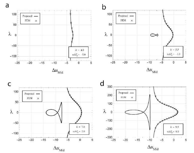
Figure 11 displays the equilibrium paths for four different values of $h$ and $\alpha \Delta T_0$. The comparison between the results given by the proposed method and the non-linear FEM shows the accuracy of the suggested technique. As it can be seen, for large values of $h$ and $\alpha \Delta T_0$, a secondary equilibrium path is appeared (Figure 11(b)-(d)). Since the procedure of FEM begins from the initial unloaded state (which is known a priori) and is capable to trace only the paths passing through this state, the secondary equilibrium paths cannot be achieved by FEM.

Figure 11
Initial and secondary equilibrium paths for four different values of $h$ and $\alpha \Delta T_0$

Similar to the Subsection 4.1., ${\alpha }_j$ can be obtained:

${\alpha }_j=\pm \frac{2}{j}\sqrt{\alpha \Delta T_0+\frac{h^2}{4}-j^2-\frac{h^2}{4{\left(1-j^2\right)}^2}-\frac{{\lambda }^2}{{\left(16-4j^2\right)}^2}},j=\mathrm{3,4,}\dots$ (41)

Eqs. (42) and (43), respectively, show the displacement field and displacement of the midpoint for the $j$th bifurcation state:

$\Delta u_j\left(\xi \right)=\left(\frac{h}{1-j^2}-\frac{2\lambda \cos \xi }{\left(16-4j^2\right)}-h\right)\sin \xi +{\alpha }_j\sin j\xi ,j=\mathrm{3,4,}\dots$ (42)

$\Delta u_{jMid}=\left(\frac{h{j}^2}{1-j^2}\right)+{\alpha }_j\sin \frac{\pi j}{2},j=\mathrm{3,4,}\dots$ (43)

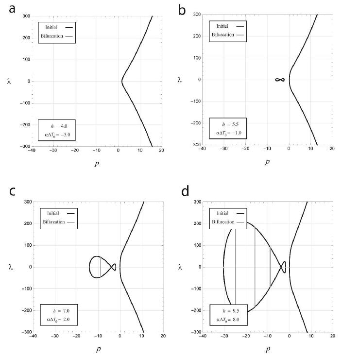
In Figure 12, bifurcation equilibrium paths are shown by gray curves. Although the initial equilibrium path does not include any critical point, the second path has limit and bifurcation points.

Figure 12
Initial, secondary and bifurcation paths for different values of $h$ and $\alpha \Delta T_0$

In addition, to have a better analogy, the relationship between the load parameter and the axial force is given in Figure 13.

Figure 13
Relationship between load parameter and axial force for four different values of $h$ and $\alpha \Delta T_0$

Figure 14 shows the equilibrium states relative to the points a-g in Figure 12(a).

Figure 14
Equilibrium states corresponding to the points a-g shown in Figure 12(a)

In order to obtain the locus of limit points, the values of ${\alpha }_n$ given by Eq. (37) are substituted into Eq. (30):

$1+\frac{h^2}{2{\left(1+p\right)}^3}+\frac{2{\lambda }_{cr}{}^2}{16{\left(4+p\right)}^3}=0$ (44)

Eqs. (38) and (44) reveal the location of limit points as a set of surfaces in the space of $({\lambda }_{cr},\alpha \Delta T_0,h)$. For the interval $\{\left(h,\alpha \Delta T_0\right)\in {\text{R}}^2|0<h<\mathrm{10,}-10<\alpha \Delta T_0<10\}$, the mentioned surfaces are shown in Figure 15. In this figure, each surface specifies a couple of critical points corresponding to the supposed $h$ and $\alpha \Delta T_0$.

Figure 15
The locus of limit points in the space of $\left({\lambda }_{cr},\alpha \Delta T_0,h\right)$

On the other hand, the equation (45) should be satisfied for the bifurcation points on the $j$th bifurcation path:

$\{\begin{array}{c}{\alpha }_n=\mathrm{0,}n=\mathrm{3,4,...},n\ne j\\ p=-j^2,j=\mathrm{3,4,...}\end{array}$ (45)

By considering $p=-j^2$ in Eq. (38), an explicit relationship between h, $\alpha \Delta T_0$ and ${\lambda }_{cr}$ is achieved:

$c_j=\alpha \Delta T_0+\frac{h^2}{4}-j^2-\frac{h^2}{4{\left(1-j^2\right)}^2}-\frac{{\lambda }_{cr}{}^2}{{\left(16-4j^2\right)}^2}=\mathrm{0,}j=\mathrm{3,4,}\dots$ (46)

Figure 16 shows surfaces $c_j=0$ for $\{\left(h,\alpha \Delta T_0\right)\in {\text{R}}^2|0<h<\mathrm{10,}-10<\alpha \Delta T_0<10\}$. The green, red and blue surfaces represent the magnitude of bifurcation points corresponding to the first, second and third bifurcated paths, respectively.

Figure 16
The locus of bifurcation points in the space of $\left({\lambda }_{cr},\alpha \Delta T_0,h\right)$

4.3 One and half-sine loading

If the loading pattern is assumed to be $Q_3=\lambda \sin 3\xi$ (Figure 1(d)), the values of $q_n$ and subsequently the magnitudes of ${\alpha }_n$ are obtained as follows:

$\{\begin{array}{c}{q}_1=-h\\ q_2=0\\ q_3=\lambda \\ q_n=\mathrm{0,}n=\mathrm{4,5,....}\end{array}$ (47)

$\{\begin{array}{c}{\alpha }_1=\frac{h}{1+p}\\ {\alpha }_2=0\\ {\alpha }_3=\frac{-\lambda }{9\left(9+p\right)}\\ {\alpha }_n=\mathrm{0,}n=\mathrm{4,5,...}\end{array}$ (48)

Furthermore, the calculated parameters $p$, $\Delta u$ and $\Delta u_{Mid}$ are respectively given by Eqs. (49)-(51):

$p=-\alpha \Delta T_0-\frac{h^2}{4}+\frac{h^2}{4{\left(1+p\right)}^2}+\frac{{\lambda }^2}{36{\left(9+p\right)}^2}$ (49)

$\Delta u\left(\xi \right)=-\frac{hp}{1+p}\sin \xi -\frac{\lambda }{9\left(9+p\right)}\sin 3\xi$ (50)

$\Delta u_{Mid}=-\frac{hp}{1+p}+\frac{\lambda }{9\left(9+p\right)}$ (51)

Figure 17 shows the equilibrium paths for four different values of $h$ and $\alpha \Delta T_0$. The solid curves and the signs $\times$, respectively, represent the obtained responses of the proposed technique and the finite element method.

Figure 17
Initial and secondary equilibrium paths for four different values of $h$ and $\alpha \Delta T_0$

In a similar way, the displacement field and displacement of midpoint for the $j$th bifurcation path can be calculated:

$\Delta u_j\left(\xi \right)=\frac{h{j}^2}{1-j^2}\sin \xi -\frac{\lambda }{9\left(9-j^2\right)}\sin 3\xi +{\alpha }_j\sin j\xi ,j=\mathrm{2,4,5,...}$ (52)

$\Delta u_{jMid}=\frac{h{j}^2}{1-j^2}+\frac{\lambda }{9\left(9-j^2\right)}+{\alpha }_j\sin \frac{\pi j}{2},j=\mathrm{2,4,5,...}$ (53)

By considering Eq. (12), ${\alpha }_j$is computed:

${\alpha }_j=\pm \frac{2}{j}\sqrt{\alpha \Delta T_0+\frac{h^2}{4}-j^2-\frac{h^2}{4{\left(1-j^2\right)}^2}-\frac{{\lambda }^2}{36{\left(9-j^2\right)}^2}},j=\mathrm{2,4,5,...}$ (54)

In Figure 18, the bifurcation paths are denoted by gray curves.

Figure 18
Initial, secondary and bifurcation paths for different values of $h$ and $\alpha \Delta T_0$

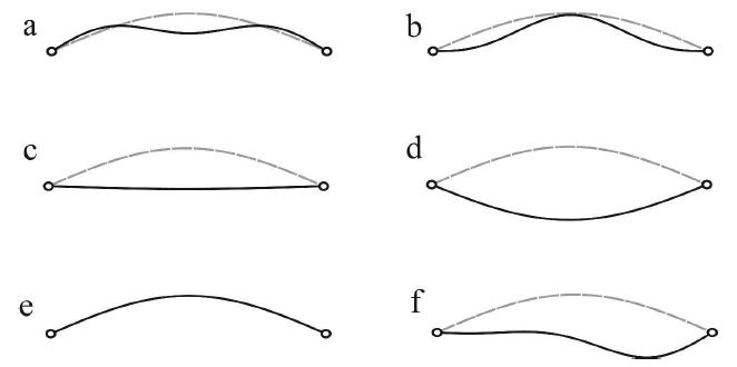
Figure 19 shows the structural states corresponding to the points a-f in Figure 18(b). Here, Figure 19(a)-(e) are relative to the initial and secondary equilibrium paths, while the last figure is related to the bifurcation path.

Figure 19
Equilibrium states corresponding to the points a-f shown in Figure 18(b)

Figure 18 shows that the initial equilibrium path does not include any critical point, and all critical points (limit and bifurcation) are located on the second equilibrium path. By substituting the values of ${\alpha }_n$ into Eq. (30), the critical load is calculated:

$1+\frac{h^2}{2{\left(1+p\right)}^3}+\frac{{\lambda }_{cr}{}^2}{18{\left(9+p\right)}^3}=0$ (55)

The locus of limit points in the interval $\{\left(h,\alpha \Delta T_0\right)\in {\text{R}}^2|0<h<\mathrm{10,}-10<\alpha \Delta T_0<10\}$ is presented in Figure 20:

Figure 20
The locus of limit points in the space of $\left({\lambda }_{cr},\alpha \Delta T_0,h\right)$

On the other hand, the bifurcation points should satisfy the following conditions:

$\{\begin{array}{c}{\alpha }_n=\mathrm{0,}n=\mathrm{2,4,5,...,}n\ne j\\ p=-j^2,j=\mathrm{2,4,5,...}\end{array}$ (56)

By substituting the value $p$ from Eq. (56) into Eq. (49), the location of bifurcation points in the space of $({\lambda }_{cr},\alpha \Delta T_0,h)$ is obtained:

$c_j=\alpha \Delta T_0+\frac{h^2}{4}-j^2-\frac{h^2}{4{\left(1-j^2\right)}^2}+\frac{{\lambda }_{cr}{}^2}{4\left(9-j^2\right)}=\mathrm{0,}j=\mathrm{2,4,5,...}$ (57)

The locus of bifurcation points for the interval $\{\left(h,\alpha \Delta T_0\right)\in {\text{R}}^2|0<h<\mathrm{10,}-10<\alpha \Delta T_0<10\}$ is shown in Figure 21. The green, red and blue surfaces represent the magnitude of bifurcation points corresponding to the first, second and third bifurcated paths, respectively.

Figure 21
The locus of bifurcation points in the space of $\left({\lambda }_{cr},\alpha \Delta T_0,h\right)$

4.4 k-sine loading

In this subsection, the effect of general sinusoidal loading pattern ($Q_k=\lambda \sin k\xi$) on the structural behavior of the shallow arch is investigated. The parameter $k$ describes the formation of the external loading. Based on this supposition, the magnitude of $q_n$ for $n=\mathrm{1,2,3,}\dots$ can be calculated for different values of $k$:

$k=1:\{\begin{array}{c}{q}_1=\lambda -h,n=1\\ q_n=\mathrm{0,}n=\mathrm{2,3,}\dots \end{array}$ (58)

$k=\mathrm{2,3,...}:\{\begin{array}{c}{q}_1=-h,n=1\\ q_n=\mathrm{0,}n=\mathrm{2,3,...},n\ne k\\ q_k=\lambda \end{array}$ (59)

By considering Eqs. (13), (58) and (59), the coefficients ${\alpha }_n$ are obtained in a generalized form:

$\text{(I):}\{\begin{array}{l}{\alpha }_1=\frac{h-\lambda }{1+P}\\ {\alpha }_n=0,n=\mathrm{2,3,}\dots \end{array}$ (60)

$\text{(II):}\{\begin{array}{l}{\alpha }_1=\frac{h-\lambda }{1+p}\\ {\alpha }_n=\mathrm{0,}n=\mathrm{2,3,...},n\ne j\\ {\alpha }_j\underset{}{\overset{}{from}}p=-j^2\end{array}$ (61)

$\text{(III):}\{\begin{array}{l}{\alpha }_1=\frac{h}{1+p}\\ {\alpha }_n=\mathrm{0,}n=\mathrm{2,3,...},n\ne k\\ {\alpha }_k=-\frac{\lambda }{k^2(k^2+p)}\end{array}$ (62)

$\text{(IV):}\{\begin{array}{l}{\alpha }_1=\frac{h}{1+p}\\ {\alpha }_n=\mathrm{0,}n=\mathrm{2,3,...},n\ne k,n\ne j\\ {\alpha }_k=-\frac{\lambda }{k^2(k^2+p)}\\ {\alpha }_{j}fromp=-j^2\end{array}$ (63)

The States I and II are corresponding to $k=1$, while the others are relative to the condition $k>1$. Additionally, the States I and III can describe the initial equilibrium path. For this purpose, the magnitude of axial force is calculated by substituting Eqs. (60) and (62) into (12):

$\text{(I):}p=-\alpha \Delta T_0-\frac{h^2}{4}+\frac{{\left(h-\lambda \right)}^2}{4{(1+p)}^2}$ (64)

$\text{(III):}p=-\alpha \Delta T_0-\frac{h^2}{4}+\frac{h^2}{4{(1+p)}^2}+\frac{{\lambda }^2}{4{\left(k^2\left(k^2+p\right)\right)}^2}$ (65)

Subsequently, the dimensionless displacement field for the initial equilibrium path is achieved by considering Eq.(8) for the States I and III:

$\text{(I):}\Delta u=\left(\frac{h-\lambda }{1+p}-h\right)\sin \xi$ (66)

$\text{(III):}\Delta u=\left(\frac{h}{1+p}-h\right)\sin \xi -\left(\frac{\lambda }{k^2{\left(k^2+p\right)}^2}\right)\sin k\xi$ (67)

On the other hand, the States II and IV, are corresponding to the bifurcation equilibrium path. Similarly, the displacement field for the $j$th bifurcation path can be derived:

$\text{(II):}\Delta u_j\left(\xi \right)=\left(\frac{h-\lambda }{1-j^2}-h\right)\sin \xi +{\alpha }_j\sin j\xi$ (68)

$\text{(IV):}\Delta u_j\left(\xi \right)=\left(\frac{h}{1-j^2}-h\right)\sin \xi -\left(\frac{\lambda }{k^2\left(k^2-j^2\right)}\right)\sin k\xi +{\alpha }_j\sin j\xi$ (69)

The displacement of the midpoint is obtained when $\xi =\pi /2$ for the four mentioned states. The parameter ${\alpha }_j$for the States II and IV are calculated by substituting Eqs. (61) and (63) into (12) and considering $p=-j^2$:

$\text{(II):}{\alpha }_j=\pm \frac{2}{j}\sqrt{\alpha \Delta T_0+\frac{h^2}{4}-j^2-\frac{{\left(h-\lambda \right)}^2}{4{\left(1-j^2\right)}^2}}$ (70)

$\text{(IV):}{\alpha }_j=\pm \frac{2}{j}\sqrt{\alpha \Delta T_0+\frac{h^2}{4}-j^2-\frac{h^2}{4{\left(1-j^2\right)}^2}-\frac{{\lambda }^2}{4k^2{\left(k^2-j^2\right)}^2}}$ (71)

In order to find limit points on the initial equilibrium path, Eq. (30) is applied:

$\text{(I):}1+\frac{{\left(h-{\lambda }_{cr}\right)}^2}{2{\left(1+p\right)}^3}=0$ (72)

$\text{(III):}1+\frac{h^2}{2{\left(1+p\right)}^3}+\frac{k^2{\lambda }_{cr}{}^2}{2\left(k^2+p\right){\left(k^2\left(k^2+p\right)\right)}^2}=0$ (73)

Furthermore, the condition (74) should be satisfied for the $j$th bifurcation point:

$\{\begin{array}{l}{\alpha }_n=\mathrm{0,}n=\mathrm{2,3,...,}n\ne k,n\ne j\\ p=-j^2,j=\mathrm{2,3,...,}j\ne k\end{array}$ (74)

By substituting Eq. (74) into Eqs. (64) and (65), the locus of bifurcation points is computed:

$\text{(I)}\text{,}\text{(II):}{c}_j=\alpha \Delta T_0+\frac{h^2}{4}-j^2-\frac{{\left(h-{\lambda }_{cr}\right)}^2}{4{\left(1-j^2\right)}^2}=0$ (75)

$\text{(III)}\text{,}\text{(IV):}{c}_j=\alpha \Delta T_0+\frac{h^2}{4}-j^2-\frac{h^2}{4{\left(1-j^2\right)}^2}-\frac{{\lambda }_{cr}{}^2}{4k^2{\left(k^2-j^2\right)}^2}=0$ (76)

It is noteworthy that bifurcation points are located on both initial and bifurcated paths.

4.5 Symmetric step loading

A type of symmetric step load is shown in Figure 1(e). This loading pattern can be defined in the following form:

$Q\left(\xi \right)=\{\begin{array}{l}00<\xi <0.25\pi \text{and}0.75\pi <\xi <\pi \\ \lambda 0.25\pi \le \xi \le 0.75\pi \end{array}$ (77)

By using the Fourier series, the values of $q_n$ for $n=\mathrm{1,2,...}$ are obtained:

$\{\begin{array}{c}{q}_1=\frac{2\sqrt{2}}{\pi }\lambda -h\begin{array}{cc}\begin{array}{ccc}& & \end{array}& \end{array}\begin{array}{cc}\begin{array}{ccc}& & \end{array}& \end{array}\\ q_n=\frac{4}{n\pi }\lambda \sin \frac{n\pi }{2}\sin \frac{n\pi }{4},\begin{array}{ccc}& & n=\mathrm{2,3,...}\end{array}\end{array}$ (78)

Note that for even values of $n$, the magnitude of $q_n$ is equal to zero. If the procedure, which is previously described, is applied, the values of ${\alpha }_n$ and $p$ will be calculated:

$\{\begin{array}{l}{\alpha }_1=-\frac{\frac{2\sqrt{2}}{\pi }\lambda -h}{1+p}\\ {\alpha }_n=-\frac{4\lambda \sin \frac{n\pi }{2}\sin \frac{n\pi }{4}}{\pi n^3\left(n^2+p\right)},\begin{array}{ccc}& & n=\mathrm{2,3,...}\end{array}\end{array}$ (79)

$p=-\alpha \Delta T_0-\frac{h^2}{4}+\frac{h^2}{4{\left(1+p\right)}^2}-\frac{\sqrt{2}h}{\pi {\left(1+p\right)}^2}\lambda +{\kappa }_{S,1}\left(p\right){\lambda }^2$ (80)

where, the function ${\kappa }_{S,i}\left(p\right)$ is defined in ^Appendix. The displacement field $\Delta u\left(\xi \right)$ and the displacement of the midpoint $\Delta u\left(\pi /2\right)$ for the initial equilibrium path are obtained from Eq. (8):

$\Delta u\left(\xi \right)=-\frac{hp}{1+p}\sin \xi +\lambda {\displaystyle \sum _{i=1}^{\infty }\left(\frac{-4\sin \frac{\left(2i-1\right)\pi }{2}\sin \frac{\left(2i-1\right)\pi }{4}}{\pi {\left(2i-1\right)}^3\left({\left(2i-1\right)}^2+p\right)}\right)\sin \left(2i-1\right)\xi }$ (81)

$\Delta u_{Mid}=-\frac{hp}{1+p}+{\kappa }_{S,2}\left(p\right)\lambda$ (82)

Figure 22 displays the equilibrium paths for four different values of $h$ and $\alpha \Delta T_0$. As it is seen, the procedure of FEM becomes divergent in the case of $h=9.5$ and $\alpha \Delta T_0=8.0$. This issue shows the efficiency of the proposed technique.

Figure 22
Initial equilibrium paths for four different values of $h$ and $\alpha \Delta T_0$

In the case of bifurcation path, there is a non-zero ${\alpha }_n$ for even values of $n$ (e.g., ${\alpha }_{2j}\ne 0$). Subsequently, the axial force is equal to $p=-4j^2$ based on Eq. (13). By considering Eq. (12), ${\alpha }_{2j}$ is achieved:

${\alpha }_{2j}=\pm \frac{1}{j}\sqrt{\alpha \Delta T_0+\frac{h^2}{4}-\frac{h^2}{4{\left(1-4j^2\right)}^2}+\frac{\sqrt{2}h}{\pi {\left(1-4j^2\right)}^2}\lambda -{\kappa }_{S,1}\left(-4j^2\right){\lambda }^2-4j^2},j=\mathrm{1,2,}\dots$ (83)

Eqs. (84) and (85), respectively, show the displacement field and displacement of the midpoint for the $j$th bifurcation state:

$\begin{array}{l}\Delta u_j\left(\xi \right)=\frac{4j^{2}h}{1-4j^2}\sin \xi +{\alpha }_{2j}\sin 2j\xi \\ +\lambda {\displaystyle \sum _{i=1}^{\infty }\left(\frac{-4\sin \frac{\left(2i-1\right)\pi }{2}\sin \frac{\left(2i-1\right)\pi }{4}}{\pi {\left(2i-1\right)}^3\left({\left(2i-1\right)}^2-4j^2\right)}\right)\sin \left(2i-1\right)\xi },j=\mathrm{1,2,}\dots \end{array}$ (84)

$\Delta u_{jMid}=\frac{4j^{2}h}{1-4j^2}+{\kappa }_{S,2}\left(-4j^2\right)\lambda ,j=\mathrm{1,2,}\dots$ (85)

In Figure 23, the bifurcation paths are given.

Figure 23
Initial and bifurcation paths for different values of $h$ and $\alpha \Delta T_0$

By substituting the values of ${\alpha }_n$ into Eq. (30), the critical load is calculated:

$1+\frac{h^2}{2{\left(1+p\right)}^3}-\frac{2\sqrt{2}h}{\pi {\left(1+p\right)}^3}{\lambda }_{cr}+{\kappa }_{S,3}\left(p\right){\lambda }_{cr}{}^2=0$ (86)

The locus of limit points in the interval $\{\left(h,\alpha \Delta T_0\right)\in {\text{R}}^2|0<h<\mathrm{10,}-10<\alpha \Delta T_0<10\}$ is presented in Figure 24. In this figure, each surface demonstrates a couple of limit points corresponding to the specific $h$ and $\alpha \Delta T_0$.

Figure 24
The locus of limit points in the space of $\left({\lambda }_{cr},\alpha \Delta T_0,h\right)$

On the other hand, by substituting the value $p=-4j^2$ into Eq. (80), the location of bifurcation points in the space of $({\lambda }_{cr},\alpha \Delta T_0,h)$ is obtained:

$c_j=\alpha \Delta T_0+\frac{h^2}{4}-\frac{h^2}{4{\left(1-4j^2\right)}^2}+\frac{\sqrt{2}h}{\pi {\left(1-4j^2\right)}^2}{\lambda }_{cr}-{\kappa }_{S,1}\left(-4j^2\right){\lambda }_{cr}{}^2-4j^2=\mathrm{0,}j=\mathrm{1,2,...}$ (87)

The locus of bifurcation points for the interval $\{\left(h,\alpha \Delta T_0\right)\in {\text{R}}^2|0<h<\mathrm{10,}-10<\alpha \Delta T_0<10\}$ is shown in Figure 25. The green and red surfaces represent the magnitude of bifurcation points corresponding to the first and second bifurcated paths, respectively.

Figure 25
The locus of bifurcation points in the space of $\left({\lambda }_{cr},\alpha \Delta T_0,h\right)$

4.6 Asymmetric step loading

An asymmetric step load is shown in Figure 1(f). This loading pattern is defined as

$Q\left(\xi \right)=\{\begin{array}{l}\lambda 0\le \xi \le 0.5\pi \\ 00.5\pi <\xi <\pi \end{array}$ (88)

The values of $q_n$ for $n=\mathrm{1,2,...}$ are achieved by using the Fourier series:

$\{\begin{array}{c}{q}_1=\frac{2}{\pi }\lambda -h\begin{array}{cc}\begin{array}{ccc}& & \end{array}& \end{array}\begin{array}{cc}\begin{array}{ccc}& & \end{array}& \end{array}\\ q_n=\frac{4}{n\pi }\lambda {\left(\sin \frac{n\pi }{4}\right)}^2,\begin{array}{ccc}& & n=\mathrm{2,3,...}\end{array}\end{array}$ (89)

It is noteworthy that the magnitude of $q_n$ is equal to zero when $n=4j$ (for $j=\mathrm{1,2,}\dots$). Similar to Subsection 4.5, the values of ${\alpha }_n$ and $p$ can be calculated:

$\{\begin{array}{l}{\alpha }_1=-\frac{\frac{2\text{}}{\pi }\lambda -h}{1+p}\\ {\alpha }_n=-\frac{4\lambda {\left(\sin \frac{n\pi }{4}\right)}^2}{\pi n^3\left(n^2+p\right)},\begin{array}{ccc}& & n=\mathrm{2,3,...}\end{array}\end{array}$ (90)

$p=-\alpha \Delta T_0-\frac{h^2}{4}+\frac{h^2}{4{\left(1+p\right)}^2}-\frac{h}{\pi {\left(1+p\right)}^2}\lambda +{\kappa }_{A,1}\left(p\right){\lambda }^2$ (91)

where, the function ${\kappa }_{A,i}\left(p\right)$ is defined in ^Appendix. Subsequently, the values of $\Delta u\left(\xi \right)$ and $\Delta u_{Mid}$ for the initial equilibrium path are

$\begin{array}{l}\Delta u\left(\xi \right)=-\frac{hp}{1+p}\sin \xi +\lambda {\displaystyle \sum _{i=1}^{\infty }\left(\frac{-2}{\pi {\left(2i-1\right)}^3\left({\left(2i-1\right)}^2+p\right)}\right)\sin \left(2i-1\right)\xi }\\ +\lambda {\displaystyle \sum _{i=1}^{\infty }\left(\frac{-4}{\pi {\left(4i-2\right)}^3\left({\left(4i-2\right)}^2+p\right)}\right)\sin \left(4i-2\right)\xi }\end{array}$ (92)

$\Delta u_{Mid}=-\frac{hp}{1+p}+{\kappa }_{A,2}\left(p\right)\lambda$ (93)

The initial equilibrium paths for different values of $h$ and $\alpha \Delta T_0$ are drawn in Figure 26.

Figure 26
Initial equilibrium paths for four different values of $h$ and $\alpha \Delta T_0$

As it is observed, the procedure of FEM becomes divergent in Figure 26(d).

In the case of asymmetric loading, there can be a non-zero ${\alpha }_{4j}$ for the $j$th bifurcation path. Consequently, the axial force $p$ equals $-16j^2$ according to Eq. (13). By considering Eq. (12), ${\alpha }_{4j}$ will be obtained:

$\begin{array}{l}{\alpha }_{4j}=\frac{1}{2j}(\alpha \Delta T_0+\frac{h^2}{4}-\frac{h^2}{4{\left(1-16j^2\right)}^2}\\ {+\frac{h}{\pi {\left(1-16j^2\right)}^2}\lambda -{\kappa }_{A,1}\left(-16j^2\right){\lambda }^2-16j^2)}^{1/2},j=\mathrm{1,2,}\dots \end{array}$ (94)

Accordingly, the displacement field and displacement of the midpoint for the $j$th bifurcation state are as follows:

$\begin{array}{l}\Delta u\left(\xi \right)=\frac{16j^{2}h}{1-16j^2}\sin \xi +\lambda {\displaystyle \sum _{i=1}^{\infty }\left(\frac{-2}{\pi {\left(2i-1\right)}^3\left({\left(2i-1\right)}^2-16j^2\right)}\right)\sin \left(2i-1\right)\xi }\\ +{\alpha }_{4j}\sin 4j\xi +\lambda {\displaystyle \sum _{i=1}^{\infty }\left(\frac{-4}{\pi {\left(4i-2\right)}^3\left({\left(4i-2\right)}^2-16j^2\right)}\right)\sin \left(4i-2\right)\xi },j=\mathrm{1,2,}\dots \end{array}$ (95)

$\Delta u_{Mid}=\frac{16j^{2}h}{1-16j^2}+{\kappa }_{A,2}\left(-16j^2\right)\lambda$ (96)

In the asymmetric step loading, there is only one bifurcation path which can be seen in the case of $h=9.5$ and $\alpha \Delta T_0=8.0$ (the gray solid curve in Figure 27).

Figure 27
Initial and bifurcation paths for $h=9.5$ and $\alpha \Delta T_0=8.0$

Similar to the previous subsection, the locus of limit points can be determined. In this way, the critical constraint (30) is rewritten in the following form by considering Eq. (90):

$1+\frac{h^2}{2{\left(1+p\right)}^3}-\frac{2h}{\pi {\left(1+p\right)}^3}{\lambda }_{cr}+{\kappa }_{A,3}\left(p\right){\lambda }_{cr}{}^2=0$ (97)

The locus of limit points in the interval $\{\left(h,\alpha \Delta T_0\right)\in {\text{R}}^2|0<h<\mathrm{10,}-10<\alpha \Delta T_0<10\}$ is shown in Figure 28. As it is observed, based on the magnitude of $h$ and $\alpha \Delta T_0$, the number of limit points could be zero, two, four, six or eight along the corresponding equilibrium path for this interval.

Figure 28
The locus of limit points in the space of $\left({\lambda }_{cr},\alpha \Delta T_0,h\right)$

In order to find the location of bifurcation points in the space of $({\lambda }_{cr},\alpha \Delta T_0,h)$, Eq. (91) with the constraint $p=-16j^2$ is applied:

$\begin{array}{l}{c}_j=\alpha \Delta T_0+\frac{h^2}{4}-\frac{h^2}{4{\left(1-16j^2\right)}^2}\\ +\frac{h}{\pi {\left(1-16j^2\right)}^2}{\lambda }_{cr}-{\kappa }_{A,1}\left(-16j^2\right){\lambda }_{cr}{}^2-16j^2=\mathrm{0,}j=\mathrm{1,2,...}\end{array}$ (98)

The locus of bifurcation points for the interval $\{\left(h,\alpha \Delta T_0\right)\in {\text{R}}^2|0<h<\mathrm{10,}-10<\alpha \Delta T_0<10\}$ is shown in Figure 29.

Figure 29
The locus of bifurcation points in the space of $\left({\lambda }_{cr},\alpha \Delta T_0,h\right)$

5 CONCLUSIONS

The stability behavior of shallow arches is always being of the researchers’ interest. In this paper, an analytical method to find the exact solution of a half-sinusoidal elastic shallow arch in the thermal environment under sinusoidal and step loads is proposed. For this purpose, the structural displacement is rewritten in a form of Fourier series, and subsequently, both initial and bifurcated equilibrium paths are obtained by substituting the transformed displacements into the governing equations of the arch. In addition, the critical points (such as limit and bifurcation points) are calculated by equating the determinant of stiffness matrix to zero. Furthermore, a new generalized formulation for various types of sinusoidal loadings is proposed.

In this research, the stability behavior of a half-sine shallow arch under three types of sinusoidal and two types of step function loads is separately investigated. Simultaneously, a non-linear finite element method is applied to show the accuracy and robustness of the suggested approach. In some cases, FEM becomes divergent during the path following procedure, while the proposed method is able to obtain the equilibrium path(s) comprehensively. Moreover, finding the critical points without tracing the equilibrium path is the superiority of the suggested technique.

Acknowledgements

The authors gratefully acknowledge the helpful suggestions received from the anonymous reviewers. The quality of this article has benefited substantially from their comments.

References

• Bateni, M. and Eslami, M.R. (2015). Non-linear in-plane stability analysis of FG circular shallow arches under uniform radial pressure, Thin-Walled Structures 94: 302-313.
• Bradford, M.A., Pi, Y.-L., Yang, G. and Fan, X.-C. (2015). Effects of approximations on non-linear in-plane elastic buckling and postbuckling analyses of shallow parabolic arches, Engineering Structures 101: 58-67.
• Cai, J., Xu, Y., Feng, J. and Zhang, J. (2012). In-plane elastic buckling of shallow parabolic arches under an external load and temperature changes, Journal of structural engineering 138(11): 1300-1309.
• Chandra, Y., Stanciulescu, I., Eason, T. and Spottswood, M. (2012). Numerical pathologies in snap-through simulations, Engineering Structures 34: 495-504.
• Chen, J.S. and Hung, S.Y. (2012). Exact snapping loads of a buckled beam under a midpoint force, Applied Mathematical Modelling 36: 1776-1782.
• Chen, J.S. and Li, Y.T. (2006). Effects of elastic foundation on the snap-through buckling of a shallow arch under a moving point load, International Journal of Solids and Structures 43(14): 4220-4237.
• Chen, J.S. and Liao, C.Y. (2005). Experiment and analysis on the free dynamics of a shallow arch after an impact load at the end, ASME Journal of Applied Mechanics 72(1): 54-61.
• Chen, J.S. and Lin, J.S. (2005). Exact critical loads for a pinned half-sine arch under end couples, ASME Journal of Applied Mechanics 72(1): 147-148.
• Chen, J.S. and Ro, W.C. (2009). Dynamic response of a shallow arch under end moments, Journal of Sound and Vibration 326(1): 321-331.
• Chen, J.S., Ro, W.C. and Lin, J.S. (2009). Exact static and dynamic critical loads of a sinusoidal arch under a point force at the midpoint, International Journal of Non-Linear Mechanics 44(1): 66-70.
• Chen, J.S. and Yang, C.H. (2007a). Experiment and theory on the nonlinear vibration of a shallow arch under harmonic excitation at the end, ASME Journal of Applied Mechanics 74(1): 1061-1070.
• Chen, J.S. and Yang, M.R. (2007b). Vibration and stability of a shallow arch under a moving mass-dashpot-spring system, ASME Journal of Vibration and Acoustics 129: 66-72.
• Crisfield, M.A. (1991). Non-linear Finite Element Analysis of Solids and Structures, Volume 1: Essentials, J. Wiley and Sons, Chichester.
• Crisfield, M.A. (1997). Non-linear Finite Element Analysis of Solids and Structures, Volume 2: Advanced Topics, J. Wiley and Sons, Chichester.
• Eriksson, A., Pacoste, C. and Zdunek, A. (1999). Numerical analysis of complex instability behaviour using incremental-iterative strategies, Computer methods in applied mechanics and engineering 179(3-4): 265-305.
• Han, Q., Cheng, Y., Lu, Y., Li, T. and Lu, P. (2016). Nonlinear buckling analysis of shallow arches with elastic horizontal supports, Thin-Walled Structures 109: 88-102.
• Hung, S.Y. and Chen, J.S. (2012). Snapping of a buckled beam on elastic foundation under a midpoint force, European Journal of Mechanics-A/Solids 31(1): 90-100.
• Khalil, H.K. (2002). Nonlinear Systems, Prentice Hall.
• Kiani, Y. and Eslami, M.R. (2013). Thermomechanical buckling of temperature-dependent FGM beams, Latin American Journal of Solids and Structures 10: 223-246.
• Matsunaga, H. (1996). In-plane vibration and stability of shallow circular arches subjected to axial forces, International Journal of Solids and Structures 33(4): 469-482.
• Moghaddasie, B. and Stanciulescu, I. (2013a). Direct calculation of critical points in parameter sensitive systems, Computers & Structures 117: 34-47.
• Moghaddasie, B. and Stanciulescu, I. (2013b). Equilibria and stability boundaries of shallow arches under static loading in a thermal environment, International Journal of Non-Linear Mechanics 51: 132-144.
• Moon, J., Yoon, K.Y., Lee, T.H. and Lee, H.E. (2007). In-plane elastic buckling of pin-ended shallow parabolic arches, Engineering Structures 29(10): 2611-2617.
• Pi, Y.-L. and Bradford, M.A. (2012). Non-linear buckling and postbuckling analysis of arches with unequal rotational end restraints under a central concentrated load, International Journal of Solids and Structures 49(26): 3762-3773.
• Pi, Y.-L. and Bradford, M.A. (2013). Nonlinear elastic analysis and buckling of pinned-fixed arches, International Journal of Mechanical Sciences 68: 212-223.
• Pi, Y.-L., Bradford, M.A. and Qu, W. (2010). Energy approach for dynamic buckling of shallow fixed arches under step loading with infinite duration, Structural Engineering and Mechanics 35(5): 555-570.
• Pi, Y.-L., Bradford, M.A. and Tin-Loi, F. (2007). Nonlinear analysis and buckling of elastically supported circular shallow arches, International Journal of Solids and Structures 44(7-8): 2401-2425.
• Pi, Y.-L., Bradford, M.A. and Tin-Loi, F. (2008). Non-linear in-plane buckling of rotationally restrained shallow arches under a central concentrated load, International Journal of Non-Linear Mechanics 43(1): 1-17.
• Pi, Y.-L., Bradford, M.A. and Uy, B. (2002). In-plane stability of arches, International Journal of Solids and Structures 39(1): 105-125.
• Pippard, A.B. (1990). The elastic arch and its modes of instability, European Journal of Physics 11: 359-365.
• Plaut, R.H. (2009). Snap-through of shallow elastic arches under end moments, ASME Journal of Applied Mechanics 76: 014504.
• Plaut, R.H. and Johnson, E.R. (1981). The effects of initial thrust and elastic foundation on the vibration frequencies of a shallow arch, Journal of Sound and Vibration 78(4): 565-571.
• Reddy, B.D. and Volpi, M.B. (1992). Mixed finite element methods for the circular arch problem, Computer methods in applied mechanics and engineering 97(1): 125-145.
• Reddy, J.N. (2004). An Introduction to Nonlinear Finite Element Analysis, Oxford University Press, USA.
• Rezaiee-Pajand, M. and Moghaddasie, B. (2014). Stability boundaries of two-parameter non-linear elastic structures, International Journal of Solids and Structures 51(5): 1089-1102.
• Rezaiee-Pajand, M. and Rajabzadeh-Safaei, N. (2016). An explicit stiffness matrix for parabolic beam element, Latin American Journal of Solids and Structures 13: 1782-1801.
• Saffari, H., Mirzai, N.M. and Mansouri, I. (2012). An accelerated incremental algorithm to trace the nonlinear equilibrium path of structures, Latin American Journal of Solids and Structures 9: 425-442.
• Stanciulescu, I., Mitchell, T., Chandra, Y., Eason, T. and Spottswood, M. (2012). A lower bound on snap-through instability of curved beams under thermomechanical loads, International Journal of Non-Linear Mechanics 47(5): 561-575.
• Thompson, J.M.T. and Hunt, G.W. (1973). A General Theory of Elastic Stability, J. Wiley.
• Tsiatas, G.C. and Babouskos, N.G. (2017). Linear and geometrically nonlinear analysis of non-uniform shallow arches under a central concentrated force, International Journal of Non-Linear Mechanics 92: 92-101.
• Virgin, L.N., Wiebe, R., Spottswood, S.M. and Eason, T.G. (2014). Sensitivity in the structural behavior of shallow arches, International Journal of Non-Linear Mechanics 58: 212-221.
• Xenidis, H., Morfidis, K. and Papadopoulos, P.G. (2013). Nonlinear analysis of thin shallow arches subject to snap-through using truss models, Structural Engineering and Mechanics 45(4): 521-542.
• Xu, J.X., Huang, H., Zhang, P.Z. and Zhou, J.Q. (2002). Dynamic stability of shallow arch with elastic supports-application in the dynamic stability analysis of inner winding of transformer during short circuit, International Journal of Non-Linear Mechanics 37(4): 909-920.
• Zhou, Y., Chang, W. and Stanciulescu, I. (2015a). Non-linear stability and remote unconnected equilibria of shallow arches with asymmetric geometric imperfections, International Journal of Non-Linear Mechanics 77: 1-11.
• Zhou, Y., Stanciulescu, I., Eason, T. and Spottswood, M. (2015b). Nonlinear elastic buckling and postbuckling analysis of cylindrical panels, Finite Elements in Analysis and Design 96: 41-50.

• Available online: June 06, 2018

APPENDIX

Here, the functions ${\kappa }_{S,i}\left(p\right)$ and ${\kappa }_{A,i}\left(p\right)$ are defined and their magnitudes are given for some values of $i$:

$\begin{array}{l}{\kappa }_{S,1}\left(p\right)={\displaystyle \sum _{i=1}^{\infty }\frac{2}{{\pi }^2{\left(2i-1\right)}^4{\left({\left(2i-1\right)}^2+p\right)}^2}}\\ =-\frac{1}{2p^3}+\frac{{\pi }^2}{48p^2}-\frac{{\left(\text{sech}\frac{\sqrt{p}\pi }{2}\right)}^2}{8p^3}+\frac{5\tanh \frac{\sqrt{p}\pi }{2}}{4p^{7/2}\pi }\end{array}$ (A.1)

$\begin{array}{l}{\kappa }_{S,2}\left(p\right)={\displaystyle \sum _{i=1}^{\infty }\frac{-4\sin \frac{\left(2i-1\right)\pi }{4}}{\pi {\left(2i-1\right)}^3\left({\left(2i-1\right)}^2+p\right)}}\\ =\frac{1}{p^2}-\frac{3{\pi }^2}{32p}-\frac{\cot \left(\frac{1}{8}\left(3+\sqrt{-p}\right)\pi \right)}{4\sqrt{2}{p}^2}-\frac{\csc \left(\frac{1}{4}\left(1+\sqrt{-p}\right)\pi \right)}{2\sqrt{2}{p}^2}-\frac{\tan \left(\frac{1}{8}\left(3+\sqrt{-p}\right)\pi \right)}{4\sqrt{2}{p}^2}\end{array}$ (A.2)

$\begin{array}{l}{\kappa }_{S,3}\left(p\right)={\displaystyle \sum _{i=1}^{\infty }\frac{4}{{\pi }^2{\left(2i-1\right)}^4{\left({\left(2i-1\right)}^2+p\right)}^3}}\\ =-\frac{3}{2p^4}+\frac{{\pi }^2}{24p^3}-\frac{11{\left(\text{sech}\frac{\sqrt{p}\pi }{2}\right)}^2}{16p^4}+\frac{35\tanh \frac{\sqrt{p}\pi }{2}}{8p^{9/2}\pi }-\frac{\pi {\left(\text{sech}\frac{\sqrt{p}\pi }{2}\right)}^2\tanh \frac{\sqrt{p}\pi }{2}}{16p^{7/2}}\end{array}$ (A.3)

$\begin{array}{l}{\kappa }_{A,1}\left(p\right)={\displaystyle \sum _{i=1}^{\infty }\frac{1}{{\pi }^2{\left(2i-1\right)}^4{\left({\left(2i-1\right)}^2+p\right)}^2}}+{\displaystyle \sum _{i=1}^{\infty }\frac{4}{{\pi }^2{\left(4i-2\right)}^4{\left({\left(4i-2\right)}^2+p\right)}^2}}\\ =-\frac{1}{2p^3}+\frac{5{\pi }^2}{384p^2}-\frac{{\left(\text{sech}\frac{\sqrt{p}\pi }{4}\right)}^2}{16p^3}-\frac{{\left(\text{sech}\frac{\sqrt{p}\pi }{2}\right)}^2}{16p^3}+\frac{5\tanh \frac{\sqrt{p}\pi }{4}}{4p^{7/2}\pi }+\frac{5\tanh \frac{\sqrt{p}\pi }{2}}{8p^{7/2}\pi }\end{array}$ (A.4)

$\begin{array}{l}{\kappa }_{A,2}\left(p\right)={\displaystyle \sum _{i=1}^{\infty }\frac{2{\left(-1\right)}^i}{\pi {\left(2i-1\right)}^3\left({\left(2i-1\right)}^2+p\right)}}\\ =-\frac{1}{2p^2}+\frac{{\pi }^2}{16p}+\frac{\text{sech}\frac{\sqrt{p}\pi }{2}}{2p^2}\end{array}$ (A.5)

$\begin{array}{l}{\kappa }_{A,3}\left(p\right)={\displaystyle \sum _{i=1}^{\infty }\frac{2}{{\pi }^2{\left(2i-1\right)}^4{\left({\left(2i-1\right)}^2+p\right)}^3}}+{\displaystyle \sum _{i=1}^{\infty }\frac{8}{{\pi }^2{\left(4i-2\right)}^4{\left({\left(4i-2\right)}^2+p\right)}^3}}\\ =-\frac{3}{2p^4}+\frac{5{\pi }^2}{192p^3}-\frac{11{\left(\text{sech}\frac{\sqrt{p}\pi }{4}\right)}^2}{32p^4}-\frac{11{\left(\text{sech}\frac{\sqrt{p}\pi }{2}\right)}^2}{32p^4}+\frac{35\tanh \frac{\sqrt{p}\pi }{4}}{8p^{9/2}\pi }\\ -\frac{\pi {\left(\text{sech}\frac{\sqrt{p}\pi }{4}\right)}^2\tanh \frac{\sqrt{p}\pi }{4}}{64p^{7/2}}+\frac{35\tanh \frac{\sqrt{p}\pi }{2}}{16p^{9/2}\pi }-\frac{\pi {\left(\text{sech}\frac{\sqrt{p}\pi }{2}\right)}^2\tanh \frac{\sqrt{p}\pi }{2}}{32p^{7/2}}\end{array}$ (A.6)

Publication Dates

• Publication in this collection
  2018

History

• Received
  22 Oct 2017
• Reviewed
  21 Jan 2018
• Accepted
  28 Feb 2018