MULTI-AGENT BASED MODELING APPLIED TO PORTFOLIO SELECTION IN THE DOOM-LOOP OF SOVEREIGN DEBT CONTEXT^**

ABSTRACT

This study explores the self-fulfilling dynamic between sovereign debt risk and rational choices of neutral, risk-seeking and risk-averse investors, with implications to the systemic risk emergence. The agent-based model parameterization includes investment strategy (randomly selected assets, stock exchange participation, economic segment, and technical analysis), portfolio rebalance period, and stop gain/loss option. We use Brazilian markets data from 2006 to 2017 to simulate stochastic distributions of investments by a set of 3,000 agents in both stages of model verification and validation (robustness check). Using the Capital Asset Pricing Model, we confirmed our proposition that the optimal rational risk attitude (less risk appetite) constitutes a trigger for the self-fulfilling dynamic, having its foundation on government securities yield and in the debt dynamics. This finding is contrary to the equity premium puzzle in the Brazilian case. The findings have implications to policymakers regarding systemic risk issues, among other public policies.

Keywords:
portfolio selection; agent-based model; sovereign debt; doom-loop; systemic risk

1 INTRODUCTION

Modern financial systems feature three noteworthy issues considered in this article: the increasing scarcity of deemed risk-free assets, which serve as reference points in economic and finance models, the financial instability generated by a self-fulfilling process of sovereign debts, sovereign spreads and bank ratings, and the systemic risk emergence process.

From the late 1990s to 2008, government bonds issued by European states showed all the characteristics of a risk-free asset. According to ^{Bowdler and Esteves (2013}), the ratio of sovereign debt to GDP for advanced economies has risen from about 50% in 2007 to 80% in 2012. In 2011, one of the major concerns was the systemic risk of the European banking system, where contagion fears spread among euro area investors, resulting in financial instability (^{Black, Correa,Huang & Zhou, 2016}). The euro-area sovereign debt crisis highlighted the nexus between government and banks and its powerful effects on lending and economic activity (^{Altavilla,Pagano & Simonelli, 2016}).

^{Gibson, Hall, and Tavlas (2017}) confirmed the interactions among sovereign spreads, sovereign credit ratings, and bank ratings: sovereign downgrades and rises in sovereign spreads led to downgrades of banks within the sovereign’s jurisdiction, and the bank downgrades contributed to both further sovereign downgrades and increases in spreads. The existence of negative feedback loops challenges the explanation of the movements in spreads based on fundamentals variables.

^{Brunnermeier, Langfield, Pagano, Reis, Van Nieuwerburgh, and Vayanos (2016}) describe the doom-loop between sovereign risk and bank risk as an initial economic shock generating loss in sovereign bonds in the asset side of bank’s balance sheet, feeding the cycle with negative outlook for the securities, affecting back the sovereign rating. Among the types of systemic risk, ^{Allen and Carletti (2013}) include sovereign defaults. In this research, we focus on the following question: could rational investment behavior lead to systemic risk?

A survey on systemic risk literature (^{Silva, Kimura & Sobreiro, 2017}) shows an intensification of articles focusing on systemic risk since the US mortgage crisis of 2007/8. Most research uses quantitative investigation methods, whereas computational simulation and agent-based models are useful approaches for the micro-macro interconnection analysis, and can be allied with quantitative methods. As pointed by the survey, only two out of the 266 articles used agent-based models. The ‘credit/counterparty/sovereign risks’ object of study accounts for 17% of the survey sample. Further, ^{Ashraf (2017}) argue that the last global financial crisis has urged to new research on bank risk-taking behavior, with the expansion of the literature examining country-level factors, such as political institutions.

The goal of this research is to explore the emergence of systemic risk as consequence of the mentioned doom-loop of the sovereign debt, using an agent-based model with three agent types: neutral, risk-seeking and risk-averse investors. Those investors choose portfolios of assets on a monthly basis, following rational options. Our proposition is that the optimal risk attitude constitutes a trigger for the feedback loop. To deal with this conjecture, we outline the following hypothesis:

• H1₀: Risk-seeking investors, who select higher associated risk and expected return portfolios compared to risk-averse investors, have better comparative performance, using a common market portfolio.

• H1_a: Risk-averse investors, who select lower associated risk and expected return portfolios compared to risk-seeking investors, have better comparative performance, using a common market portfolio.

The null hypothesis is based on the equity premium puzzle. ^{Mehra and Prescott (1985}) showed that, historically, the average return on equity has far exceeded the average return on short-term virtually default-free debt. From 1889 to 1978, the average real annual yield on the Standard and Poor 500 Index was seven percent, while the average yield on short-term debt was less than one percent, challenging general equilibrium models of asset pricing. In addition, in emerging markets the average equity premium is significantly higher than in developed markets, with some industries performing consistently better than others (^{Donadeli & Persha, 2014}).

Therefore, even though during crises time we can expect the investor’s attitude toward capital protection, we outline the alternative hypothesis to investigate a broad period that includes the last financial crisis. Using Brazilian market data from 2006 to 2017 and a set of 3,000 agents to generate stochastic distributions of portfolio realizations, we analyzed rational choices of investors with different risk appetite, based on portfolio selection theory (^{Markowitz, 1952}; ^{Sharpe, 1964}; ^{Lintner, 1965}). The results show that risk-averse investors had better performance than neutral and risk-seeking investors, mainly at times of political and economic uncertainties. This rationality can be seen as a potential initial shock in the doom-loop that connects sovereign and bank risks, which turns to a trigger to systemic risk.

Following this introduction, we present in section 2 a review of the related work. The section 3 explains the methodology of the study, with the high-level research model and the mainalgorithms. In the section 4, we discuss the results, and in the section 5, we conclude.

2 THEORETICAL BACKGROUND

In this section, we review the literature related to the research design, to the sovereign debt and systemic risk, and the problem of portfolio selection.

2.1 Research design

With different purpose, our research design is similar to ^{Feldman (2010}), ^{Cui, Wang, Ye & Yan (2012}); and ^{Rekik, Hachicha & Boujelbene (2014}) in some aspects. ^{Feldman (2010)} develop a two market agent-based model to study how global portfolio managers affect global financial crises and stability. The author describes the agent-based model approach as a way to capture complex behavior and dynamics in financial markets, which are modeled as interacting groups of learning and rational bounded agents whose behavior is captured mainly by running computer simulations. The base model in ^{Feldman (2010)} uses the Markowitz’s modern portfolio theory to simulate investment decisions. ^{Kolm, Tutuncu & Fabozzi (2014}) highlight that the Markowitz’s work has influence in researches and in the financial industry. Besides the so-called mean-variance optimization, our approach also uses the Capital Asset Pricing Model.

Different approaches to portfolio selection were implemented in some researches, as the use of itemsets (^{Baralis, Cagliero & Garza, 2017}), evolutionary algorithms (^{Macedo, Godinho & Alves, 2017}), genetic programming (^{Berutich, López, Luna & Quintana, 2016}), fuzzy modeling (^{Liu, 2011}), entropy-driven approach (^{Rodder, Gartner & Rudolph, 2010}; ^{Gartner, 2012}), neural networks (^{Ko & Lin, 2008}) and Bayesian analysis (^{Ferreira, Almeida Filho & Souza, 2009}).

The architecture in ^{Cui et al. (2012}) models three types of agents acting in an artificial stock market: stock agent, finance agent and investor agent, which can have rational or irrational behavior. The finance agent produces signals to the investor agents, who uses this information for fundamental analysis, and the rational agent can also use technical analysis to invest. In our model, the differences among the agents reflect their attitude towards risk: neutral, averse, and risk-seeking investors. To cope with the absence of information for fundamental analysis, we use stochastic simulation to achieve the investors’ probability density functions.

^{Rekik et al. (2014}) explore the market dynamics from a behavioral perspective, using the investors’ irrationality to explain financial anomalies in asset pricing models, with three types of investors in the agent-based model: fundamentalist, non-fundamentalist and loss adverse. Our intention is to analyze the rational behavior of the investor, having the trade-off between risk and return as a driving behavior.

2.2 Sovereign debt and systemic risk

One of the greatest challenges for the European Union is the scarcity of safe assets in the euro-area (^{Brunnermeier et al., 2016}) because of the growth rate in the Eurozone developing countries during the last two decades that has increased the demand for safe assets. The financial crisis of 2007/8 showed a movement toward assets deemed virtually risk-free, as a process of flight to quality for capital reallocation.

It is also important to note the bank regulatory framework regarding bonds of sovereign debt. Following Basel prudential criteria, bank regulators require banks to manage their assets risk in proportion to their own capital. Therefore, banks tend to hold a substantial part of government securities in their balance sheets, having a zero risk-weight for this asset class to compute capital requirements. To save capital, particularly during crises when capital is scarce and sovereign risk are elevated, banks are incentivized to hold government debt securities (^{ESRB, 2015}).

Euro area banks hold € 1.9 trillion of euro sovereign bonds. From those, just three members are maximum quality rated (triple-A): Germany, the Netherlands and Luxembourg. The face value of the EU governments bonds stood at € 2.6 trillion in 2015 (25% of euro area GDP), meanwhile the sovereign debt of the US stood at USD 19 trillion (105% of US GDP).

The Brazilian outstanding bonds was USD 937 billion in September 2016 (corresponding to 49% of the Brazilian GDP), with 95% of the total bonds stock issued in its own currency (Brazilian Real), yielding a mean real return of 5.95% per year to the investors. Financial institutions, pension funds and mutual investment funds hold each one around a quarter of the government securities. The mean value of the secondary market stood at USD 10 billion on a daily basis. Roughly, the bond stock is divided in 1/3 of each type: index-linked (consumer price), fixed rate, and floating rate (^{STN, 2016}).

2.2.1 The doom-loop of sovereign debt

A design of a new financial architecture is proposed by ^{Brunnermeier et al. (2016}), considering the securitization of sovereign bonds of euro area nation-states as a diversified portfolio. The proposal is a response to the open issue stated by the authors as the “diabolic loop” (Fig. 1). ^{Brunnermeier et al. (2016)} show this problematic cycle from a bank’s point of view, showing a typical balance sheet with loans and deposits and their impact in the propagation channels. We have introduced a general investor (which includes bank) that, before the doom-loop initiation, can accumulate sovereign bonds and other investments in the capital market.

Figure 1:
The sovereign-bank doom loop. Figure adapted (insertions are in italic) from ^{Brunnermeier et al. (2016}). Our research conjecture is that the increase in the sovereign debt risk that may affect negatively the banks’ balance sheets in the doom-loop can be related to the public debt dynamics. It is important to note that public debt dynamics accounts, basically, for the current stock of debt, economic growth and interest level variables.

^{Brunnermeier et al. (2016}) observe that the threat is due to empirical observations of banks preferences to hold claims on their own sovereign, particularly during crises. According to ^{Acharya and Rajan (2013}), in the stress-test data released by European regulators in 2010, banks of Greece, Ireland, Portugal, Spain and Italy held on average more than 60% of their government bonds in their own government bonds. Furthermore, ^{IMF (2017)} also shows the importance of the sovereign-bank interdependence.

This home bias creates a potent doom-loop between sovereign risk and bank risk (^{Brunnermeier et al., 2016}). Considering an initial economic shock, it would affect the sovereign risk that could reduce the market value of the bonds and cause, consequently, a loss in the bank book and market equity value. After that, two propagations channels would follow. The first loop operates via a bailout channel: the reduction in the solvency of banks raises the probability of a bailout, leading to an increasing sovereign risk and lowering bond prices. The second loopappears in the real economy: the reduction in the solvency of banks owing to the fall in sovereign bond prices prompts them to cut lending, reducing real activity, lowering tax revenues, and increasing sovereign risk further. This cyclical effect amplified the euro area sovereign debt crisis after 2009 (^{Brunnermeier et al., 2016}). In Ireland, Spain, Greece, Italy, Portugal and Belgium the debt dynamics threatened banks solvency and the domestic government guarantees becameless credible.

Regarding the public debt dynamics (^{IMF, 2017}), in a closed economy where sovereign debt is expressed in local currency, in a general case the current stock of debt would depend on the previous stock of debt, the nominal interest rate and the primary balance surplus (or deficit). The intertemporal solvency condition prevents a Ponzi scheme (infinite debt rolled over new debt) with the condition that the outstanding debt should be covered by the present value of future primary surpluses. Therefore, in the long run, the projections of the debt-to-GDP ratio rely on the real interest rate (r), the economic growth rate (g) and the primary balance. The variables r and g compound the automatic debt dynamics, and a sustainable path would occur when g>r.

2.2.2 Systemic risk

Systemic risk refers to the potential bankruptcy events of multiple banks, in a domino effect, that can cause huge losses to investors, governments and to the whole economy. There are four types of systemic risk (^{Allen & Carletti, 2013}): panics, banking crises due to asset price falls, contagion and foreign exchange mismatches in the banking system. The sovereign defaults are classified in the second type, as a part of the doom loop. The sovereign debt crises tend to be more costly than banking crises, which in turn tend to be more costly than currency crises (^{Laeven & Valencia, 2013}). Banking crises often precede or accompany sovereign debt crises (^{Reinhart & Rogoff, 2011}).

In 2011, one of the greatest concerns was the systemic risk of the European banking system (^{Black et al., 2016}), where the contagion fears spread among the euro area investors resulting in financial instability. To measure the systemic risk of European banks, ^{Black et al. (2016)} calculate a total distress insurance premium around € 500 billion, largely due to sovereign default risk. Beyond their utility as liquid assets in the economy, risk-free assets serve as an important part of daily operations in the financial markets, as in the Repo Market, where they are used by central clearing counterparties (CCP) in collateralized operations.

In 2009, the ECB hosted a workshop gathering together experts from central banks and international organizations in the fields of financial stability and payment system to focus on the financial sector as a network of financial agents (^{ECB, 2010}). The report states that policy makers were looking for new analytical tools that help to better identify, monitor and address sources of systemic risk. To tackle this shortcoming, agent-based modeling was considered a recent alternative approach, relying on algorithms and simulations, where simple decision-make rules can generate complex behavior at the system level. Some research using agent-based model have been applied to investigate the dynamic of financial markets (^{Ashraf, Gershman & Howitt, 2017}; ^{Ge, 2017}) and public policies to deal with banking crises and recessions (^{Dosi, Fagiolo, Napoletano, Roventini & Treibich, 2015}).

Our research aims to investigate the emergence of systemic risk regarding the doom-loop described by ^{Brunnermeier et al. (2016}) and ^{Gibson et al. (2017}), using an agent-based approach to model three types of agents: neutral, risk-seeking and risk-averse investors.

2.3 Portfolio selection

The quantification of the trade-off between risk and expected return is one of the most important issues of modern financial economics (^{Campbell, Lo & Mackinlay, 1997}). In spite of the common sense that suggest that risky investments such as stock market will generally yield higher returns than investments free of risk, it was only during the decade of 1960 that academic researchers developed seminal works comprising portfolio theory (^{Markowitz, 1952}; ^{Sharpe, 1964}; ^{Lintner, 1965}). The main concern was economic agents who act under uncertainty and could make use of sufficient computer and database resources in order to obtain diversification of investments to reduce uncertainty and maximize their expected utility function. The existence of uncertainty is essential to the analysis of rational investment behavior (^{Markowitz, 1952}).

Investors would optimally hold a mean-variance efficient portfolio: a mix of assets with the highest expected return for a certain level of variance. Given a vector ω of weights or investments proportions of each of the n assets to compound the portfolio, the expected return and the risk of this portfolio are respectively:

$E\left(R\right)={\displaystyle \sum _{i=1}^n{R}_i{\omega }_i}$ (1)

$V\left(R\right)={\displaystyle \sum _{i=1}^n{\displaystyle \sum _{j=1}^n{\omega }_i{\omega }_j{\sigma }_{ij}}}$ (2)

where R _i is the return of asset i and σ_ij is the covariance between the returns of assets i and j.

A portfolio p is the minimum-variance portfolio of all portfolios with mean return μ_p if its portfolio weight vector is the solution to this optimization:

$\begin{array}{l}\min {\omega }^{\text{'}}\Omega \omega \\ \text{s}\text{.t}\text{.}\begin{array}{c}\end{array}{\omega }^{\text{'}}\mu ={\mu }_p\text{and}{\omega }^{\text{'}}\iota \text{=1}\end{array}$ (3)

where ι is a vector of ones, μ is the vector of expected returns, and Ω is the variance-covariance matrix of returns.

Solving the equation (3) gives ω _p (^{Campbell et al., 1997}):

${\omega }_p=g+h{\mu }_p$ (4)

$g=\frac{1}{D}\left[B\left({\Omega }^{-1}\iota \right)-A\left({\Omega }^{-1}\mu \right)\right]$ (5)

$h=\frac{1}{D}\left[C\left({\Omega }^{-1}\mu \right)-A\left({\Omega }^{-1}\iota \right)\right]$ (6)

$A=\iota \text{'}{\Omega }^{-1}\mu ,\begin{array}{c}\end{array}B=\mu \text{'}{\Omega }^{-1}\mu ,\begin{array}{c}\end{array}C=\iota \text{'}{\Omega }^{-1}\iota ,\begin{array}{c}\end{array}D=BC-A^2$ (7)

The efficient frontier of portfolios suggested by Markowitz was improved with the introduction of a risk-free asset in the model known as Capital Asset Pricing Model (CAPM), given an opportunity to invest a proportion α of the resources in the risky assets and the proportion (1-α) in the risk-free asset (^{Sharpe, 1964}; ^{Lintner, 1965}).

The factors β measure the sensibility of return of each asset in relation to the return of a market portfolio, which is an ideal portfolio of all invested wealth,

${\beta }_i=\frac{{\sigma }_{im}}{{\sigma }_m^2}$ (8)

where m refers to the market portfolio.

Therefore, the expected return of any asset would be calculated as a function of its sensibility coefficient (β_i), of the risk-free asset return (R _f ) and of the expected return of the market portfolio (R _m ):

$E\left(R_i\right)=R_f+{\beta }_i\left[E\left(R_m\right)-R_f\right]$ (9)

The Figure 2 shows that with a risk-free asset, all efficient portfolios lie along the “security market line” from the risk-free asset through the portfolio q that is the tangency or market portfolio. From the point R _f to q there is a continuum of choices to the vector ω, with $0\le \alpha \le 1$. Specifically for the tangency portfolio, the proportion α is equal to one, and beyond this point, the investor would be willing to borrow at a risk-free rate of interest and reinvest this amount in risky assets.

The tangency portfolio weights ω _q can be obtained as follows:

${\omega }_q=\frac{1}{\iota \text{'}{\Omega }^{-1}\left(\mu -R_f\iota \right)}\cdot {\Omega }^{-1}\left(\mu -R_f\iota \right)$ (10)

Figure 2:
Efficient frontier with a risk-free asset. Figure adapted from ^{Campbell et al. (1997}). The inclusion of the risk-free asset category in the portfolio selection approach changes the efficient frontier of deemed best portfolios to invest, broadening the options through the security market line (SML) and the trade-off between risk (σ) and expected return (μ). The point q reflects the market portfolio or the tangency portfolio, which is compound exclusively of non-risk free assets (e.g. from the capital market). Following the SML beyond the market portfolio means a short position (borrowing operation) at the risk-free interest rate cost, with an equivalent operation value of long position (buying operation) of non-risk free assets.

3 THE AGENT-BASED MODEL

An agent can have the property of calculative rationality in his decision-making process and make use of utility functions. Intelligent agents (adaptive) are able to perceive their environment and act according to their repertoire of actions. A sequence of interleaved environment states and agents’ actions is defined as a run $r:e_1\stackrel{a_1}{\to }{e}_2\stackrel{a_2}{\to }{e}_3\stackrel{a_3}{\to }\mathrm{...}\stackrel{a_i}{\to }{e}_i$. An agent makes a decision about which action to execute knowing the history of the environment transformation. The agents are modelled as functions that map runs to actions: $Ag:R^E\to AC$, where R ^E represents any current environment state during a run and $AC=\left\{a_1,a_2,a_3\mathrm{,...,}{a}_n\right\}$ is the set of agent actions (^{Wooldridge, 2009}).

Utilities functions and their respective outcomes influence the different attitudes toward risk. A risk-averse agent prefers a “sure thing” to a risky situation with the same expected value. In the other hand, a risk-seeking agent would prefer to engage in opportunities with major gains, in spite of the low probability, instead of high probability of relative minor gains, having both situations the same expected value. The risk-neutral agent is in the middle of the risk spectrum and his main concern is about the expected value, being indifferent about the risk (^{Shoham & Leyton-Brown, 2009}).

Figure 3 shows the research model. The investors will choose, during the simulation period, their portfolios from two financial markets: the money market, where they can open short and long positions in national sovereign bonds, and the capital market, where the agents will trade stocks from the Brazilian stock exchange.

Figure 3:
The agent-based model. There are three concrete classes of the abstract class Investor, each one of them implementing the respective rationality of the investors to deal with the portfolio selection problem. The assets are chosen exclusively from the Money Market and from the Capital Market. Although Capital Market is a broader field than Stock Market, in this paper we use these terms indistinctly.

Following ^{Shoham and Leyton-Brown (2009}) in order to avoid making assumptions about the utility curve of each investor, and considering the absence of parameters in the literature, we fixed the quantities of risky assets that each investor will hold in the portfolio simulations (Fig. 4). The risk-averse agent will hold 50% of risk-free asset, the risk-neutral investor will hold the market portfolio, and the risk-seeking agent will borrow money at the risk-free interest rate to buy more risky assets. This definition is an attempt to equalize the three risk attitudes in the security market line spectrum, having the market portfolio in the middle point. In the second run of simulations, we relax this design constraint, allowing the agents to move along the security market line.

Figure 4:
Type of investors and assets weights. All the target portfolios are positioned in the security market line, with variation in the total weight of assets from the capital market (α). An alpha greater than 100% means a short operation in the risk-free interest rate and the correspondent investment in the risky assets category.

We define a vector of agent types $Ag{T}_{1\times 3}=\left\{\text{Risk-averse}\text{, Risk-neutral}\text{, Risk-seeking}\right\}$ and a matrix of agents (investors)

$\begin{array}{l}Ag{I}_{1000\times 3}=\{\left\{Ag{I}_{\mathrm{1,1}}\in Ag{T}_1,Ag{I}_{\mathrm{1,2}}\in Ag{T}_2,Ag{I}_{\mathrm{1,3}}\in Ag{T}_3\right\}\mathrm{,...,}\\ \begin{array}{cc}& \end{array}\left\{Ag{I}_{n\mathrm{,1}}\in Ag{T}_1,Ag{I}_{n\mathrm{,2}}\in Ag{T}_2,Ag{I}_{n\mathrm{,3}}\in Ag{T}_3\right\}\mathrm{,...,}\\ \begin{array}{c}\end{array}\left\{Ag{I}_{\mathrm{1000,1}}\in Ag{T}_1,Ag{I}_{\mathrm{1000,2}}\in Ag{T}_2,Ag{I}_{\mathrm{1000,3}}\in Ag{T}_3\right\}\}\end{array}$

to perform the model verification and validation with a number of 3,000 instances of agents. From this total, 1/3 is of each agent type.

We also defined a vector of assets from the capital market, based on the Brazilian stock exchange index composition (IBOVESPA) which vary along the simulation period:

$St{k}_{1\times m}=\left\{\left({\text{asset ticker}}_i,{\text{segment}}_i,{\text{participation}}_i\right)|{\text{asset ticker}}_i\in {\text{IBOVESPA}}_{year=\left[\mathrm{2006,2017}\right]}\right\}.$

Based on this list of assets, we build the economic segment vector

$Se{g}_{1\times p}=\left\{{\text{segment}}_i|{\text{segment}}_i\in Stk\right\}.$

Each one of the 3-tuple investors $Ag{I}_{n\times 3}$ shares the same four parameters randomly chosen, as described in the section 3.1 (Table 1). Three of them are fixed along the agent life (the investment strategy, the portfolio rebalance period in months, and the stop gain/loss limit) and one is changed at every portfolio rebalance event (the market portfolio that is compound of six assets from Stk). To have a fair comparison of each 3-tuple agent performance, the risk-neutral agent selects the market portfolio and communicates to the other two agent types, who uses the same selection.

Table 1:
Model Parameterization. Investment strategy parameter sets the process of asset selection to form the market portfolio. The respective algorithm is described in section 3.2 - Algorithm 1. Portfolio rebalance parameter defines the frequency in months to redefine the market portfolio and, consequently, agents’ portfolios. Stop gain/loss parameter sets the percentage limit of gain or loss that, once achieved, will force redefinition of the market portfolio independently of rebalance period parameter. Random draw process uses Uniform and Normal distributions.

Parameter	Setup Process	Option Values	Cumulative Density Function
Number of assets of the market portfolio	Fixed	6	-
Investment strategy	Random draw $\in ℝ~U\left(\mathrm{0,1}\right)$	Random assets	0.25
		Weighted by IBOVESPA participation	0.50
		Segment	0.75
		Technical analysis	1.00
Portfolio rebalance period (months)	Random draw $\in ℝ~U\left(\mathrm{0,1}\right)$	Monthly	0.16
		Bimestrial	0.33
		Quarterly	0.50
		Every 4 months	0.66
		Every 5 months	0.83
		Semi-annual	1.00
Stop gain/loss limit	Random draw	Active	0.50
	$\in ℝ~U\left(\mathrm{0,1}\right)$	Not Active	1.00
	Random draw $\in ℝ~N\left(15\%\mathrm{,2}\%\right)$	Limit in percentage if stop is active	-

At the beginning of the simulation, each agent receive an amount of $100.00 to manage. Every month $t\in \left[\text{Jan}/\mathrm{2006,}\text{Jan}/2017\right]$, the agents update their beliefs, perceiving the current asset prices in the environment state $e_t\in E=\left\{e_1\mathrm{,...,}{e}_{132}\right\}$ and proceed the actions $ac{t}_m\in Ac{t}_{1\times 4}\text{=}\left\{\text{market portfolio selection},\text{agent portfolio rebalance},\text{agent portfolio performance evaluation},\text{adaptive risk-free weight}\right\}$.

The design of action act ₄ is for robustness check purpose. In the second stage of the simulation, the history of the environment states $e_t\in E=\left\{e_1\mathrm{,...,}{e}_{132}\right\}$ is recovered from the first stage of runs, letting now the agents update the proportion α of wealth they are willing to invest in the capital market assets Stk, towards more or less risk appetite.

To assess whether the portfolios performances at the end of the simulation period have significantly differences, the Sharpe and Treynor measures are used for hypothesis testing (^{Jobson & Korkie, 1981}), with the null hypothesis of equivalent performance and assumption of normally distributed observations:

$Z_{Sin}=\frac{{\widehat{Sh}}_{in}}{\sqrt{\widehat{\theta }}}\sim N\left(\mathrm{0,1}\right)$ (11)

${\widehat{Sh}}_{in}=s_n{\overline{r}}_i-s_i{\overline{r}}_n$ (12)

$\theta =\frac{1}{T}\left[2{\sigma }_i^2{\sigma }_n^2-2{\sigma }_i{\sigma }_n{\sigma }_{in}+0.5{\mu }_i^n{\sigma }_n^2+0.5{\mu }_n^2-\frac{{\mu }_i{\mu }_n}{2{\sigma }_i{\sigma }_n}\left({\sigma }_{in}^2+{\sigma }_i^2{\sigma }_n^2\right)\right]$ (13)

3.1 Data and simulation setup

We use real data from Brazilian stock exchange (BM&FBOVESPA - São Paulo) ranging from Jan-2006 to Jan-2017. Stock closing prices are adjusted for dividends payment and split operations. We also use data of official inflation index (IPCA) and data of national sovereign debt.

To proxy the returns of government securities (defined as the risk-free asset), we use a very tradable Brazilian financial instrument and commonly used in researches of this type, the Certificado de Depósito Interfinanceiro (CDI). The CDI reflects the interbank rate level and has a return very close to the fixed-rate government bonds yield.

We delineated two stages of simulation to cope with stochasticity and validations of the results, having each stage 3,000 agents. For the first stage, the main procedure is shown in the Figure 5. The second stage is divided in two steps, allowing changes in the amount to invest in the risk-free asset and, consequently, in assets of the capital market. In the first step of the second stage, the agents’ risk appetite is higher than in the first stage, and in the second step this appetite is set to lower than in the first stage. Table 1 shows the model parameterization.

Figure 5:
Simulation main procedure and the agents’ life cycle. Objects are created in tuples of three agents (risk-averse, risk-neutral and risk-seeking types) in order to achieve a fair comparison of performance in each simulation run, letting the tuple of agents face the same stochastic environment values (e.g. the market portfolio) along the run. Parameterization variables are set to the same for each three-tuple of agents. The main actions (act) of the agents are described in the algorithm section (3.2).

3.2 Algorithms

Each agent uses its strategy in order to execute the action act ₁. Stocks can be randomly chosen, or the selection can be driven by the asset participation in the IBOVESPA index (the greater the stock participation, the greater the probability of being selected), or by randomly economic segments. Otherwise, agents may use technical analysis (mean regression technique) to conduct the action act ₁.

Algorithm 1
Action act ₁: Market portfolio selection at time t

1. strategy s ← agent strategy

2. if s equals {random assets} do

3. rnd1 ... 6 ← random number $\in \mathbb{Z}\sim U\left(\mathrm{1,}m\right)$

4. ${\text{market portfolio}}_t{}_{,j=\mathrm{1...6}}=\{x_i\in St{k}_{1xm}|i={\text{rnd}}_j\}$

5. if s equals {random assets weighted by IBOVESPA participation} do

6. rnd1 ... 6 ← random number $\in ℝ\sim U\left(\mathrm{0,1}\right)$

7. sort assets Stk1×m by participationi and calculates the cumulative participationi

8. ${\text{market portfolio}}_t{}_{,j=\mathrm{1...6}}\leftarrow \{x_i\in St{k}_{1\times m}|{\text{cumulative participation}}_i{}_{-1}<{\text{rnd}}_j<{\text{cumulative participation}}_i\}$

9. if s equals {random assets by random segment} do

10. rnd_seg1...6 ← random number $\in \mathbb{Z}\sim U\left(\mathrm{1,}p\right)$

11. ${\text{market portfolio}}_t{}_{,j=\mathrm{1...6}}=\{x_i\in St{k}_{1\times m}|segmen{t}_i\in Se{g}_{1\times p}={\text{rnd\_seg}}_j\}$

12. if s equals {random assets by technical analysis} do

13. MA21t,1...m ← simple moving average prices of 21 days for each asset $x_i\in St{k}_{1\times m}$

14. Gapst,1...m ← closing prices asseti − MA21t,1...m ‘descending sorted

15. ${\text{market portfolio}}_t{}_{,j=\mathrm{1...6}}=\{x_i\in {\text{Gaps}}_t{{}_{\mathrm{,1...}}}_6\}$

Algorithm 2 is in charge of portfolio weights ω_q calculation, given a market portfolio. It distributes the agent wealth among capital markets assets (stocks) and risk-free asset, having in account the agent preferences and the state environment at t. To execute action act ₂, each agent agI _n selects the assets weights ω_{t, n, k} considering its risk attitude, according to agent type $Ag{T}_k:{\alpha }_{k=1}=50\%,{\alpha }_{k=2}=100\%,{\alpha }_{k=3}=150\%$.

Algorithm 2
Action act ₂: Agent portfolio rebalance at time t

1. for each agent agI n do
2. αt, n, k ← weight preference for risky assets
3. $R{f}_t{}_{,n,k}\leftarrow \left(1-{\alpha }_k\right)$
4. calculate the new weight vector ω(t, n, k) , using the assets $st{k}_i\in marketportfoli{o}_t$
5. calculate the new value to invest (or to borrow) in the risk-free asset
6. calculate the new value to invest in each asset stk i , according to ωt, n, k

Algorithm 3 is responsible for performance attribution. Based on the asset prices, it calculates returns on each asset and, after that, calculates the current portfolio value.

Algorithm 3
Action act ₃: Agent portfolio performance evaluation at time t

1. for each asset $st{k}_i\in {\text{market portfolio}}_t$
2. asset return ${\mu }_{i,t}\leftarrow \frac{Pric{e}_{i,t}}{Pric{e}_{i,t-1}}-1$
3. risk-free asset return ${\mu }_{Rf}\leftarrow {\text{Riskfree yield}}_t$
4. for each agent agI n do
5. calculate the return of the portfoliot, n, k
6. calculate the new value of the portfoliot, n, k

We added Algorithm 4 to the agent actions repertoire in the second stage of simulation. This action allows agents to move along the security market line, adapting their choice regarding the risk-free asset weight towards more or less risk appetite. According to the risk appetite, agents will increase or decrease the proportion of risk-free asset, based on the excess of return of their portfolios. Excess of return is calculated in relation to a benchmark portfolio of inflation index (lines 5-7 and 9-11).

Algorithm 4
Action act ₄: Adaptive risk-free weight at run r, and appetite type tp

1. e j ← recovered environment state of r

2. bmkt ← benchmark inflation portfoliot

3. portft ← agent portfolio valuet

4. if tp equals {more risk appetite} do

5. $R{f}_t{}_{,n,k=1}\leftarrow \min \left(\left(port{f}_t-0.50*bm{k}_t\right)/port{f}_t;0.50\right)$ ‘ risk-averse: 50% or less

6. $R{f}_t{}_{,n,k=2}\leftarrow \left(-1\right)*\max \left(\left(port{f}_t-bm{k}_t\right)/port{f}_t;0.00\right)$ ‘ risk-neutral: 0% or less

7. $R{f}_t{}_{,n,k=3}\leftarrow \left(-1\right)*\max \left(\left[1-\left(0.50*bm{k}_t\right)/port{f}_t\right)\right];0.50)$ ‘ risk-seeking: -50% or less

8. if tp equals {less risk appetite} do

9. $R{f}_t{}_{,n,k=1}\leftarrow \max \left(\left(port{f}_t-0.50*bm{k}_t\right)/port{f}_t;0.50\right)$ ‘ risk-averse: 50% or more

10. $R{f}_t{}_{,n,k=2}\leftarrow \max \left(\left(port{f}_t-bm{k}_t\right)/port{f}_t;0.00\right)$ ‘ risk-neutral: 0% or more

11. $R{f}_t{}_{,n,k=3}\leftarrow \left(-1\right)*\min \left(\left[1-\left(\left(port{f}_t-0.50*bm{k}_t\right)/port{f}_t\right)\right];0.50\right)$ ‘ risk-seeking: -50% or more

12. ${\alpha }_t{}_{,n,k}\text{=}\left(1-R{f}_t{}_{,n,k}\right)$

The algorithms were implemented in the .NET framework, with support of spreadsheet functionalities for the execution of simulations. A controller class was designed for the main execution loop. To perform the tasks ($t=01/2006$ to $t=01/2017$) each agent used about three minutes of CPU time (2.50 GHz with 4 GB of RAM). Notably, the development option was adopteddespite its worst performance of execution, having in mind that similar outputs would be generated if pure object-orientation were selected.

4 RESULTS AND DISCUSSION

Initially, in the first stage of simulation runs, the environment state e ₁ was set with the closing prices of the assets Stk observed from Jan-2001 to Jan-2006 in order to generate the current expected returns and respective assets risks for agent portfolio rebalance action act ₂ at $t=\text{Jan-}2006$. Asset returns time series have the past returns on a monthly basis. Subsequently, agents’ beliefs were updated at every new state until the simulation reached the final state e ₁₃₂ at Jan-2017. At every new intermediary state, each agent executes action act ₃ (portfolio performance evaluation) to calculate his portfolio value and action act ₂ (portfolio rebalance) to redefine the amount of investment in each asset of the current market portfolio.

Regarding the second stage, the same sequence of choices above are repeated for the population of agents, with the difference that investors could vary the risk-free asset weight they are willing to invest in their portfolio.

4.1 First stage: fixed weight of risk-free asset

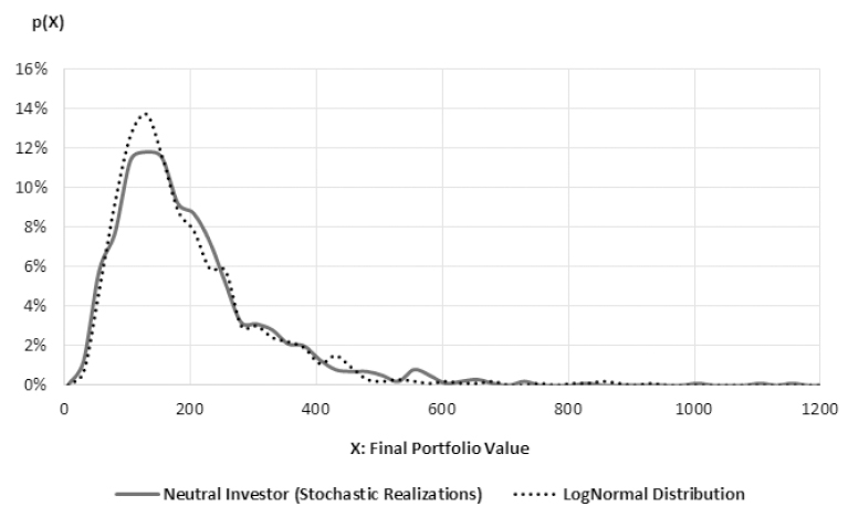
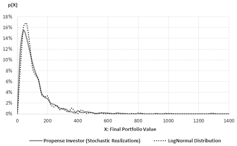
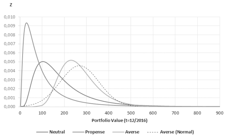
Figures 6, 7 and 8 show the probability density functions of portfolio values at the end of the simulation, based on 1,000 stochastic realizations of each agent type. The figures contain both experimental realizations and the theoretical approximation of distributions. Observations are log-normally distributed, avoiding negative values for the portfolio value. The log-normal distributions are a transformation of the original random variable final portfolio performance that are assumed to be normally distributed ($Y=ln\left(X\right)$). Location and scale parameters (μ, σ) for averse, neutral and risk-seeking investors are, respectively, (5.54, 0.32), (5.03, 0.63) and (4.26, 0.94). Figure 9 presents log-normal curves, and also the normal curve for risk-averse distributions, that also showed a good fit.

Figure 6:
Risk-averse investor’s probability density function. The distribution reflects 1,000 stochastic portfolio realizations for the risk-averse investor (first stage simulation).

Figure 7:
Risk-neutral investor’s probability density function. The distribution reflects 1,000 stochastic portfolio realizations for the risk-neutral investor (first stage simulation).

Figure 8:
Risk-seeking investor’s probability density function. The distribution reflects 1,000 stochastic portfolio realizations for the risk-seeking investor (first stage simulation).

Figure 9:
Experimental probability distributions. The random variables are the mean portfolio values at t=12/2016, assumed to be normally distributed: Risk-averse ~ N (268, 87); Risk-neutral ~ N (187,131); Risk-seeking ~ N (110,132). The log-normal distributions are a transformation of the original variables.

Figure 10 shows, for a specific point of the simulation period, the security market line and the efficient frontier related to the environment state at $t=\text{Jan-}2008$, a few months before the great impacts of the subprime crisis. At that time, an investor with 50% of risky assets in his portfolio would have an expected return of 1.9% and a portfolio risk close to 3.3%, while an investor with 100% of risk-free asset would have a return of 0.88%. The increasing expected return for risk-neutral investor in relation to risk-averse portfolio is around 1%, nonetheless the increasing in risk is about 3.3%. The same applies to risk-seeking investor, who would increase its expected return to 3.9%, facing a greater risk of 9.93%.

Figure 10:
Portfolios expected return (μ) and risk (σ). The figure shows the trade-off values for three agents randomly chosen at t=01/2008.

Table 2 presents the simulation data summary of first stage simulation. The maximum portfolio value among all simulated was $1,510.70, meaning a return of 1,410% in the period. A risk-seeking investor achieved it. Despite of that, the poorer performance regarding the 1º percentile of portfolio returns was also from the investor who faces the greater risk exposure. Comparing to an inflation-benchmarked portfolio ($187.26 at $t=01/2017$), 840 out of 1,000 risk-averse portfolio realizations were above this benchmark.

Table 2:
First stage simulation summary. There were 1,000 instances of each agent type. Portfolio values are at t= Jan-2017, considering zero transactions costs and matching demand and supply of stocks in capital market. Inflation-benchmarked portfolio reflects the inflation index (IPCA) of a $100.00 portfolio at t= Jan-2006. At the end of simulation, this portfolio performance was worth $187.26.

Agent Type	Portfolio Performance		Median	Max.	Mean percentile	Mean percentile	Performance Above Inflation (cases)
	μ	σ
AgT - Risk-Averse	267.89	87.43	256.20	830.26	623.66	101.00	84%
AgT - Risk-Neutral	187.12	130.89	156.13	1,265.71	869.39	21.39	38%
AgT - Risk-Seeking	110.11	131.52	71.69	1,510.70	939.78	1.59	15%

Figure 11 brings the results of each agent rationality driving his portfolio selection. It is notable the effect of the 2007/8 financial crisis in all of the agents’ portfolios, with a minor impact for the most conservative risk attitude. From $t=01/2006$ to $t=06/2008$ , risk-seeking agent had the best performance, reaching almost 114% of return in the period. The volatility of his returns continues after the deep falling prices at $t=12/2008$, when all of his past accumulated return disappeared. After twelve months ($t=12/2009$), the risk-seeking agent recovered his portfolio value and then started a descendent trend until the end of the simulation, with a negative accumulated return until $t=07/2016$.

Figure 11:
Portfolio performance history. It shows mean performances of initial R$ 100.00 portfolio value (BRL-Brazilian Real) of each one of the 3,000 agents. Bovespa Index reflects the Brazilian Stock Exchange index along simulation period, and inflation line brings an inflation-benchmarked portfolio.

Almost the same movements apply to the risk-neutral investor. The correlation between this agent type and the risk-seeking was 0.68 (Table 3). From $t=12/2008$ to the end of simulation, risk-averse had a better performance than risk-seeking investor did. At $t=01/2017$, his mean portfolio value was $187.12, very approximated to inflation-benchmarked portfolio and to IBOVESPA index. Actually, the correlation between risk-neutral performance and stock exchange index was 0.93, showing that random selected market portfolios (compound of only six assets) along the simulation period were a good proxy to the most common used market portfolio.

Table 3:
Correlations of mean portfolio returns. Measures are related to vector AgT_{1 x 3} = Risk-averse, Risk-neutral, Risk-seeking.

Investors	ρij
AgT1, AgT2	0.60
AgT1, AgT3	-0.17
AgT2, AgT3	0.68

Regarding risk-averse rationality, Figure 11 shows less accentuated variations in this portfolio value along the simulation history. The risk-averse investor have won the second half of the period, with a fixed weight of 50% risk-free asset, whereas risk-neutral invested exclusively in the market portfolio, and risk-seeking had a short position of 50% in risk-free asset. This suggests that a more conservative risk attitude would have been the optimal approach to wealth management in the context of the analyzed data.

The correlations between portfolio values along simulation period are in Table 3. It shows positive correlation between performance of the agents 1 and 2, and 2 and 3, while the performance of risk-averse and risk-seeking agents has a low negative correlation.

Figure 12 plots de average portfolio returns from the different starting points (periods) of the investments. The highest return in the period was over 150% for a risk-averse portfolio, starting in 2006 and maintained until the end of the simulation, while a risk-seeking portfolio would have obtained a negative average return of 50% if started in the middle of 2008. A return above 100% is observed for a risk-seeking portfolio started at the beginning of 2016, doubling the money invested in about 12 months. Considering the possible portfolio start-up periods within the simulation range, the average return of risk-averse portfolios stands out as long-term investment options.

Figure 12:
Portfolio performance history, by period of entry. The average return corresponds to the performances considering the different possible starting points of the investments.

4.2 Second stage: adaptive agents

In this stage, agents have adaptive behavior, and therefore can move along the security market line, with starting points set as in the first stage for each element of AgI _1000×3. The parameters of each agent are those of the first stage. Robustness checks in the second stage simulation are twofold.

Firstly, agents can increase their risk appetite, with minimum weight equal to the respective agent type: risk-averse agents can choose to invest 50% or more in market portfolio, risk-neutral can borrow at risk-free rate and reinvest this amount in market portfolio, and risk-seeking agent is flexible to be more than 50% short in CDI asset. The logic that drives this agent reasoning is the current portfolio excess return vis-à-vis the inflation-benchmarked portfolio. If the difference is positive, this gain will be reinvested in the capital market.

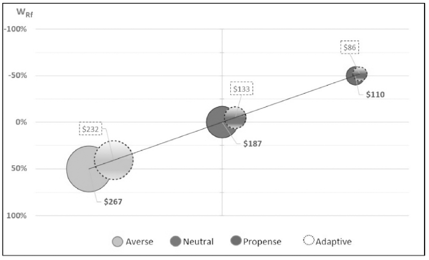
Simulation results are in Figure 13, showing that portfolio final values, compared to first stage simulation, lost value at $t=01/2017$ (-13%, -29% and -21%, respectively). Similarly, by allowing adaptive investor to decrease the α proportion of portfolio (Algorithm 4 in section 3.2) the wealth increased, respectively, in 15%, 53% and 33% (Fig. 14).

Figure 13:
Increasing Risk Appetite. Adaptive agents (risk-averse, risk-neutral and risk-seeking types) reinvest the portfolio excess return (vis-à-vis the inflation-benchmarked portfolio) in capital market by the rebalance event. Portfolio values at W _Rf = 50%, 0%, and -50% are those achieved in the first stage simulation.

Figure 14:
Decreasing Risk Appetite. Adaptive agents (risk-averse, risk-neutral and risk-seeking types) reinvest the portfolio excess return (vis-à-vis the inflation-benchmarked portfolio) in money market by the rebalance event. Portfolio values at W _Rf = 50%, 0%, and -50% are those achieved in the first stage simulation.

These results corroborate those of the first simulation, regarding the negative relation between increasing risk appetite and investor performance.

4.3 Hypothesis test and conjecture assessment

Hypothesis tests applied to portfolio performances in the simulation period ($t=01/2006$ to $t=01/2017$) showed that, considering the stochastic process conducted in the first stage simulation, cumulative mean returns of agents’ portfolios are statistically different at 1% significance level (Table 4). It is also interesting to note that the only period where returns are in a crescent order, in a way that they correspond to the associated crescent risk exposure, is before subprime crisis.

Table 4:
Hypothesis test. Tests are based on Sharpe performance measures - Equations 11 to 13 (^{Jobson & Korkie, 1981}). Comparisons are between types 1 and 2, and types 1 and 3 of vector AgT _{1 x 3} = Risk-averse, Risk-neutral, Risk-seeking.

Periods	${\mu }_{AgT=1}$	${\sigma }_{AgT=1}$				Results
	${\mu }_{AgT=2}$	${\sigma }_{AgT=2}$	${\widehat{Sh}}_{\mathrm{1,2}}$	Z1, 2	p-value1, 2
	${\mu }_{AgT=3}$	${\sigma }_{AgT=3}$	${\widehat{Sh}}_{\mathrm{1,3}}$	Z1, 3	p-value1, 3
01/2006-06/2008	60%	16%
	87%	33%	0.06	2.15	0.032**	Rejects H 0
	116%	52%	0.12	2.95	0.003***	Rejects H 0
07/2008-12/2010	26%	22%
	18%	45%	0.08	2.75	0.006***	Rejects H 0
	2%	72%	0.18	3.89	0.000***	Rejects H 0
01/2011-06/2013	4%	25%
	-16%	51%	0.06	1.73	0.084*	Do Not Rejects H 0
	-33%	82%	0.11	2.07	0.038**	Rejects H 0
07/2013-01/2017	40%	28%
	24%	56%	0.156	3.88	0.000***	Rejects H 0
	3%	89%	0.347	5.23	0.000***	Rejects H 0
2006-2017 (full period)	168%	32%
	87%	65%	0.81	12.50	0.000***	Rejects H 0
	10%	106%	1.74	15.12	0.000***	Rejects H 0

• Notes: Significance levels are 1% (***), 5%(**) and 10%(*). The null hypothesis is that performances are equivalent.

Consequently, we can reject the null hypothesis in favor of the alternative statement: (H1 _a) Risk-averse investors, who select lower associated risk and expected return portfolios than risk-seeking investors, have better comparative performance, using a common market portfolio.

Therefore, restricted to the studied country level, our research conjecture finds support in the designed bottom-up approach, which has sown that the optimal behaviors would be those less oriented towards risk. Furthermore, especially in upward trends of sovereign debt risk premium, rational choices of portfolio selection, with the assumption of risk-free asset availability, can build a trigger to the critical sovereign debt cycle in consequence of the debt dynamics that reflects economic growth and interest rate levels.

Figure 15 shows the treasury liabilities and the respective market perception of risk measured by the Emergent Markets Bond Index Plus for Brazilian external debt (EMBI+Br). The graph illustrates a negative correlation (-0.72) between EMBI+Br and the risk-seeking simulated portfolios, denoting that negative feedbacks of sovereign spreads in the doom-loop dynamics, beyond affecting government securities prices, have loss impact for risk-seeking investors, albeit debt overhang could undermine both strategies. In the long run, the propensity to save and to postpone investments may reveal a fragility regarding the availability of the relatively risk-free assets.

Figure 15:
National treasury issued bonds and risk index (EMBI+Br). The graph shows a negative correlation pattern between risk-seeking simulated portfolios and the sovereign risk index. Despite the two peaks (2007/8 financial crisis, and political crisis of country president’s impeachment), the mean spread over US Treasury is around 252 basis points in the period, a reasonable low measure of default or liquidity risks. The existence of peaks in the EMBI+Br and its volatility could challenge a strict sense definition of risk-free asset in emerging economies, though.

Therefore, sound debt burden indicators, interest rate levels, inflation, economic growth, and public budget targets are critical components of policies for sustainable debt dynamics. In a low - or even negative - interest rate environment, which challenges advanced economies around the world in the aftermath of the global financial crisis (^{Rogoff, 2017}), fomenting entrepreneurial investments into projects demands reasonable expected payouts vis-à-vis risk-free asset benchmarks.

Complementary, sound political and legal institutions can also influence risk behavior, stimulating higher risk-taking by banks as shown in ^{Ashraf (2017}). According to ^{Levine, Lin, and Xie (2016}), the development of capital market act as a “spare tire” during banking crises, providing alternative corporate financial channel and mitigating the economic severity of those crises. However, risk-taking behavior could generate moral hazard problems because of government bailout expectations - one of the propagation channels in the doom-loop of the sovereign debt.

The Brazilian capital market has 338 listed companies, a market equity around USD 841 billion, with a ratio of 0.89 to the national public debt outstanding. The volume of traded stocks in May-2017 had participation of domestic financial institutions (6%) and foreign investors (52%), among others (^{BM&FBOVESPA, 2017}). Strengthen legal institutions to improve business confidence levels could help to rebalance investors’ risk appetite and to reduce the likelihood of a sovereign debt doom-loop.

Regarding the research question, the study has shown that rational behavior can lead to systemic risk situations. Even though it was a simulation procedure with relevant constraints to the financial markets reality and to the investment options, the experiment allows including one of the main functions of a bond - which is to provide a liquidity source to the investors - as a potential trigger to the critical sovereign debt cycle. In a pre-doom-loop situation, the level of public debt to GDP could difficult government bond issues to supply rational investors demand or to accomplish monetary policy goals. This condition could affect the market perception of bonds risk and initiate sovereign downgrades that starts the doom-loop. Furthermore, cascade events might imply bank defaults and systemic risk concerns.

5 CONCLUSION AND FUTURE WORK

The scarcity of safe assets is challenging economies around the world, as in the European Union, where banks hold € 1.9 trillion of euro sovereign bonds. On the other hand, investment in sovereing securites creates a potent doom-loop between sovereign risk and investor risk, which can spread financial systemic risk. Besides being a liquid font of cash, the usefulness of safe assets is also related to regulatory capital requirements to financial institutions that follows Basel prudential criteria, as a zero weight financial instrument.

Using a bottom-up approach and Brazilian financial market data from 2006 to 2017, this study has examined the rationality of three types of agents, regarding their risk attitude that drives portfolio selection decision. Among the risk attitudes, the risk-averse agent, who invested half or his wealth in risk-free assets like sovereign bonds, has reached the most successful rationality. The results were obtained by two stages of stochastic simulations using 3,000 agents instances, which showed log-normally probability density functions for the three agent types. We considered zero transactions costs and matching demand and supply in the capital market.

The results - limited to the context studied reflecting the country data of the sample and therefore without the generalization attribute - have confirmed our hypothesis that risk-averse investors, acting rationally in order to manage their asset portfolios, can be seen as a potential trigger to the doom-loop that connects sovereign and bank risks (^{Brunnermeier et al., 2016}). The demand for sovereign bonds feeds the cyclical problem, and the initial economic shock that would affect the sovereign risk should also be viewed as an endogenous factor, the debt dynamics itself. This brings significant issues to policymakers in charge of financial system regulation, to fiscal and public budget constraints, and to the development of capital markets. Growing ratios of sovereign debt to GDP place an additional concern to debt overhang.

As main shortcomings of the study, the market portfolio should incorporate assets from other markets beyond the stock market to better diversification achievement. Besides this, we can add the myopic characteristic of the agents in managing their portfolios and the absence of the fundamentalist analysis skills to the agents.

Regarding the agent-based methodology, the process of programming, testing and executing the software components of the model may be time-consuming, especially when the framework is at early development stages. Despite this, it can also be worth building or extending a framework to promote new research questions.

Future studies could deal with corporate governance actors - important agents to the credibility of stock markets - in order to cope with the classical principal-agent problem. Debt dynamics analysis could also incorporate forward-looking paths simulations with variables like economic growth and interest level. Different approaches to portfolio selection could be implemented, as the use of itemsets (^{Baralis et al., 2017}), evolutionary algorithms (^{Macedo et al., 2017}) or stochastic dominance strategies (^{Bruni et al., 2017}).

ACKNOWLEDGEMENTS

We thank conference anonymous referees for very helpful comments on earlier drafts. The first author would like to acknowledge the Central Bank of Brazil, and register that the views expressed in the study are exclusively those of the authors, and not necessarily from the mentioned institution nor from its members.

REFERENCES

• ¹
  ACHARYA V & RAJAN RG. 2013. Sovereign Debt, Government Myopia, and the Financial Sector. The Review of Financial Studies, 26(6): 1526-1560.
• ²
  ALLEN F & CARLETTI A. 2013. What is Systemic Risk? Journal of Money, Credit and Banking, 45(1): 121-127.
• ³
  ALTAVILLA C, PAGANO M & SIMONELLI S. 2016. Bank exposures and sovereign stress transmission. European Systemic Risk Board, Working Paper n. 11.
• ⁴
  ASHRAF BN. 2017. Political institutions and bank risk-taking behavior. Journal of Financial Stability, 29: 13-35.
• ⁵
  ASHRAF Q, GERSHMAN B & HOWITT P. 2017. Banks, market organization, and macroeconomic performance: An agent-based computational analysis. Journal of Economic Behavior & Organization, 135: 143-180.
• ⁶
  BARALIS E, CAGLIERO L & GARZA P. 2017. Planning stock portfolios by means of weighted frequent itemsets. Expert Systems with Applications, 86: 1-17.
• ⁷
  BERUTICH JM, LÓPEZ F, LUNA F & QUINTANA D. 2016. Robust technical trading strategies using GP for algorithmic portfolio selection. Expert Systems with Applications, 46: 307-315.
• ⁸
  BLACK L, CORREA R, HUANG C & ZHOU H. 2016. The systemic risk of European banks during the financial and sovereign debt crises. Journal of Banking and Finance, 63: 107-125.
• ⁹
  BM&FBOVESPA - BRAZILIAN STOCK EXCHANGE. 2017. http://www.bmfbovespa.com.br/ Accessed 10.06.2017.
  » http://www.bmfbovespa.com.br/
• ¹⁰
  BOWDLER C & ESTEVES RP. 2013. Sovereign debt: the assessment. Oxford Review of Economic Policy, 29(3): 463-477.
• ¹¹
  BRUNI R, CESARONE F, SCOZZARI F & TARDELLA F. 2017. On exact and approximate stochastic dominance strategies for portfolio selection. European Journal of Operational Research, 259: 322-329.
• ¹²
  BRUNNERMEIER MK, GARICANO L, LANE P, PAGANO M, REIS R, SANTOS T, THESMAR D, VAN NIEUWERBURGH S & VAYANOS D. 2016. The sovereign-bank diabolic loop and ESBies. American Economic Review, 106(5): 508-512.
• ¹³
  CAMPBELL JY, LO W & MACKINLAY AC. 1997. The Econometrics of Financial Markets. New Jersey: Princeton University Press, (Chapter 5).
• ¹⁴
  CUI B, WANG H, YE K & YAN J. 2012. Intelligent agent-assisted adaptive order simulation system in the artificial stock market. Expert Systems with Applications, 39: 8890-8898.
• ¹⁵
  DONADELLI M & PERSHA L. 2014. Understanding Emerging Market Equity Risk Premia: Industries, Governance and Macroeconomic Policy Uncertainty. Research in International Business and Finance, 30: 284-309.
• ¹⁶
  DOSI G, FAGIOLO G, NAPOLETANO M, ROVENTINI A & TREIBICH T. 2015. Fiscal and monetary policies in complex evolving economies. Journal of Economic Dynamics & Control, 52: 166-189.
• ¹⁷
  ECB - EUROPEAN CENTRAL BANK. 2010. Recent Advances in Modelling Systemic Risk Using Network Analysis. http://www.ecb.europa.eu/ Accessed 07.11.2013.
  » http://www.ecb.europa.eu/
• ¹⁸
  ESRB - EUROPEAN SYSTEMIC RISK BOARD. 2015. Report on the regulatory treatment of sovereign exposures. http://www.esrb.europa.eu/ Accessed 05.11.2016.
  » http://www.esrb.europa.eu/
• ¹⁹
  FELDMAN T. 2010. Portfolio manager behavior and global financial crises. Journal of Economic Behavior & Organization, 75: 192-202.
• ²⁰
  FERREIRA RJP, ALMEIDA FILHO AT & SOUZA FMC. 2009. A decision model for portfolio selection. Pesquisa Operacional, 29(2): 403-417.
• ²¹
  GARTNER IR. 2012. Differentiated risk models in portfolio optimization: a comparative analysis of the degree of diversification and performance in the São Paulo Stock Exchange (BOVESPA). Pesquisa Operacional, 32(2): 271-292.
• ²²
  GE J. 2017. Endogenous rise and collapse of housing price - An agent-based model of the housing market. Computers, Environment and Urban Systems, 62: 182-198.
• ²³
  GIBSON HD, HALL SG & TAVLAS GS. 2017. Self-fulfilling dynamics: The interactions of sovereign spreads, sovereign ratings and bank ratings during the euro financial crisis. Journal of International Money and Finance, 73: 371-385.
• ²⁴
  IMF - INTERNATIONAL MONETARY FUND. 2017. Debt Sustainability Analysis. http://www.imf.org/ Accessed 22.02.2017.
  » http://www.imf.org/
• ²⁵
  JOBSON JD & KORKIE BM. 1981. Performance Hypothesis Testing with the Sharpe and Treynor Measures. The Journal of Finance, 36(4): 889-908.
• ²⁶
  KO P & LIN P. 2008. Resource allocation neural network in portfolio selection. Expert Systems with Applications, 35: 330-337.
• ²⁷
  KOLM PN, TUTUNCU R & FABOZZI FJ. 2014. 60 Years of portfolio optimization: Practical challenges and current trends. European Journal of Operational Research, 234: 356-371.
• ²⁸
  LAEVEN L & VALENCIA F. 2013. Systemic Banking Crises Database. IMF Economic Review, 61(2): 225-270.
• ²⁹
  LEVINE R, LIN C & XIE W. 2016. Spare tire? Stock markets, banking crises, and economic recoveries. Journal of Financial Economics, 120: 81-101.
• ³⁰
  LINTNER J. 1965. The Valuation of Risk Assets and the Selection of Risky Investments in Stock Portfolios and Capital Budgets. The Review of Economics and Statistics, 47(1): 13-37.
• ³¹
  LIU S. 2011. A fuzzy modeling for fuzzy portfolio optimization. Expert Systems with Applications, 38: 13803-13809.
• ³²
  MACEDO LL, GODINHO P & ALVES MJ. 2017. Mean-semivariance portfolio optimization with multiobjective evolutionary algorithms and technical analysis rules. Expert Systems with Applications, 79: 33-43.
• ³³
  MARKOWITZ H. 1952. Portfolio Selection. The Journal of Finance, 7(1): 77-91.
• ³⁴
  MEHRA R & PRESCOTT EC. 1985. The Equity Premium - A Puzzle. Journal of Monetary Economics, 15: 145-161.
• ³⁵
  REINHART CM & ROGOFF KS. 2011. From Financial Crash to Debt Crisis. American Economic Review, 101(5): 1676-1706.
• ³⁶
  REKIK YM, HACHICHA W & BOUJELBENE Y. 2014. Agent-Based Modeling and Investors’ Behavior Explanation of Asset Price Dynamics on Artificial Financial Markets. Procedia Economics and Finance, 13: 30-46.
• ³⁷
  RODDER W, GARTNER IR & RUDOLPH S. 2010. An entropy-driven expert system shell applied to portfolio selection. Expert Systems with Applications, 37: 7509-7520.
• ³⁸
  ROGOFF K. 2017. Monetary policy in a low interest rate world. Journal of Policy Modeling, in press.
• ³⁹
  SHARPE WF. 1964. A Theory of Market Equilibrium under Conditions of Risk. The Journal of Finance, 19(3): 425-442.
• ⁴⁰
  SHOHAM Y & LEYTON-BROWN K. 2009. Multiagent Systems: Algorithmic, Game-Theoretic, and Logical Foundations. New York: Cambridge University Press, (Chapter 10).
• ⁴¹
  SILVA W, KIMURA H & SOBREIRO VA. 2017. An analysis of the literature on systemic financial risk: A survey. Journal of Financial Stability, 28: 91-114.
• ⁴²
  STN - SECRETARIA DO TESOURO NACIONAL (BRAZILIAN NATIONAL TREASURY). 2016. Relatório Mensal da Dívida Pública Federal - Setembro, 2016. http://www.tesouro.fazenda.gov.br/ Accessed 12.11.2016.
  » http://www.tesouro.fazenda.gov.br/
• ⁴³
  WOOLDRIDGE M. 2009. An Introduction to Multiagent Systems. West Sussex: John Wiley & Sons Ltd.

• *
  A preliminary version of this study was published in the book “Multi-Agent Based Simulation XVIII”, by Springer (2018).

Publication Dates

• Publication in this collection
  09 May 2019
• Date of issue
  Jan-Apr 2019

History

• Received
  20 Oct 2017
• Accepted
  07 Nov 2018