INTEGRATED LOTSIZING, SCHEDULING AND BLENDING DECISIONS IN THE SPINNING INDUSTRY

ABSTRACT

In this paper, the relevance of integrated planning concerning decisions of production and blending in a spinning industry is studied. The scenario regards a plant that produces several yarn packages over a planning horizon. Each yarn type is produced using a blend of several cotton bales that must contain attributes to ensure the quality of the produced yarns. Three approaches to managing production and blending are compared; the first deals with the solution to the production scheduling and blending problems in a single integrated model. The second approach hierarchically addresses these problems. The third procedure combines features from the integrated and hierarchical approaches. These approaches are applied to a real-world problem, and their respective performances are analyzed. The third approach proved to deal with lot sizing, scheduling and blending in the spinning industry more efficiently. Moreover, the results indicate the importance of coordinating production and blending decisions.

Keywords:
production planning; lotsizing and scheduling problem; blending problem; spinning industry

1 INTRODUCTION

The production planning problem in the spinning industry must determine the size and sequence of yarn production lots as well as which cotton bales will provide a fiber blend that ensures quality attributes to produce required yarns. These decisions involve lotsizing, scheduling and blending problems. The lotsizing and scheduling problem determines the timing, level and sequence of production to meet yarn demand over a time horizon. In order to represent the production environment, constraints related to setup, inventory and capacity must be respected. The blending problem determines the number of cotton bales used in each blend to feed the spinning machine. These problems arise in a two-stage production system in which the fiber blend is produced at the first stage (opening-blending machine) and the yarns are produced at the second stage on various spinning machines. There is a quality relationship between the first and second stages. The yarns have attribute specifications that can be achieved by an appropriate blend of fibers (^{El Mogahzy, 2004}). The specifications are related to the fiber attributes, such as grade color, trash percentage area, fiber length and others. Each blend must be composed by a given number of cotton bales in which the fibers ensure the specifications of the yarn requirements. The yarns belong to product families that differ in their attributes. Two blend loads for the same yarn family should have a minimal difference regarding their attributes. On contrary, yarns can present different unwanted features, causing production problems at the next level of the textile supply chain. Clearly, these constraints show the dependence of the raw cotton blend on the yarn production. ^{Crama et al. (2001}) also pointed out the utmost importance of dealing with the raw material in the production planning of process industries.

In the past, as pointed out by ^{Hax & Meal (1973}), the study of production problems solved hierarchically was justified by the data processing incapability of dealing with the optimization of the entire system. Planners also used to draw the production plan hierarchically. Even today, hierarchical decisions are supported by issues such as a decision-making process involving various levels of management and discordant planning horizons. Even though the sequential improvement procedures can theoretically converge the hierarchical decisions to an optimum final plan, this approach requires significant computational efforts. Furthermore, some broader objectives could only be perceived by approaching a detailed integrated model of the production process. This is true in the presence of high interaction among problems, as happens in the spinning industry dealing with production-scheduling and blending decisions.

The integrated lotsizing and scheduling problem has received attention in the literature due to its relevance to real-world problems. Tackling both problems simultaneously allows for better production plans than those obtained from a hierarchical planning system in which lot sizing is decided a priori and provides inputs to the scheduling level. Reviews summarizing research on this subject are presented in ^{Drexl & Kimms (1997}), ^{Kallrath (2002}), ^{Zhu & Wilhelm (2006}), ^{Copil et al. (2017}) and ^{Wörbelauer et al. (2019}). Moreover, some examples of lotsizing and scheduling studies in process industries are those of ^{Kopanos et al. (2010}) (yogurt production), ^{Toscano et al. (2019}) (beverage industry), ^{Claassen et al. (2016}) (food industry) and ^{Camargo et al. (2014}) (spinning industry).

In practice, lot sizing and scheduling, and blending in the spinning industry are hierarchically determined. First, lotsizing and scheduling decisions are taken. Then, the blend is defined, load after load, to meet the quality specifications. This strategy can be considered myopic, as it does not take into account attribute variations in the stored bales that can influence future blending decisions, and impact (and constrain) the subsequent plans. In other words, the production plan defined by the traditional hierarchical approach is not executed if the needed set of cotton bales for the blend is not available. Integrating the production-blending problem aims to draw up a production plan which has better control concerning attribute variations.

Three approaches to manage these operations are compared in this paper: one in which the production-scheduling and blending problems are solved within a single model, another in which they are solved separately (in a hierarchical way), and the last is a partial integrated approach. Our integrated model attempts to simultaneously define the production schedule and the selection of cotton bales. In the hierarchical design, the production plan is determined a priori. Then, the cotton bales for each blend load are chosen. Regarding the partial integrated approach, it first solves the production schedule, as well as a few blending constraints, and the cotton bales are then selected in a second step.

This paper aims to show that production planning must contemplate blending constraints in the decision-making process using mathematical models. This implication is shown by comparing the production and blending plans given by the integrated and hierarchical approaches. This comparison is built on an instance drawn from a spinning real-world problem. Also, this work provides three mathematical approaches to assist decision-makers in systemic production and blending planning.

The next section provides a background to the problem appearing in the spinning industry. The integrated lot sizing, scheduling and blending is defined in Section 3. The developed integrated model is also shown there. An analysis to compare the integrated and hierarchical approaches is reported in Section 4. Section 5 introduces the partial integrated approach that includes features from the integrated and hierarchical ones. Final remarks and suggestions of future work are addressed in Section 6.

2 THE SPINNING INDUSTRY

A spinning plant can produce different types of yarns with specifications that are determined by the customers. Failure to meet yarn specifications causes customer dissatisfaction, a decrease in the price of the product and a loss of production efficiency. The success of a spinning operation can be measured by the quality of the produced yarns and the manufacturing costs, and therefore both criteria help to determine the competitiveness of a company. The yarn manufacturing costs are measured by the raw material and production process costs. According to ^{Admuthe & Apte (2009}), raw material costs can represent up to 70 percent of the yarn price.

In an open-end spinning business, as studied in this paper, raw cotton is purchased in bales. The production flow to transform the raw cotton to yarns is depicted in Figure 1. From beginning to end, the fibers are processed on four machine groups. First, the cotton bales are opened, and the lint blended. The second step is to clean and blend the cotton lint. The third group of machines aligns and draws the fibers carding to make a long bundle called sliver. Lastly, various spinning machines draw and twist the sliver to make the yarn. It is wound around bobbins or tubes to be transported to the customers. In this spinning sequence, the two intermediate processes can work in a synchronized way with the opening and mixing processes. Therefore the production system consists of two stages, as illustrated in Figure 1.

Figure 1
Sequence of processes and stages in yarn production.

The production should be governed by a plan that informs the machine and the time by which each required yarn must be produced. While respecting the synchronization of stages, planning must provide information about the fiber blend, that is, which yarn family is to be produced by each blend load and its starting and finishing times. Once the blend sequence is known, the decision-maker must select the cotton bales to make up the fiber blend that ensures the specification for each yarn attribute. A mathematical model to represent this integrated lotsizing, scheduling and blending problem is discussed in the next section. ^{Cunha et al. (2018}) and ^{Pereira et al. (2020}) propose an analysis of decisions related to the raw material by the integration of raw material problems in the lot sizing (and scheduling) problem. However, we propose an approach focusing on the operational level of decisions.

3 INTEGRATING LOT SIZING, SCHEDULING AND BLENDING

This section proposes a mathematical model for the integrated lotsizing, scheduling and blending problem in the spinning industry. The problem solution draws up a production plan in which the blend loads are sequenced, and their required qualities are determined. Moreover, the yarn amount (and its sequence) is established to be produced on each machine complying with the blend quality. The other part of the plan must define the cotton bales selected to be ingredients of the blend loads. This planning aims to meet the required specifications for the yarns and should minimize production costs and the attribute variability between blends. The mathematical model presented below is an integration of the lotsizing and scheduling problem and the blending problem. The lotsizing and scheduling constraints are based on the multi-stage hybrid lotsizing and scheduling model proposed in ^{Camargo et al. (2012}). The blending constraints are compatible with some ideas from ^{Zago (2005}).

3.1 Definition of lotsizing and scheduling problem

A spinning mill can produce different types of yarns on several parallel machines. The production plan must define the production for each yarn in each period over a finite planning horizon. The demand for the yarns is known and should be met when capacity is sufficient. Delays can occur if the demand for yarns is high; therefore, backlogs must be represented in the model.

The production of a yarn in a given time period imposes the condition that a suitable fiber blend also be processed in that bucket. Thus the planning of the second stage requires the planning of the first stage. That is, with a blend load (first stage), it is possible to produce specific products (second stage). A blend load consists of a set of bales of a certain quality of fibers. The yarns belong to families related to the required blend and quality specifications. A fiber blend is generally used in several yarns, but a yarn is made of only one fiber blend. At each point in time, only one fiber blend can be processed by load on this kind of production line; thus, all the machines must produce yarns of the same family. It is possible to produce more than one family, but it requires the tracking of raw material and intermediate products. This industrial feature is not considered in the study.

Machines may differ in their processing rates of the same yarn, and consequently, the fiber blend can be consumed at different speeds. A setup changeover from one yarn to another consumes a capacity time dependent on the sequence in which the yarns are processed. This characteristic imposes scheduling constraints jointly formulated with lotsizing constraints. Setups can be carried from one period to the next. The setup changeover for a fiber blend can be considered null as another fiber blend is immediately available for later use in production.

The definition of the lotsizing and scheduling problem for the spinning industry can be represented by the following mathematical model, as proposed by ^{Camargo et al. (2014}). From the results shown, this model presented the best results for the problem. The model considers continuous time periods for the first stage. In the second stage, production slots are considered, representing production in a semi-continuous manner. The indices, parameters and decision variables for the lot sizing and scheduling are defined as follows:

Indices i = 1,..., N yarn types; k = 1,..., K yarn families - blend quality types; m = 1,..., M spinning machines; t,t'= 1,..., T periods; l = 1,..., L blend loads available within the planning horizon. Parameters c itt' cost of producing one kilogram of yarn i in period t to fulfill the demand of period t l ; σ mij setup cost of a changeover on machine m from yarn i to yarn j; r l cost of one kilogram of residue of the lth blend load; d it' demand (kilograms) of yarn i in period t l ; s mij fraction of a single period consumed for the production setup of a changeover on machine m from yarn i to yarn j; p mi fraction of a single period consumed for production on machine m, of one kilogram of yarn i; C opening-and-blending machine capacity (kilograms) for one blend load; S(k) yarn set belonging to the same family k. Variables X mitlt' production (kilograms) on machine m of yarn i in period t using the lth blend load to meet demand in period t l ; Y mijtl takes 1, if a changeover occurs on machine m from yarn i to j in period t using the lth blend load; 0 otherwise; R l raw cotton residue (kilograms) of the lth blend load; U lk takes 1, if the lth blend load satisfies the quality for yarn family k; 0 otherwise; u l s starting time of the lth blend load; u l f finishing time of the lth blend load; μ m i t l s production starting time on machine m of yarn i in period t using the lth blend load; μ m i t l f production finishing time on machine m of yarn i in period t using the lth blend load; α mitl takes 1, if machine m is set up for production of yarn i in period t using the lth blend load; 0 otherwise; P t l s takes 1, if the lth blend load starts before the end of period t (that is, instant time t); 0 otherwise; P t l f takes 1, if the lth blend load ends after the beginning of period t (that is, instant time t − 1); 0 otherwise.

Indices
i = 1,..., N	yarn types;
k = 1,..., K	yarn families - blend quality types;
m = 1,..., M	spinning machines;
t,t'= 1,..., T	periods;
l = 1,..., L	blend loads available within the planning horizon.
Parameters
c itt'	cost of producing one kilogram of yarn i in period t to fulfill the demand of period t l ;
σ mij	setup cost of a changeover on machine m from yarn i to yarn j;
r l	cost of one kilogram of residue of the lth blend load;
d it'	demand (kilograms) of yarn i in period t l ;
s mij	fraction of a single period consumed for the production setup of a changeover on machine m from yarn i to yarn j;
p mi	fraction of a single period consumed for production on machine m, of one kilogram of yarn i;
C	opening-and-blending machine capacity (kilograms) for one blend load;
S(k)	yarn set belonging to the same family k.
Variables
X mitlt'	production (kilograms) on machine m of yarn i in period t using the lth blend load to meet demand in period t l ;
Y mijtl	takes 1, if a changeover occurs on machine m from yarn i to j in period t using the lth blend load; 0 otherwise;
R l	raw cotton residue (kilograms) of the lth blend load;
U lk	takes 1, if the lth blend load satisfies the quality for yarn family k; 0 otherwise;
$u_l^s$	starting time of the lth blend load;
$u_l^f$	finishing time of the lth blend load;
${\mu }_{mitl}^s$	production starting time on machine m of yarn i in period t using the lth blend load;
${\mu }_{mitl}^f$	production finishing time on machine m of yarn i in period t using the lth blend load;
α mitl	takes 1, if machine m is set up for production of yarn i in period t using the lth blend load; 0 otherwise;
$P_{tl}^s$	takes 1, if the lth blend load starts before the end of period t (that is, instant time t); 0 otherwise;
$P_{tl}^f$	takes 1, if the lth blend load ends after the beginning of period t (that is, instant time t − 1); 0 otherwise.

$\mathbf{\text{Minimize}}\sum _{m=1}^M\sum _{i=1}^N\sum _{t=1}^{T+1}\sum _{l=1}^L\sum _{t\text{'}=1}^T{c}_{itt\text{'}}·X_{mitlt\text{'}}+\sum _{m=1}^M\sum _{i=1}^N\sum _{j=1}^N\sum _{t=1}^T\sum _{l=1}^L{\sigma }_{mij}·Y_{mijtl}+\sum _{l=1}^L{r}_l·R_l$ (1)

Subject to lotsizing and scheduling constraints:

$\sum _{k=1}^K{U}_{lk}\le 1\forall l$ (2)

$u_l^s\le u_l^f\le T\forall l$ (3)

$u_l^f=u_{\left(l+1\right)}^s\forall l<L$ (4)

$\sum _{m=1}^M\sum _{t=1}^{T+1}\sum _{l=1}^L{X}_{mitlt\text{'}}=d_{it\text{'}}\forall i,t\text{'}$ (5)

${\mu }_{mitl}^f-{\mu }_{mitl}^s\ge \sum _{j=1}^N\left(s_{mji}·Y_{mjitl}\right)+p_{mi}·\sum _{t\text{'}=1}^T{X}_{mitlt\text{'}}\forall m,i,t,l$ (6)

$\sum _{i=1}^N\sum _{l=1}^L\left({\mu }_{mitl}^f-{\mu }_{mitl}^s\right)\le 1\forall m,t$ (7)

${\mu }_{mitl}^s\ge {\mu }_{mjtl}^f+Y_{mjitl}-1\forall m,i,j,t,l$ (8)

$\sum _{t\text{'}=1}^T{p}_{mi}·X_{mitlt\text{'}}\le \sum _{j=1}^N{Y}_{mjitl}+{\alpha }_{mitl}\forall m,i,t,l$ (9)

$\sum _{j=1}^N{Y}_{mjitl}+{\alpha }_{mitl}=\sum _{j=1}^N{Y}_{mijtl}+{\alpha }_{mit\left(l+1\right)}\forall m,i,t,l<L$ (10)

$\sum _{j=1}^N{Y}_{mjitL}+{\alpha }_{mitL}=\sum _{j=1}^N{Y}_{mijtL}+{\beta }_{mi\left(t+1\right)1}\forall m,i,t$ (11)

$\sum _{i=1}^N{\alpha }_{mitl}=1\forall m,t,l$ (12)

$\sum _{j=1}^N{Y}_{mjitl}\le 1\forall m,i,t,l$ (13)

$\sum _{m=1}^M\sum _{i=1}^N\sum _{t=1}^T\sum _{t\text{'}=1}^T{X}_{mitlt\text{'}}+R_l=C·\sum _{k=1}^K{U}_{lk}\forall l$ (14)

$$\begin{gathered} X_{mitlt\text{'}}\le d_{it\text{'}}·U_{lk}\forall m,i\in S\left(k\right) \\ \forall t,l,t\text{'},k \end{gathered}$$ (15)

$\sum _{t=1}^T\sum _{i=1}^N\left({\mu }_{mitl}^f-{\mu }_{mitl}^s\right)\le u_l^f-u_l^s\forall m,l$ (16)

${\mu }_{mitl}^f-T·\left(P_{tl}^s+P_{tl}^f-1\right)\le {\mu }_{mitl}^s\le {\mu }_{mitl}^f+T·\left(P_{tl}^s+P_{tl}^f-1\right)\forall m,i,t,l$ (17)

$max\left(t-1;u_l^s-T·\left(1-P_{tl}^s\right)\right)\le {\mu }_{mitl}^s\le min\left(t;u_l^f+T·\left(1-P_{tl}^f\right)\right)\forall m,i,t,l$ (18)

$max\left(t-1;u_l^s-T·\left(1-P_{tl}^s\right)\right)\le {\mu }_{mitl}^f\le min\left(t;u_l^f+T·\left(1-P_{tl}^f\right)\right)\forall m,i,t,l$ (19)

$Y_{mijtl}\in \left\{0,1\right\};U_{lk}\in \left\{0,1\right\};P_{tl}^s\in \left\{0,1\right\};P_{tl}^f\in \left\{0,1\right\}\forall m,i,j,t,l,k$ (20)

$\text{all other variables are non-negative and continuous.}$ (21)

The objective function (1) relates to the lot sizing and scheduling and aims to minimize the costs of backlogging, inventory, changeover and residue. Here, the amount produced before the delivery date is considered as inventory, given by X _mitlt' when $t<t\text{'}$. On the other hand, X _mitlt' for $t>t\text{'}$ is the amount produced after the delivery date, that is, backlogged orders. Similarly, the production costs c _itt' refer to holding costs when $t<t\text{'}$ and to backlog costs when $t>t\text{'}$. For $t=t\text{'}$, c _itt' equals zero, as the production of period t meets the demand of the same period. Note that to accommodate the unfulfilled demand at the end of the planning horizon, a dummy period is also considered in the objective function. The constraint group (2)-(4) defines the schedule of the blend loads. Each blend load is constrained according to constraints (2) to meet the requirements for at most one yarn family. Constraints (3) and (4) avoid the overlapping of the starting and finishing blend loads. Note that a blend allocation to a load is allowed without production. Naturally, it generates residues that are detected in the second-stage requirements. Constraints (5)-(13) define the second-stage production system. Equations (5) attempt to satisfy the demand by taking into account inventories and backlogging. Requirements (6) establish the time used to set up the machine and to produce each yarn. Observe that, together with (7), the production slots are confined to a period of size one. The confinement is made by normalizing X _mitt' with p _mi . Similarly, s _mji refers to the fraction of the period wasted in setting up machine m. Constraints (6) and (7) allow for machine idle times in and between slots. Constraints (8) define the production slot sequences and avoid sub tour in the sequence. The flow of the machine setup is ensured by (9)-(13). The production is ensured (9) by setting up the machine or carrying a previous configuration over periods or blends. The setup carried over blend loads and periods is represented in (10) and (11), respectively. Constraints (12) ensure that each machine is set up for the production of one yarn in each period. Constraints (13) limit one yarn type to changeover to one in each production slot. The constraint group (14)-(19) integrates the first-and second-stage constraints. Constraints (14) define the all-or-nothing production for the blending machine. Specifically, the total amount of the blend is used either as production or as residue (Remark (2) presents a case in which the residue must completely used). Requirements (15) allow for yarn production that belongs to the family of the blend load in case it exists. Constraints (16)-(19) define the useful production slots, that is, when $P_{tl}^s=P_{tl}^f=1$. Let $P_{tl}^s=1$ if the lth blend load starts before the end of period t (i.e. at instant t), $P_{tl}^s=0$ otherwise. Further, $P_{tl}^f=1$ if the availability of the lth blend load ends after the beginning of period t (i.e. at instant t − 1), $P_{tl}^f=0$ otherwise. Figure 2 provides some examples of the variables $P_{tl}^s$ and $P_{tl}^f$. In cases 2.a, 2.b and 2.c, the blend load starts before the end of period $t\left(P_{tl}^s=1\right)$. In cases 2.a, 2.b and 2.d, the blend load finishes after the beginning of period $t\left(P_{tl}^f=1\right)$. Constraints (17) are active when $P_{tl}^s=0$ or $P_{tl}^f=0$. In this case, the lth blend load does not occur in period t and ${\mu }_{mitl}^s={\mu }_{mitl}^f$, forbidding production in that slot. Constraints (18)-(19) define lower bounds on the production slot starting time, when $P_{tl}^s=1$, and upper bounds on the slot ending time, when $P_{tl}^f=1$.

Figure 2
Illustrative examples for the P ^s and P ^f concept.

3.2 Definition of blending problem

The blending problem is defined by ^{El Mogahzy (2004}) and ^{El Mogahzy et al. (2004}) as the process of combining different fiber attributes to achieve a homogeneous blend. Its importance is emphasized by a fiber statistical analysis in (^{El Mogahzy, 2004}) that testifies the attributes which affect the yarn specifications. One of the most common spinning problems that often results from high variability of attributes between blends is the so-called fabric barré. The problem is also described by the periodic variation in the weft direction, that is, yarns of the same type with slight variations in an attribute, for example, color can produce a single bicolor piece of cloth. This product quality issue may be a source of conflict between the spinning and its customers and highlights the importance of minimizing the variation of quality attributes between two consecutive fiber blends. This issue can be seen in Figure 3. Yarn 2 is produced on machine m = 2 using the fiber blends l = 1 and l = 2. In theory, when two fiber blends having the same quality attributes are scheduled consecutively, they can be considered as a bigger one. However, although the fiber blends l = 1 and l = 2 meeting the quality specifications, their attributes can differ, causing serious problems to the supply chain downstream. According to ^{El Mogahzy (2005}), controlled blends can reduce the attribute variations related to the raw material. Therefore, while controlling quality requirements, the blending problem can have different aims, such as reducing the raw material cost and minimizing the attribute variability between blends, among others.

Figure 3
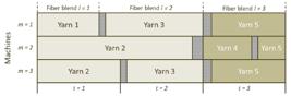
Illustrative production plan of a spinning industry. Adaptation from (^{Camargo et al., 2012}).

Very few studies have attempted to develop mathematical models for such a blending problem of cotton bales. ^{Greene et al. (1965}) proposed an initial model in which the objective is to minimize the raw material costs and in which decision variables were linear, that is, part of a cotton bale can be selected to make up the blend. Besides the classical quality constraints, ^{Zago (2005}) developed a formulation that considered the entire bale, and consequently, the decision variables were constrained by integer values. Ideas from Zago’s formulation are applied to our problem. The point of this paper is to select a set among a large number (Z ⁰) of stored bales (with different attributes) that meets the quality specifications. We are interested in controlling the G colors present in the cotton fibers. Therefore, maximum and minimum limits must define the necessary fiber characteristics for the blend. The reduction of the difference between the blends is an objective to be achieved. To maintain the availability of the colors present in the bales in inventory, we follow an approach proposed by ^{Zago (2005}) to minimize the percentage changes in the availability of the bales. Therefore, as the blends contain different number of bales, the relative difference must be calculated and managed. The same applies to the availability of the colors in the inventory.

This decision allows us to reproduce the previous blend with a minimum (or no) attribute variability. In contrast to the classic blending problem, the quantity of raw material used must be represented by integer decision variables. The cotton bales are not inserted in pieces of the production process.

The next model (22)-(32) relates to the blending problem and applies to the cotton bale selection that ensures the quality specifications. The additional indices, parameters and decision variables to be used in this part of the formulation are the following:

Indices g = 1,..., G color grade levels (fiber attribute). Parameters I g 0 initial bale inventory level of color grade attribute g; Z 0 total number of bales in the initial inventory; w weight of one cotton bale; q amount of cotton bales for a blend load: q=C/w; α ¯ g k maximum percentage of the color grade attribute g in the blend of type k; α g k minimum percentage of the color grade attribute g in the blend of type k; f gk amount of bales with color grade g used in the last blend load of type k; v ¯ g k maximum variation allowed for the color grade attribute g in the blend of type k (in percentage). Variables I g f final inventory level of bales with color grade g; Z f total number of bales in the final inventory; 𝒜g variation (in percentage) of bales with color grade g in the inventory; ℋgk variation of bales with color grade g between blends of type k; D k number of blend loads of type k needed for production; B k takes 1, if one or more blend loads of type k is used; 0 otherwise; F gk number of bales with color grade g used in the blend load of type k.

Indices
g = 1,..., G	color grade levels (fiber attribute).
Parameters
$I_g^0$	initial bale inventory level of color grade attribute g;
Z 0	total number of bales in the initial inventory;
w	weight of one cotton bale;
q	amount of cotton bales for a blend load: $q=⌈C/w⌉$;
${\overline{\alpha }}_{gk}$	maximum percentage of the color grade attribute g in the blend of type k;
${\underline{\alpha }}_{gk}$	minimum percentage of the color grade attribute g in the blend of type k;
f gk	amount of bales with color grade g used in the last blend load of type k;
${\overline{v}}_{gk}$	maximum variation allowed for the color grade attribute g in the blend of type k (in percentage).
Variables
$I_g^f$	final inventory level of bales with color grade g;
Z f	total number of bales in the final inventory;
𝒜g	variation (in percentage) of bales with color grade g in the inventory;
ℋgk	variation of bales with color grade g between blends of type k;
D k	number of blend loads of type k needed for production;
B k	takes 1, if one or more blend loads of type k is used; 0 otherwise;
F gk	number of bales with color grade g used in the blend load of type k.

$\mathbf{\text{Minimize}}\lambda \text{'}\sum _{g=1}^G{\mathcal{A}}_g+\lambda »,»\; \circledR ,\circledR \; \S ,\S \; ­,­\; ¹,¹\; ²,²\; ³,³\; ß,ß\; Þ,Þ\; þ,þ\; \times ,\times \; Ú,Ú\; ú,ú\; Û,Û\; û,û\; Ù,Ù\; ù,ù\; ¨,¨\; Ü,Ü\; ü,ü\; Ý,Ý\; ý,ý\; \yen ,\yen \; ÿ,ÿ\; \P ,\P \sum _{k=1}^K\sum _{g=1}^G{\mathcal{H}}_{gk}$ (22)

Subject to blending constraints:

$\left|\frac{I_g^0}{Z^0}-\frac{I_g^f}{Z^f}\right|={\mathcal{A}}_g\forall g$ (23)

$D_k\le L·B_k\forall k$ (24)

$\left({\underline{\alpha }}_{gk}-1+B_k\right)·q\le F_{gk}\le \left({\overline{\alpha }}_{gk}+1-B_k\right)·q\forall g,k$ (25)

$\left|F_{gk}-f_{gk}\right|\le \left({\mathcal{H}}_{gk}+1-B_k\right)·q\forall g,k$ (26)

${\mathcal{H}}_{gk}\le {\overline{v}}_{gk}\forall g,k$ (27)

$\sum _{g=1}^G{F}_{gk}=q·B_k\forall k$ (28)

$Z^f=Z^0-\sum _{k=1}^{K}q·D_k$ (29)

$I_g^f=I_g^0-\sum _{k=1}^K{D}_k·F_{gk}\forall g$ (30)

$B_k\in \left\{0,1\right\};F_{gk}\in {\mathrm{\mathbb{Z}}}_{+}\forall g,k$ (31)

$\text{all other variables are non-negative and continuous.}$ (32)

Objective function targets to minimize the variations of the attributes in the inventory (first summation) and aims to minimize the variations between blends (second summation). λ' and λ'' allow the decision maker to choose the priority, assigning different weights. Variable 𝒜 _g holds the inventory variation of bales with color grade g, while ℋ _gk holds the variation of bales with color grade g between blends of type k. In the following paragraph, we can see an example of how variability is calculated. Constraints (23) allocate the variation of the percentage of each attribute in the inventory using variables 𝒜 _g . Note that $I_g^0/Z^0$ represents the ratio of bales with color grade g to the inventory at the beginning of the planning horizon. $I_g^f/Z^f$ is the ratio of bales with color grade g to the inventory at the end of the planning horizon. As $I_g^f$ and Z ^f are decision variables, constraints (23) are nonlinear. Remark (1) shows an approach to deal with this nonlinearity. In constraints (24), if one or more blend loads of type k are used (i.e. $D_k>0$), B _k takes one. Constraints (25) denote the classical requirements to determine quality limits for attribute g of blend type k. Note that these constraints are active for k such that B _k = 1, that is, only for blend loads used in the planning. Constraints (26) account for the variation of the percentage of each attribute g between blends that belong to the same type k (yarn family). Constraints (27) limit the maximum percentage variation of each attribute g between blends to a value predefined by the decision-maker. The total number of bales in each blend load is accounted by (28), whereas the total number of bales consumed within the planning horizon is determined by (29). Similarly, equations (30) define the number of stored bales of each attribute at the end of the planning horizon. Constraints (31)-(32) enforce the binary, integrality and non-negative requirements for the variables.

To illustrate the objective function, consider the following example. Suppose that a blend k = 1 must be prepared with 150 bales. The initial inventory of bales is $I^0=\left(150,350,750,200,100\right)$ with a total $Z^0=1,550$ bales. In the previous blend k = 1 the following bales were used: $f_{g1}=\left(10,40,60,60,10\right)$. The variation between blends considers the F _gk values to be used after optimization. The variation in the bale inventory includes the remaining $I_g^f$ values after the use of bales. Thus, if $F_{g1}=\left(9,35,63,32,11\right),\left|F_{g1}-f_{g1}\right|=\left(1,5,3,2,1\right)$. Then $\sum _{g=1}^G{\mathcal{H}}_{g1}=0.08$, i.e., there is a 8% variation in the bales between previous and current blends. Similarly, $I_g^f=\left(141,315,687,168,89\right)$ with Z ^f = 1, 400 remaining bales in inventory, $\left|\frac{I_g^0}{Z^0}-\frac{I_g^f}{Z^f}\right|=\left(0.0039,0.0003,0.0068,0.0090,0.0009\right)$. Thus, $\sum _{g=1}^G{\mathcal{A}}_g=0.0209$, i.e., there is a variation of 2.09% in the characteristics of the fibers present in the inventory. By the problem definition, variabilities should be minimized.

3.3 The integrated formulation

This model incorporates features of the multi-stage hybrid lotsizing and scheduling constraints from ^{Camargo et al. (2012}), the simple plant location reformulation ^{Krarup & Bilde (1977}) and the blending constraints from ^{Zago (2005}). The problem solution draws up a production plan in which the blend loads are sequenced and their required qualities are determined. Moreover, having synchronized quality, the yarn amount (and its sequence) to be produced on each machine is established.

Constraints (33) aim to integrate the lotsizing and scheduling sub-problem - constraints (2)-(21) - with the blending sub-problem - constraints (23)-(32). They count the number of blend loads of each type k needed to meet the production plan.

Integrating constraints:

$D_k=\sum _{l=1}^L{U}_{lk}\forall k$ (33)

Also, three objective functions are identified during the decision-making process. Specific factors that could influence the production-blending decisions ought to be considered jointly. Therefore, the decision-maker can manipulate the weight of each decision. λ represents the influencing weighs of each production-blending decisions in the final objective function (34). However, in case the decision-maker considers λ ₁ = λ ₂ = λ ₃, the terms related to λ ₂ and λ ₃ are used only as a tiebreaker (due to their magnitudes) between the production plans with the lowest costs of inventory, backlogging and machine setup.

The integrated lotsizing, scheduling and blending decisions in the spinning model is defined below.

$$\begin{gathered} \mathbf{\text{Minimize}}{\lambda }_1·(\sum _{m=1}^M\sum _{i=1}^N\sum _{t=1}^T\sum _{l=1}^L\sum _{t\text{'}=1}^T{c}_{itt\text{'}}·X_{mitlt\text{'}}+\sum _{m=1}^M\sum _{i=1}^N\sum _{j=1}^N\sum _{t=1}^T\sum _{l=1}^L{\sigma }_{mij}·Y_{mijtl} \\ +\sum _{l=1}^L{r}_l·R_l)+{\lambda }_2·\left(\sum _{g=1}^G{\mathcal{A}}_g\right)+{\lambda }_3·\left(\sum _{k=1}^K\sum _{g=1}^G{\mathcal{H}}_{gk}\right) \end{gathered}$$ (34)

Subject to:

$$\begin{gathered} \left(2\right)-\left(21\right), \\ \left(23\right)-\left(33\right). \end{gathered}$$

The aforementioned model is nonlinear due to requirements (23) and (30). The following remark shows how such a feature can be tackled. Functions max, min and module can be linearized straightforwardly.

Remark 1.As Z^f,$I_g^f$, D_kand F_gkare decision variables, constraints (23) and (30) are nonlinear. In fact, constraints (29) and (30) are modeled only to define the variables Z^fand$I_g^f$used in constraint (23). Given equations (30) and the assumption$Z^f=Z^0-\sum _{k=1}^{K}q·D_k$, requirements (23) can be rewritten as

$\sum _{k=1}^K{D}_k·\left|F_{gk}-q·\frac{I_g^0}{Z^0}\right|={\overline{\mathcal{A}}}_g\forall g,$ (35)

Where ${\overline{\mathcal{A}}}_g$ denotes the deviation between the planned F _gk and the expected usage of attribute g (see details in Appendix 6).

Let ${\mathcal{Z}}_{k,l_k}$ be one, if D _{k = l} ; and 0 otherwise, where l _{k = 0} , . . . , L. That is, the integer number D _k is codified as a binary summation as follows:

$D_k=\sum _{l_k=0}^L{l}_k·{\mathcal{Z}}_{k,l_k}\forall k;$ (36)

$\sum _{l_k=0}^L{\mathcal{Z}}_{k,l_k}=1\forall k.$ (37)

Finally, let l₁, l₂, . . . , l_Kbe indices$\in \left\{0,\dots ,L\right\}$and ℳ be a big number, constraints (35) are defined as:

$$\begin{gathered} l_1·\left|F_{g1}-q·\frac{I_g^0}{Z^0}\right|+l_2·\left|F_{g2}-q·\frac{I_g^0}{Z^0}\right|+\dots +l_K·\left|F_{gK}-q·\frac{I_g^0}{Z^0}\right| \\ \le {\overline{\mathcal{A}}}_g+\mathcal{M}·\left(K-{\mathcal{Z}}_{1,l_1}-{\mathcal{Z}}_{2,l_2}-\dots -{\mathcal{Z}}_{K,l_K}\right)\forall g,l_1,l_2,\dots ,l_K. \\ \square \end{gathered}$$

$$\begin{gathered} \sum _{k=1}^K{l}_k·\left|F_{gk}-q·\frac{I_g^0}{Z^0}\right|\le {\overline{\mathcal{A}}}_g+\mathcal{M}·\left(K-\sum _{k=1}^K{\mathcal{Z}}_{k,l_k}\right)\forall g,l_1,l_2,\dots ,l_K. \\ \square \end{gathered}$$ (38)

The mathematical model in this paper considers the raw cotton non-used in the production as residue (R _l ). Some industrial processes do not allow this residue and it must be fully used to produce yarns. Moreover, without loss of generality, the model takes only into account the color grade as the essential attribute to define the yarn quality. Company policies may also consider other attributes as essential. Below, remarks 2 and 3 consider generalizations for the previous formulation: extensions to deal with raw cotton residue and to manage the quality of more than one fiber attribute.

Remark 2.

We assume in model (1)-(21) that the opening-and-blending machine capacity is completely used. It is represented in constraints (14) by adding a variable Rl to account for the unused cotton. The costs of this residue are properly added in the objective function.

Without loss of generality, the residue can also be used for make-to-stock ¹ production. This specificity can appear in practice. Thus we define $X_{mitl}^{MTS}$ as the make-to-stock production in machine m of yarn i in period t using the lth blend load. On the other hand, $X_{mitlt\text{'}}^{MTO}$ represents the make-to-order production as previously discussed. A couple of constraints should be incorporated to enforce these production cases:

$X_{mitl}=X_{mitl}^{MTS}+\sum _{t\text{'}=1}^T{X}_{mitlt\text{'}}^{MTO}\forall m,i,t,l;$ (39)

$\sum _{m=1}^M\sum _{i=1}^N\sum _{t=1}^T{X}_{mitl}^{MTS}=R_1\forall l.$ (40)

The total production is used in constraints (39) for make-to-stock and for make-to-order decisions. Constraints (40) link the raw material residue to the make-to-stock production. For this assumption, some constraints must be changed. Constraints (5), (6) and (9) are respectively replaced by

$\sum _{m=1}^M\sum _{i=1}^N\sum _{l=1}^L{X}_{mitlt\text{'}}^{MTO}=d_{it\text{'}}\forall i,t\text{'};$ (41)

${\mu }_{mitl}^f-{\mu }_{mitl}^s\ge \sum _{j=1}^N\left(s_{mji}·Y_{mjitl}\right)+p_{mi}·X_{mitl}\forall m,i,t,l;$ (42)

$p_{mi}·X_{mitl}\le \sum _{j=1}^N{Y}_{mjitl}+{\alpha }_{mitl}\forall m,i,t,l.$ (43)

Constraints (41) ensure that the yarn demand will be fulfilled. Requirements (42) and (43) accommodate the new production variables X_mitl. Naturally, the objective function has to be updated. □

Remark 3.When more than one fiber attribute must be managed, some constraints and variables have to be changed in the model, for instance, the company policy required to control the color grade (g = 1, . . . , G) and fiber length (b = 1, . . . , B) attributes. The inventory level variable is reformulated to incorporate the fiber length attribute$\left(I_{gb}^f\right)$and to inform the number of bales with color grade g and fiber length b in the inventory at the end of the planning horizon. Similar reformulations are done in variables F_gbkand parameters$I_{gb}^0$and f_gbk. Moreover, variables 𝒜_gand ℋ_gkare specific for the color grade attribute and must be replicated for the fiber length, as well as the parameters${\overline{v}}_{gk},{\overline{\alpha }}_{gk}$and${\underline{\alpha }}_{gk}$. Regarding these assumptions, it is straightforward to accommodate constraints related to additional attributes in the model. □

3.4 Illustrative example

The usage of the integrated model is illustrated by a small example provided in Tables 1, 2 and 3. The raw material inventory consists of 730 cotton bales. Two types of fiber blends are managed in the example. The inventory and quality limits for the attribute color grade is defined in Table 3, as well as the latest blend loads. The maximum variation allowed by the company policies for the color grade between blends is 7%.

Table 1
Data parameters.

Product	Family k	d it			p mi	c itt'
		t = 1	t = 2	t = 3		t < t'	t > t'
i = 1	1	4,666	0	0	0.000150	0.0017	0.17
i = 2	1	20,000	10,247	0	0.000097	0.0017	0.17
i = 3	1	0	4,067	0	0.000540	0.0017	0.17
i = 4	2	0	0	3,243	0.000185	0.0017	0.17
i = 5	2	0	0	15,815	0.000141	0.0017	0.17

Table 2
Setup times and setup costs (s _mji /σ _mji ).

Product	1	2	3	4	5
1	0.0/0.0	0.031/3.1	0.039/3.9	0.066/6.6	0.060/6.0
2	0.047/4.7	0.0/0.0	0.042/4.2	0.066/6.6	0.050/5.0
3	0.045/4.5	0.040/4.0	0.0/0.0	0.060/3.0	0.070/5.0
4	0.063/6.3	0.063/6.3	0.063/6.3	0.0/0.0	0.030/3.0
5	0.065/6.5	0.062/6.2	0.060/6.0	0.050/5.0	0.0/0.0

Table 3
Data parameters of the raw material inventory for the illustrative example.

		Color grade
		White	Light spotted	Spotted	Tinged
Initial inventory ($I_g^0$)		230	250	200	50
Number of bales used in latest load ( f gk )	k = 1	91	8	1	0
	k = 2	62	18	18	2
Minimum limit (${\underline{\alpha }}_{gk}$)	k = 1	0.85	0	0	0
	k = 2	0.6	0	0	0
Maximum limit (${\overline{\alpha }}_{gk}$)	k = 1	1	0.16	0	0
	k = 2	1	0.25	0.2	0.02

The number of machines is M = 3 and the common resource capacity is C = 20, 000 kilos. Machine 1 is set up for product i = 1 at the beginning of the planning horizon and machines 2 and 3 are set up for product i = 2. The planning horizon entails T = 3 time periods. Products 1, 2 and 3 require the same attributes and belong to product family k = 1, whilst products 4 and 5 are part of product family k = 2. Inventory $\left(c_{itt\text{'}}|t<t\text{'}\right)$ and backlogging costs $\left(c_{itt\text{'}}|t>t\text{'}\right)$ are equal for all periods. Production rates (p _mi ), setup costs and times (s _mji and σ _mji ) do not vary between machines.

An optimal lotsizing and scheduling plan is illustrated in Table 4. The most relevant non-zero solution values for the instance are given. It should be noted that ${\mu }_{mitl}^s$ and ${\mu }_{mitl}^f$ represent the starting and finishing times to produce product i on machine m in period t using the lth common resource batch; Y _mijtl takes on 1, if there is a changeover on machine m from product i to product j in period t, using the lth common resource batch; α _mitl equals 1, if the machine m is set up for product i in the period t using the lth common resource batch; X _mitlt1' denote the production variables. As can be seen, a production plan is determined. The required blend loads are U ₁₁ = 1, U ₂₁ = 1 and U ₃₂ = 1, that is, $D_k=\left\{2,1\right\}$ and the production sequences for the spinning machines are 1-3-5, 2-3-4-5 and 2-5.

Table 4
Optimal production plan from the integrated lot sizing, scheduling and blending.

	t = 1	t = 2	t = 3
m = 1	α1111 = 1	α1322 = 1	α1333 = 1
	${\mu }_{1111}^s:{\mu }_{1111}^f=0:0.7$	${\mu }_{1322}^s:{\mu }_{1322}^f=1:2$	Y13533 = 1
	X11111= 4667	X13222= 1851.9	${\mu }_{1533}^s:{\mu }_{1533}^f=2:3$
	Y11312 = 1		X15333= 6595.7
	${\mu }_{1313}^s:{\mu }_{1312}^f=0.7:1$
	X13122= 474.4
m = 2	α2211 = 1	α2322 = 1	α2433 = 1
	${\mu }_{2211}^s:{\mu }_{2211}^f=0:0.7$	${\mu }_{2322}^s:{\mu }_{2322}^f=1:1.94$	${\mu }_{2433}^s:{\mu }_{2433}^f=2:2.6$
	X22111= 7266.2	X23222= 1740	X24333= 3243
	${\mu }_{2212}^s:{\mu }_{2212}^f=0.7:1$	Y23422 = 1	Y24533 = 1
	X22121= 2424.5	${\mu }_{2422}^s:{\mu }_{2422}^f=1.94:2$	${\mu }_{2533}^s:{\mu }_{2533}^f=2.6:3$
	Y23312 = 1		X25333= 2624.4
m = 3	α3211 = 1	α3222 = 1	α3233 = 1
	${\mu }_{3211}^s:{\mu }_{3211}^f=0:0.7$	${\mu }_{3222}^s:{\mu }_{3222}^f=1:2$	Y32533 = 1
	X32111= 7266.2	X32222= 10247	${\mu }_{3533}^s:{\mu }_{3533}^f=2:3$
	${\mu }_{3212}^s:{\mu }_{3212}^f=0.7:1$		X35333= 6737.6
	X32121= 3043.1
Stock level	X13122= 474.41
Residue level	R1 = 801.63	R2 = 218.37	R3 = 942
Value of solution: 33.33

Table 5 illustrates the final inventory of cotton bales and the number of bales of each attribute determined for each blend type. The variation of each color grade is given in percentage.

Table 5
Optimal blending solution to the integrated approach.

		Color grade
		White	Light spotted	Spotted	Tinged
Final inventory ($I_g^f$)		0	200	180	50
Used bales (F gk )	k = 1	85	15	0	0
	k = 2	60	20	20	0
Variation between blends (ℋgk )	k = 1	0	0	0.1	0
	k = 2	0.2	0.7	0.2	0.2

4 INTEGRATED VS. HIERARCHICAL ANALYSIS

In order to show that the lotsizing and scheduling decisions should not be taken without considering the blending decision jointly, the integrated lotsizing, scheduling and blending model is compared to the hierarchical approach. The integrated model can be decoupled into a lotsizing and scheduling sub-model and a blending sub-model by ignoring constraints (33): $D_k=\sum _{l=1}^L{U}_{lk},\forall k$.Figure 4 illustrates the steps for a hierarchical solution to the problem.

Figure 4
Step flow for hierarchical production-scheduling and blending.

First, this hierarchical approach determines the lot sizing and scheduling. From the sequence of the blends, one can implicitly obtain the number of blends of each type needed to carry out the production, that is, Dk is the input data for the blending definition. Thus the blending solution gives the set of bales that satisfy the quality specifications for the yarns. The lotsizing and scheduling formulation reads as follows:

Lot sizing and scheduling:

Minimize

$$\begin{gathered} {\lambda }_1·(\sum _{m=1}^M\sum _{i=1}^N\sum _{t=1}^T\sum _{l=1}^L\sum _{t\text{'}=1}^T{c}_{itt\text{'}}·X_{mitlt\text{'}}+\sum _{m=1}^M\sum _{i=1}^N\sum _{j=1}^N\sum _{t=1}^T\sum _{l=1}^L{\sigma }_{mij}·Y_{mijtl} \\ +\sum _{l=1}^L{r}_l·R_l) \end{gathered}$$

Subject to:

$$\begin{gathered} \left(2\right)-\left(19\right) \\ {Y}_{mijtl}\in \left\{0,1\right\};U_{lk}\in \left\{0,1\right\};P_{tl}^s\in \left\{0,1\right\};P_{tl}^f\in \left\{0,1\right\}\forall m,i,j,t,l,k \\ \text{all other variables are non-negative and continuous.} \end{gathered}$$

The blending problem is formulated as follows:

Blending:

$\mathbf{\text{Minimize}}\left(\sum _{g=1}^G{\mathcal{A}}_{\mathbf{g}}\right)+{\lambda }_3·\left(\sum _{k=1}^K\sum _{g=1}^G{\mathcal{H}}_{gk}\right)$

Subject to:

$$\begin{gathered} \left(23\right)-\left(30\right) \\ {B}_k\in \left\{0,1\right\};F_{gk}\in {\mathrm{\mathbb{Z}}}_{+}\forall g,k \\ \text{all other variables are non-negative and continuous.} \end{gathered}$$

4.1 Sensitivity analysis

The integrated and hierarchical approaches can be compared by applying both to a specific set of data based on a real-world problem, in which the raw material inventory consists of 3,847 cotton bales. Company policy considers four attributes as crucial in terms of defining the blend: supplier, color, leaf grade, and short fiber index (SFI), respectively, with 18, 3, 2 and 2 different possible values. All costs are derived from the opportunity cost per yarn package unit. Other parameters related to the production environment (e.g., setup and processing times and machine capacities) are derived or similar to the real data. The number of yarns N is five and they belong to two product families K.

Moreover, K is the number of different types of blends. The number of spinning machines M is three. The number of periods T is equal to five, and the maximum number of blend load in the planning horizon L is fixed at six. The opening-blending machine has the capacity set to 100 bales of 200 kilograms each. Demands for yarns are obtained from an order book of the spinning mill. The complete instance is available on GitHub.

The models were generated in OPL language and solved by the CPLEX mixed-integer solver version 12.10. Tests were conducted on an Intel computer at 2.7 GHz with 16 GB of RAM. The running time was limited to 10 minutes for each test. In all tests, the optimal solution was found within the time limit.

Figure 5 depicts the behavior of the integrated and hierarchical approaches to find feasible plans under an upper bound to the variability between blends (VBB). VBB means ${\overline{v}}_{gk}$ in the mathematical formulation. Figure 6 shows the variability of the attributes in the inventory, considering the limitation to VBB given by the production plans of both integrated and hierarchical approaches. Several values to VBB were checked. A comparison of the integrated and hierarchical approaches relies on the unfulfilled demand and the variation of the attributes in the inventory. Figures 5 and 6 must be analyzed together. As can be seen in Figure 5, regardless of the VBB limit, unfulfilled demand given by the hierarchical approach is constant. The production plan is defined at the first step (lotsizing and scheduling problem) and does not consider any information about the blending requirements; that is, the blend sequence is given in the production plan without information if it is possible to ensure its quality. For VBB limits greater than 0.07, the results of the integrated model resemble those from the hierarchical approach. On the other hand, the integrated approach finds solutions with higher production costs for VBB limited to 0.07 or less. By looking at the variation of the attributes in the inventory (Figure 6), the hierarchical approach is not able to find solutions at the blending step when the VBB is limited to 0.07 or less.

Figure 5
Integrated versus hierarchical approach - production cost behavior.

Figure 6
Integrated versus hierarchical approach - attribute variability in the inventory.

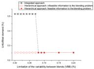
When company policies require yarn production with hard quality constraints, the hierarchical approach corresponds to a trial and error approach. When $D_k^{\text{'}}$ provides an unfeasible solution, a new lotsizing and scheduling solution is requested with an additional constraint to avoid $D_k^{\text{'}}$. In practice, the hierarchical approach may require several iterations between the problems to deliver a production plan with blending constraints satisfied. In some cases, feasible solutions could not be found. However, the integrated approach delivers the optimal D _k concerning the strict quality constraints. Blending requirements are met waiving the best production decision. This fact can be seen in Figure 5, where high unfulfilled demand represents the backorder.

As one can see in Figure 6, the hierarchical approach delivers blends without variation of the attributes in the inventory if Dk is feasible. The integrated approach should also deliver blends without variation. However, the values reported by the integrated approach can be explained by blending decisions having low weight (λ ₂ and λ ₃) in the objective function. Decisions of a lower weight are used as tiebreakers for solutions with similar decisions of a higher weight (λ ₁). However, lower weight decisions have little influence on the absolute value of the objective function (and, consequently, on the optimality gap).

It is worth noting in Figure 6 that the hierarchical approach delivers blends without variation of the attributes in the inventory. It happens because the cotton inventory has enough quality to ensure minimal variation between blends VBB less than 0.07 without variation of the attributes in the inventory. Then in case VBB is limited to 0.08, solutions are dominated. It is possible to easily obtain the minimum VBB admitted by inventory to fulfill the yarn demand. It is also clear that variations of attributes in the inventory increase when limitation on variability between blends (VBB) decreases.

Consequently, the best of both worlds - the combined integrated and hierarchical approaches - can better achieve the objectives defined for integrated lot sizing, scheduling and blending.

5 PARTIAL INTEGRATED APPROACH FOR PRODUCTION SCHEDULING AND BLENDING DECISIONS

The partial integrated approach for coordinating production and blending planning attempts to combine features from those above integrated and hierarchical approaches. The aim is to provide the lotsizing and scheduling problem with blending constraints to foster production plans having strict quality requirements. On the other hand, specific decisions for minimizing attribute variation can be found by the blending model without the optimality gap hurdle of the integrated approach. The partial integrated approach for production scheduling and blending is written as follows:

$\mathbf{\text{Minimize}}\sum _{m=1}^M\sum _{i=1}^N\sum _{t=1}^T\sum _{l=1}^L\sum _{t\text{'}=1}^T{c}_{itt\text{'}}·X_{mitlt\text{'}}+\sum _{m=1}^M\sum _{i=1}^N\sum _{j=1}^N\sum _{t=1}^T\sum _{l=1}^L{\sigma }_{mij}·Y_{mijtl}+\sum _{l=1}^L{r}_l·R_l$ (44)

Subject to

$$\begin{gathered} \mathbf{\text{Lotsizing and scheduling constrainst:}}\left(2\right)-\left(19\right) \\ \mathbf{\text{Some blending constraints:}}\left(24\right)-\left(28\right) \\ {B}_k\in \left\{0,1\right\};F_{gk}\in {\mathrm{\mathbb{Z}}}_{+}\forall g,k \\ {Y}_{mijtl}\in \left\{0,1\right\};U_{lk}\in \left\{0,1\right\};P_{tl}^s\in \left\{0,1\right\};P_{tl}^f\in \left\{0,1\right\}\forall m,i,j,t,l,k \\ \text{all other variables are non-negative and continuous.} \end{gathered}$$

As can be observed, the partial integrated production and blending planning takes into account some of the blending requirements. Minimal variations between blends are ensured, but those related to attribute variation in the inventory are skipped. In the same way as in the hierarchical approach, the blending sequence $\left(\sum _{l=1}^L{U}_{lk}=D_k\right)$ defines the input data for the blending model. However, unlike the hierarchical case, the partial integrated approach provides feasible parameters D _k . Thus the blending solution can give the set of bales that fulfills the quality specifications as the feasibility is tested in advance. Note that the blending model is the same as that of the hierarchical approach (see Section 4).

Remark 4.In the partial integrated approach, some blending constraints (24)-(28) are applied to both lotsizing and scheduling problem and blending problem. This strategy enforces the lotsizing and scheduling formulation to deliver a feasible plan of blend loads. On the other hand, those constraints can not be omitted in the blending model else, the variability between blends is not taken into account in the bale selection. □

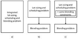
Figure 7 compares the different proposed approaches. The integrated approach (7a) solves the problem in a single process while the hierarchical approach (7b) firstly deals with the lotsizing and scheduling problem and determines the blending decisions afterward. The partial integrated approach (7c) solves the lotsizing and scheduling problem considering some blending constraints to find a feasible production plan to the blending problem subsequently solved.

Figure 7
Comparison of the proposed approaches to find a solution.

The partial integrated approach is also analyzed in Figure 8, which depicts both the unfulfilled demand and the variation of the attributes in the inventory. Note that the green squares refer to unfulfilled demand and the blue triangles to the total variability of the attributes in the inventory.

Figure 8
The partial integrated approach - attribute variability in the inventory and production cost behavior.

From these results, the partial integrated approach can determine feasible production plans having strict quality specifications and can define the best set of cotton bales. As can be seen, the unfulfilled demand resembles that delivered by the integrated approach and the attribute variation caused in the inventory is optimal, which is similar to the single blending problem (compare Figure 8 against Figures 5 and 6).

6 CONCLUSION

In this paper, we have discussed the importance of integrating the production and blending planning problems dealing with attribute variability constraints. Besides the traditional lotsizing and scheduling decisions, the planning should determine which cotton bales must be part of the blend (the raw material). The problem is to determine the production level and sequence for the yarns and the cotton blends. It provides information on the number of blends and cotton bales needed for production in the planning horizon. Having this information, the blending problem must define which stored bales should be used to ensure yarn quality and to keep a raw material inventory able to reproduce the blends with a minimum attribute variation. A mathematical model for integrated lotsizing, scheduling and blending problem is proposed. The basic idea behind this approach is to simultaneously optimize decision variables of different functions that have traditionally been optimized sequentially. The hierarchical approach is proposed so that the lotsizing and scheduling problem is solved a priori. Then, the blending problem defines the set of cotton bales that meets the quality requirements.

The integrated model and the hierarchical approach are compared, and from the results, we note the influence of the raw material inventory on lotsizing and scheduling decisions. The analysis of the results indicates that a feasible production plan can only be obtained if blending related constraints are taken into account. When the product quality has to be controlled, it is reasonable to suggest the integration of lotsizing, scheduling and blending decisions. Moreover, the partial integrated approach is a purpose that incorporates some blending constraints to ensure the yarn quality when planning the production in the first phase. In addition, the partial approach has the accuracy of the blending phase to find the set of cotton bales with minimal variations in the inventory and between blends.

In conclusion, production planning without taking into account raw material requirements can often be a source of production problems. It can generate impractical plans or cause customer dissatisfaction and a decrease in the price of the product in case of not complying with yarn specifications. We believe our study has shown that, considering the restricted quality conditions, coordinating production and blending can be extremely important.

Further research towards multi-objective decisions can assist the decision-maker to define a production plan and choose cotton blends with the best trade-off between the attribute variability and production costs. A set of experiments should indicate the strengths and advantages of each of the mathematical models, in terms of the quality of the solutions provided and the computational burden to solve them. Moreover, the analysis of the integrated problem might help the purchasing department on how to define the orders for cotton bales and the sales department on which yarn type can be produced and sold. The purchase can also be oriented by the production plan to keep the attribute variability in the inventory and to indirectly maximize the reproduction of blends. Other industries (such as coffee, emulsified meat, pulp and paper, etc.) may benefit from the production planning approaches developed in this paper. In this direction, the development of an advanced planning and scheduling system (APS) that covers the production planning functionality for these types of industries can follow the framework proposed in ^{Fachini et al. (2018}).

References

• ¹
  ADMUTHE LS & APTE SD. 2009. Optimization of spinning process using hybrid approach involving ANN, GA and linear programming. Proceedings of the 2nd Bangalore Annual Compute Conference, pp. 1-4.
• ²
  CAMARGO VCB, TOLEDO FMB & ALMADA-LOBO B. 2012. Three time-based scale formulations for the two-stage lot sizing and scheduling in process industries. Journal of the Operational Research Society, 63: 1613-1630.
• ³
  CAMARGO VCB, TOLEDO FMB & ALMADA-LOBO B. 2014. HOPS - Hamming-Oriented Partition Search for production planning in the spinning industry. European Journal of Operational Research, 234(1): 266-277.
• ⁴
  CLAASSEN G, GERDESSEN JC, HENDRIX EM & VAN DER VORST JG. 2016. On production planning and scheduling in food processing industry: Modelling non-triangular setups andproduct decay. Computers & Operations Research, 76: 147-154.
• ⁵
  COPIL K, WÖRBELAUER M, MEYR H & TEMPELMEIER H. 2017. Simultaneous lotsizing and scheduling problems: a classification and review of models. OR spectrum, 39(1): 1-64.
• ⁶
  CRAMA Y, POCHET Y & WERA Y. 2001. A discussion of production planning approaches in the process industry. CORE Discussion Papers 2001042. Université catholique de Louvain, Center for Operations Research and Econometrics (CORE).
• ⁷
  CUNHA AL, SANTOS MO, MORABITO R & BARBOSA-PÓVOA A. 2018. An integrated approach for production lot sizing and raw material purchasing. European Journal of Operational Research , 269: 923-938.
• ⁸
  DREXL A & KIMMS A. 1997. Lot sizing and scheduling - Survey and extensions. European Journal of Operational Research , 99: 221-235.
• ⁹
  EL MOGAHZY Y. 2004. An Integrated Approach to Analyzing the Nature of Multi-component Fiber Blending - Part I: Analytical Aspects. Textile Research Journal, 78: 701-712.
• ¹⁰
  EL MOGAHZY Y. 2005. Specific approaches for cutting manufacturing cost and increasing profitability using the EFS system. In: EFS System Conference Presentations
• ¹¹
  EL MOGAHZY Y, FARAG R, ABDELHADY F & MOHAMED A. 2004. An Integrated Approach to Analyzing the Nature of Multicomponent Fiber Blending - Part II: Experimental Analysis of Structural and Attributive Blending. Textile Research Journal , 74: 767-775.
• ¹²
  FACHINI RF, ESPOSTO KF & CAMARGO VCB. 2018. A framework for development of advanced planning and scheduling (APS) systems in glass container industry. Journal of Manufacturing Technology Management, 29: 570-587.
• ¹³
  GREENE JH, CHATTO K, HICKS CR, COX CB, BAYNHAM TE & BAYNAM TEJ. 1965. Linear programming - Cotton blending and production allocation. Tech. rep.. International Business Machines Corporation (IBM); The Journal of Industrial Engineering.
• ¹⁴
  HAX AC & MEAL HC. 1973. Hierarchical integration of production planning and scheduling. Working papers 656-673. Massachusetts Institute of Technology (MIT), Sloan School of Management.
• ¹⁵
  KALLRATH J. 2002. Planning and scheduling in the process industry. OR Spectrum, 24: 219-250.
• ¹⁶
  KOPANOS GM, PUIGJANER L & GEORGIADIS MC. 2010. Optimal production scheduling and lot-sizing in dairy plants: the yogurt production line. Industrial & Engineering Chemistry Research, 49: 701-718.
• ¹⁷
  KRARUP J & BILDE O. 1977. Optimierung bei Graphenthe-oretischen und Ganzzahligen Probleme chap. Plant location, set covering and economic lot sizes: an O(mn) algorithm for structured problems, pp. 155-180. Basel: Birkhauser Verlag.
• ¹⁸
  PEREIRA DF, OLIVEIRA JF & CARRAVILLA MA. 2020. Tactical sales and operations planning: A holistic framework and a literature review of decision-making models. International Journal of Production Economics, 228: 107695.
• ¹⁹
  SOMAN CA, VAN DONK DP & GAALMAN G. 2004. Combined make-to-order and make-to-stock in a food production system. International Journal of Production Economics , 90: 223-235.
• ²⁰
  TOSCANO A, FERREIRA D & MORABITO R. 2019. A decomposition heuristic to solve the two-stage lot sizing and scheduling problem with temporal cleaning. Flexible Services and Manufacturing Journal, 31(1): 142-173.
• ²¹
  WÖRBELAUER M, MEYR H & ALMADA-LOBO B. 2019. Simultaneous lotsizing and scheduling considering secondary resources: a general model, literature review and classification. Or Spectrum, 41(1): 1-43.
• ²²
  ZAGO G. 2005. Otimização da composição da matéria prima para uma indústria têxtil de grande porte. Tech. rep.. Escola Politécnica, Universidade de São Paulo. São Paulo.
• ²³
  ZHU X & WILHELM WE. 2006. Scheduling and lot sizing with sequence-dependent setup: A literature review. IIE Transactions, 38: 987-1007.

• 1
  To read more about the combination of make-to-stock and make-to-order production in process industries, see (^{Soman et al., 2004}).

APPENDIX - A NEW PERCENTAGE VARIATION MEASURE

This appendix shows the steps to linearize constraints (23). Let $I_g^f=I_g^0-\sum _{k=1}^K{D}_k·F_{gk}$ be the final inventory level of bales with color grade g and $Z^f=Z^0-\sum _{k=1}^{K}q·D_k$ denotes the total number of bales in the final inventory; $I_g^0/Z^0$ represents the ratio of bales with color grade g to the inventory in the planning horizon beginning. Similarly, $I_g^f/Z^f$ refers to the ratio of bales with color grade g to the inventory in the planning horizon end. The percentage variation of bales with color grade g in the inventory is $\left(I_g^0/Z^0\right)-\left(I_g^f/Z^f\right)$.

Let $\left(I_g^0/Z^0\right)-\left(I_g^f/Z^f\right)$ be multiplied by a positive number for all g, the magnitude of the g g variations remain for the whole set.

For all g, we get:

$$\begin{gathered} \left(\frac{I_g^0}{Z^0}-\frac{I_g^f}{Z^f}\right)·Z^f=\frac{I_g^0}{Z^0}·Z^f-\frac{I_g^f}{Z^f}·Z^f \\ =\frac{I_g^0·Z^f}{Z^0}-I_g^f \\ =\frac{I_g^0·\left(Z^0-{\displaystyle \sum _{k=1}^K}q·D_k\right)}{Z^0}-\left(I_g^0-\sum _{k=1}^K{D}_k·F_{gk}\right) \\ =\frac{I_g^0·Z^0-I_g^0·{\displaystyle \sum _{k=1}^K}q·D_k}{Z^0}-I_g^0+\sum _{k=1}^K{D}_k·F_{gk} \\ =I_g^0-\frac{I_g^0·{\displaystyle \sum _{k=1}^K}q·D_k}{Z^0}-I_g^0+\sum _{k=1}^K{D}_k·F_{gk} \\ =\sum _{k=1}^K{D}_k·F_{gk}-\frac{I_g^0·{\displaystyle \sum _{k=1}^K}q·D_k}{Z^0}. \end{gathered}$$

Now, let ${\overline{\mathcal{A}}}_g$ be the percentage variation (with a new magnitude) of bales with color grade g in the inventory that should be minimized.

$$\begin{gathered} {\overline{\mathcal{A}}}_g=\left|\sum _{k=1}^K{D}_k·F_{gk}-\frac{I_g^0·\sum _{k=1}^K{D}_k·q}{Z^0}\right| \\ =\sum _{k=1}^K{D}_k·\left|F_{gk}-\frac{I_g^0·q}{Z^0}\right|. \end{gathered}$$

Clearly, assuming that magnitude of Z ^f , constraints (29) are dropped and constraints (23) are linearized. □

Publication Dates

• Publication in this collection
  11 June 2021
• Date of issue
  2021

History

• Received
  29 Jan 2020
• Accepted
  10 Mar 2021