General recursive solution for one-dimensional quantum potentials: a simple tool for applied physics

Solução recursiva geral para potenciais quânticos unidimensionais: uma ferramenta simples para física aplicada

ARTIGOS GERAIS

General recursive solution for one-dimensional quantum potentials: a simple tool for applied physics

Solução recursiva geral para potenciais quânticos unidimensionais: uma ferramenta simples para física aplicada

Sérgio L. Morelhão¹; André V. Perrotta

Instituto de Física, Universidade de São Paulo, São Paulo, SP, Brazil

ABSTRACT

A revision of the recursive method proposed by S.A. Shakir [Am. J. Phys. 52, 845 (1984)] to solve bound eigenvalues of the Schrödinger equation is presented. Equations are further simplified and generalized for computing wave functions of any given one-dimensional potential, providing accurate solutions not only for bound states but also for scattering and resonant states, as demonstrated here for a few examples.

Keywords: one-dimensional quantum potentials, numerical solutions, computational methods, Schrödinger equation.

RESUMO

Uma revisão do método recursivo proposto por S.A. Shakir [Am. J. Phys. 52, 845 (1984)] para solucionar autovalores de estados ligados da equação de Schrödinger é apresentado. As equações são ainda mais simplificadas e generalizadas para computar funções de onda em qualquer potencial unidimensional, fornecendo soluções acuradas não somente para estados ligados mas também para problemas de espalhamento e ressonância, como demonstrado aqui em alguns exemplos.

Palavras-chave: potenciais quânticos unidimensionais, soluções numéricas, métodos computacionais, equação de Schrödinger.

1. Introduction

Predicting physical properties of quantum systems has basically been treated as an eigenvalue problem. Since from single atoms and molecules up to nanostructured devices, chemical and electronic properties are determined by finding the eigenstates of the system's Hamiltonian. Methods of solving eigenvalue/eigenfunction problems are therefore an inevitable part of the quantum mechanic theory. In real systems, even one-dimensional problems can be quite difficult to solve analytically and often approximative, such as in perturbation theory, and/or numerical methods are required [1-6]. Semiconductor heterostructures are good examples of one-dimensional systems of technological interest where numerical solutions of the Schrödinger equation (SE) are often employed for self-consistent studies of electronic devices [7-11]. Studies of vibrational bound states of molecules in physical chemistry, as well as of other oscillatory systems in atomic and nuclear physics are treated as one-dimensional problems when summarized in the radial SE; they consist another class of important examples in which numerical methods are also often employed [12-15].

Although many procedures and algorithms are available in nowadays for solving the SE numerically - see for instance Refs. [16, 17], and references therein -, they are suitable to address specific problems on distinct fields of applied and theoretical physics. There is still a need for a general treatment that can be summarized into a single routine capable to solve equally well problems of confined modes by arbitrary potential as well as scattering problems in open systems. Moreover, all available numerical methods are essentially mathematical solutions of a differential equation, and hence the level of expertise required for dealing with these methods has kept them out of most physics and chemistry classrooms, even on graduate courses, where the demonstrative examples are still limited to a few cases of quantum potentials for which the analytical solutions are known.

More than 20 years ago, S.A. Shakir [18] presented a recursive method to find bound eigenvalues of the SE. It was a relatively simple method, closely related to those used in the field of optics for calculating the Fresnel amplitudes. In despite of its simplicity, and even of the fact of have been rediscovered a few years latter [19-21], this method has passed unnoted from the applied research fields until very recently [22].

In this work, instead of concerning with mathematical methods to solve the SE for bound and scattering states, we are concerned with alternative methods capable of providing better physical insight about the quantum world. In other words, methods that provide solutions of the SE without having to solve it mathematically. One class of alternative methods, which we call physical methods, is possible in one dimension. They are based on the elemental action of a given stationary force field on the wave function of the particle. Action that occurs at every step of a discretized potential energy function and it is qualitatively always the same, reflecting and transmitting the incident wave as in the Shakir's method [18]. However, here, the original formalism is simplified and generalized into a procedure for computing wave functions of any given potential whatever related to scattering, resonance, tunneling, or bound states, as demonstrated for a few examples. Physical method at their actual stage of development might require higher computational cost than mathematical methods, but offers versatility and exactness in return, as well as the fact that they can be explained and used even by undergraduate students and no-experts in numerical methods.

2. Theory

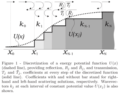
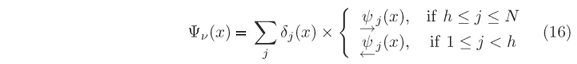
For a given potential energy function U(x), it is always possible to define the interval X = [x₀, x_N] such that outside its boundaries, i.e. for x Ï X, either the potential is constant or the amplitude of the wave function vanishes before appreciable variation of the potential. In this interval, the potential has been discretized into N steps, and we seek for stationary states with wave functions in the form

in which

and d_j(x) = 1 for x Î [x_j,x_j+1] and 0 otherwise. The under arrow indicates that this format will be used here for left-hand solutions, as better explained below.

Incremental distances dx_j = x_j+1-x_j, are small enough to guarantee a good numerical solution when taking U(x) = U(x_j)d_j(x), as shown in Fig. 1, so that

where j = . E and m stand for energy and mass of the particle, respectively.

To calculate the A_j and B_j amplitudes recursively, initial values at the boundaries of the interval X have to be provided. For instance, normalized solutions for incidence from the left-hand side, i.e. incidence from x < x₀, must have B_N = 0 and A₀ = 1. Conservation of the probability current imposes that

at every step of the potential, i.e. at every x_j. The prime symbol indicates the first derivative in x. Left-hand solutions are obtained by applying these conditions, Eqs. (4), first at x_N where B_N = 0 and

and then at x_N-1 where

and

and then at x_N-2 where

and A_N-2 is analogous to Eq. (7) when replacing N by N-1.

This is a recursive procedure, repeatable since j = N down to j = 1 as summarized by

where

and

All amplitudes are proportional to A₀, and within the condition assumed when defining the interval X, R_N+1 = 0.

Solutions for incident particles from the right-hand side, i.e. incidence from x > x_N, are obtained in analogous procedure, but for the sake of simplification in the final format of the recursive equations it is convenient to redefine the amplitudes as follow

and hence the wave function Y(x) of the stationary states will be calculated by using

instead of j(x).

By applying the continuity of

_j and '_j, as in Eqs. (4), analogous deduction of that in Eqs. (5)-(8) can be carried out but now starting from x₁ where C₁ = 0 up to x_N+1 where D_N+1 = 1 (for normalized solutions). It leads to the recursive equations

of the right-hand solutions where

and

for j = 1,2,..., N and ₀ = 0.

At certain energies E = _n, quantum confinements can occur at local minima of the potential in which U(x) < _n; given that each minimum is bounded on both sides by non-tunnelable barriers. Around one of such local minima, stationary wave solutions only exist when the waves reflected at both bounding ''walls'' interfere constructively to each other at any instant of time. It means that left-hand and right-hand scattering solutions must coexist in the confinement region, i.e. _j(x) = _j(x), which takes us back to Eqs. (11). Since B_j = A_jR_j+1 and C_j+1 = D_j+1

_j, as given by Eqs. (9) and (13), all amplitudes cancel each other out in Eq. (11) so that _jR_j+1 = exp(2ik_jdx_j). This latter relationship provides a criterion for numerical determination of the allowed modes in any confinement region of the potential since a minimization function such as

can be defined with j running over all values where U(x_j) < E. Then, the condition f(E) = 0 is fulfilled only for a set of discrete _n values of energy, corresponding to the eigenvalues of the one-dimensional SE at a given local minimum of U(x).

Eigenfunctions Y_n, of the energy eigenvalues _n, are computed as either _j(x) or _j(x) solutions in the classical allowed region around the minimum. But both solutions are required to compute the evanescent parts of the eigenfunctions inside the bounding walls and then it is necessary to match the amplitudes of these solutions at some point. If the hth step, for which U(x_h) < _n, is taken as the matching point, _h = _h and hence D_h = A_h(1+R_h+1)/(1+_h-1). By providing an arbitrary value to A_h, such as A_h = 1, the non-normalized eigenfunction

can be calculated over the entire interval X. Since S = |Y_n (x_j)|²dx_j has to be equal to one for a normalized eigenfunction, is the normalization factor.

3. Examples and discussions

A simple application of this recursive method is to finding transmission coefficients,

across arbitrary potential barriers. It is known as being able to provide exact results even for truncated potentials where the most common approximative methods are used to fail, as compared elsewhere [23]. Besides exactness, another advantage of the present formalism is that it is not just computing the values of T, but the entire wave function instead. Hence, for more complex potential barriers, as those usually find in heterostructures and nanodevices where resonance can take place inside the barriers amplitudes [17, 22, 24, 25], and evanescence times of resonant modes are simultaneously computed.

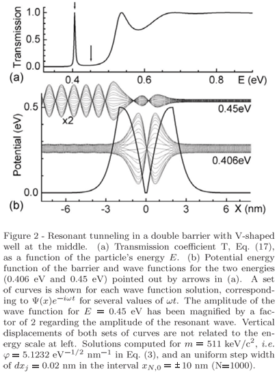
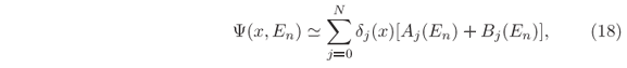
As an example, consider the potential given in Fig. 2, which is a double barrier with V-shaped well the middle. By scanning the energy values E, Eq. (3), in a chosen range from E_min to E_max in N_E steps of width dE so that E_n = E_min + (n-1)dE and = E_max, a T(E) curve is obtained as the one shown in Fig. 2(a). By storing the coefficients A_j(E_n) and B_j(E_n) when calculating the T values, high-resolution plots of the wave functions in the interval X also as a function of energy are already available, i.e.

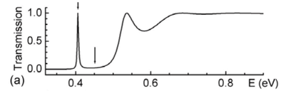
given that dx_j << l_j = 2p/|k_j|. Hence, amplitudes and attenuations of the waves through the entire barrier can be visualized. For this particular potential, it shows that the mode undergoing resonant-tunneling, at E = 0.406eV, has two maxima in the well as can be seen in Fig. 2(b).

Optionally one can compute only the R_j's and T_j's, Eq. (10), to obtain T = |T_j|² and either stop the calculation there if only the T(E) curve is desired or compute the A_j's and B_j's, Eqs. (9), later for a chosen set of energies. The options on how the present formalism can be programmed for optimizing computational tasks are detailed in ^{Appendix A}.

Although the stored set of solutions, Eq. (18), could be used to study the scattering of wave packets in the barriers, obtaining normalized wave packets would not be as straightforward as possible because the solutions are evenly spaced in energy, not in momentum. Therefore, if one wants to compute wave solutions only once, and also study wave packets composed of these solutions as well as their transmission coefficients, it is better to first define the form of the initial wave packet.

Gaussian wave packets has become a benchmark in computing time evolution of this sort [17], hence let use

as reference for our initial free-particle wave packet in t = 0, centered at x₀, and described by a single mode of energy E₀ so that k₀ = j. It is normalized since ò|Y(x,0)|²dx = 1, and its full width at half maximum (FWHM), W, can be chosen by providing s_x = W/@ 0.6 W.

Numerov-type solutions of the time-dependent SE can handled the time evolution of such wave packet, Eq. (19), through a given potential barrier [17], but in the present recursive method it is not possible to start with such expression of Y(x,0) since it is an artificial expression that happens to have the same shape, at t = 0, of the actual wave packet

where

and s_k = s_x^-1. For sake of normalization, the wave vectors k_n must be equally spaced, i.e. k_n+1-k_n = dk, so that

Since the c_n's out of the range k_n-k₀ = ±3.5s_k have negligible amplitude, the N_E modes with wave vectors k₁, k₂,..., are taken in this range to compose the wave packet, whose spectrum of energy is given by E_n = (k_n/j)². Energy difference between adjacent modes,

increases as n runs toward N_E. Hence, the maximum interval of time by which the evolution of the wave packet can be studied is

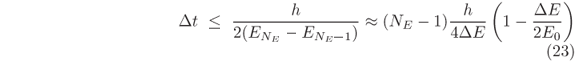
when the energy range E₀ ± DE comprises all E_n's.

To be more illustrative, let construct an initial guassian wave packet within a previously chosen range of energy, for instance, with E_n in the narrow range E₀ ± 0.058 eV around the energy E₀ = 0.406 eV of the resonant mode in Fig. 2. It leads to s_k @ jDE/7 = 0.0666 nm^-1 and to W = 25.0 nm as the FWHM of |Y(x,0)|². By composing the wave packet with 101 modes, our limit of time for studying its evolution is Dt < 1654fs, Eq. (23). Figure 3 shows the scattering process of such wave packet by the double barrier (Fig. 2) as computed via Eq. (20). The reflection of the entire wave packet occurs in a time interval no longer than 170fs, Fig. 3(a) through Fig. 3(c), but the resonant mode trapped in the well survives for much longer than that, Fig. 3(d). Its evanescence in time is dictated by an exponential decay of time constant of 184.5fs regarding the probability of finding the particle inside the well after t = 232.3fs, Fig. 3(c).

In case of potential with localized minima not reachable by tunneling from either sides, computing both left-hand and right-hand solutions is necessary. The procedure is very similar to the previous one used to obtain the Y(x,En) set of wave functions evenly spaced in energy where E_n+1-E_n = dE. But, most of these unilateral solutions do not exist under confinement. Hence, prior to calculate A_j's, B_j's, and T_j's from Eqs. (9) and (10a), we first compute the R_j's and _j's, Eqs. (10b) and (14b), to generate the f(E) plot according to Eq. (15). In Fig. 4(a) there are examples of such plot for a Lennard-Jones potential, a type of potential used to describe diatomic molecules and that has a single minimum. Only after providing an energy eigenvalue, _n, all other required coefficients for plotting the eigenfunction Y_n(x), Eq. (16), are calculated. For n = 1, 2, and 3, the eigenfunctions are shown in Fig. 4(b) where the one-dimensional variable x stands for the nuclei distance in the molecule. Although reduced mass, equilibrium distance, and ionization energy values are close of those for the H₂ molecule, the width of the depression in U(x) is much narrow than in the actual molecule [26]. It means a stronger restoring force and hence larger energy gaps in between adjacent vibrational states, which is used here for illustrative purposes only. In this hypothetical molecule, the non-constancy of the gap values is more evident, as can be seen in Fig. 4(a). It indicates how the exact solution would differ from the harmonic oscillator approximation.

Computational task involved in finding the energy eigenvalues E = _n in which f(E) = 0 can be enormous depending on number and accuracy of the desired eigenvalues. There will be no difficult in determining a few eigenvalues with reasonable accuracy, for instance ₁ = -3.4416 eV, ₂ = -1.8793 eV, ₃ = -0.8660 eV, and ₄ = -0.2991 eV in Fig. 4(a), are obtained at once in just a few seconds and with an accuracy of dE/2 = 0.0022 eV (N_E = 1000); x₀ = 0.002 nm, x_N = 0.2 nm, and dx_j = 0.0005 nm (N = 396). The problem relies in finding many eigenvalues, with high accuracy, occurring at different densities along a broad energy range. But practical needs of finding all possible eigenvalues are unusual, although it can be realized by developing search routines to reduce computational time since the method does not have any intrinsic limitation; as for instance the frequency distortion, or phase-lag, errors of the Numerov-type methods [12, 13].

Potential functions with singularities do not compromise the applicability of the presented method since only solutions with null wave functions at the singularities are those with physical meaning. In other words, when representing the potential by a discretized function, a finite value has to be assigned to the singularity. It compromises mostly the modes with non-null wave functions at the singularity, but these are artificial modes that do not exist in the actual physical system. Occurrence of artificial modes has been observed when solving the potential U(x) = -e²/[|x|+|e|] with e ® 0. In this case, the odd solutions with respect to the singularity provide the well-known eigenvalues of the hydrogen atom.

Another situation that can also be addressed by the recursive method occurs when the potential function has closely spaced minima, as for instance in the potential shown in Fig. 5. In the present formalism, the two minima (or wells) of this potential can be treated separately after establishing distinct intervals in X for calculating the function f(E). For each E_n Î [E_min,E_max], we first compute the R_j's and _j's in the entire interval X that contains the wells, i.e. from x₀ to x_N. Then, by selecting a position x_b somewhere in between the wells as indicated in Fig. 5(b), two f(E_n) values are obtained: one for x_j Î [x₀,x_b] and another for x_j Î [x_b+1,x_N], and always obeying that U(x_j) < E_n. Both f(E) curves thus obtained are shown in Fig. 5(a). As tunneling across the barrier separating the wells become relevant, the minima of the f(E) curves are coincidental. It means that the energy levels, or eigenvalues _n, in each well are independent from each other only if tunneling is negligible. It is more evident when visualizing the wave functions of the confined modes shown in Figs. 5(b), 5(c), and (d). In practice, potential with two minima are found for Cooper pairs (2 spin-coupled electrons) in Josephson-junction of superconducting materials [27].

In semiconductor heterostructures, the validity of this recursive method in its present formalism holds true when the charge carrier's effective mass can be approximated by a constant value through out the structure. However, accounting for effective mass variation across heterojunctions has only been possible in cases of abrupt interfaces and by using appropriated boundary conditions [28, 29].

Computing wave functions recursively is limited to problems treatable in one dimension, such as spherically symmetric potentials, or cases where the potentials in orthogonal directions are independent from each other, as for instance U(x,y) = U_X(x)+U_Y(y), in which the wave functions are obtained by the product of independent one-dimensional solutions. In all other cases of two and three dimensions, it is not possible to extend this recursive method since the number of unknown amplitude coefficients are more than the number of equations written by matching the wave function and its derivative at every steps of the discretized potentials. Hence only mathematical methods for solving 2D and 3D differential equations are available [3, 5, 29, 30].

4. Conclusions

This work has demonstrated that any one-dimensional quantum potential, wherever representing an open or closed system, can be solved by a single method and within good numerical accuracy. It is a simple tool ready to be used in applied physics or just in developing illustrative examples of quantum mechanics. It should also be emphasized that, in the presented formulation, the quantum potentials are solved by a physical treatment where the particle's wave function is molded by the same elemental action of the given force field. This is a completely different approach of the one that is usually taken where, once the potential is known, the problem became the mathematical solution of a differential equation.

Acknowledgments

During the time dedicated to this work, financial supports were received from CNPq (301617/1995-3 and 304916/2006-4), FAPESP (2002/10387-5), and CAPES-GRICES (140/05).

Recebido em 28/11/2006; Aceito em 8/5/2007

There are several ways to program the recursive formalism presented in this work, depending on what information is desired. The flowchart in Fig. 6 describes the basic structure of the routines used to elaborate the examples in Figs. 2 to 5. Once the U(x) function and the discretization of X is defined, the user can choose either route or to scan a given energy range in fixed increments of energy, dE, or wavevector, dk, respectively. The latter route is suitable to study time evolution of wave packets by ending through route , i.e. 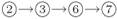. Eigenvalues {₁, ₂,...}, of confined modes are obtained from the f(E) curve in route , and used as input to provide the eigenfunctions Y_n(x) through route . The straight route are exclusive for users interested only in transmission coefficients across arbitrary potential barriers.

• [1] D.R. Hartree, The Calculation of Atomic Structures (Pergamon, London, 1957).
• [2] D. Bohm, Quantum Theory (Dover, New York, 1989).
• [3] C.S. Lent and D.J. Kirkner, J. Appl. Phys. 67, 6353 (1990).
• [4] A.R. Lee and T.M. Kalotas, Phys. Scr. 44, 313 (1991).
• [5] H.W. Jang and J.C. Light, J. Chem. Phys. 102, 3262 (1995).
• [6] T.E. Simos, Computers Math. Applic. 33, 67 (1997).
• [7] N.C. Kluksdahl, A.M. Kriman, D.K. Ferry and C. Ringhofer, Phys. Rev. B 39, 7720 (1989).
• [8] W.R. Frensley, Rev. Mod. Phys. 62, 745 (1990).
• [9] T.B. Boykin and G. Klimeck, Eur. J. Phys. 25, 503 (2004).
• [10] N.B. Abdallah and O. Pinaud, J. Comput. Phys. 213, 288 (2006).
• [11] M. Dehghan, Math. Comput. Simul. 71, 16 (2006).
• [12] T.E. Simos and G. Tougelides, Computers Chem. 20, 397 (1996).
• [13] T.E. Simos and P.S. Williams, Computers Chem. 25, 77 (2001).
• [14] H. Van der Vyver, Appl. Math. Comput. 171, 1025 (2005).
• [15] S.A. Chin and P. Anisimov, J. Chem. Phys. 124, 054106 (2006).
• [16] V. Ledoux, M. van Daele and G. vanden Berghe, ACM Trans. Math. Softw. 31, 532 (2005).
• [17] C.A. Moyer, Am. J. Phys. 72, 351 (2004).
• [18] S.A. Shakir, Am. J. Phys. 52, 845 (1984).
• [19] T.M. Kalotas and A.R. Lee, Am. J. Phys. 59, 48 (1991).
• [20] T.M. Kalotas and A.R. Lee, Am. J. Phys. 59, 1036 (1991).
• [21] P. Senn, Am. J. Phys. 60, 776 (1992).
• [22] S.K. Biswas, L.J. Schowalter, Y.J. Jung, A. Vijayaraghavan, P.M. Ajayan and R. Vajtai, Appl. Phys. Lett. 86, 183101 (2005).
• [23] A. Zhang, Z. Cao, Q. Shen, X. Dou and Y. Chen, J. Phys. A: Math. Gen. 33, 5449 (2000).
• [24] C.V.-B. Tribuzy, S.M. Landi, M.P. Pires, R. Butendeich and P.L. Souza, Brazilian J. Phys. 32, 269 (2002).
• [25] Q.S. Zhu, Z.T. Zhong, L.W. Lu and C.F. Li, Appl. Phys. Lett. 65, 2425 (1994).
• [26] Y.K. Syrkin and M.E. Dyatkina, Structure of Molecules and the Chemical Bond (Interscience Publishers, Nova Iorque, 1950).
• [27] D.B. Josephson, Rev. Mod. Phys. 46, 251 (1974).
• [28] G. Bastard, Wave Mechanics Applied to Seminconductor Heterostructures (John Wiley and Sons, Nova Iorque, 1991).
• [29] J. Wang, E. Polizzi and M. Lundstrom, J. Appl. Phys. 96, 2192 (2004).
• [30] T.-M. Hwang, W.-W. Lin, W.-C. Wang and W. Wang, J. Comput. Phys. 196, 208 (2004).

Appendix A

Publication Dates

• Publication in this collection
  07 Dec 2007
• Date of issue
  2007

History

• Accepted
  08 May 2007
• Received
  28 Nov 2006