Introduction to continuous photocounting effects on the quantized optical field

Abstract

In this manuscript, we explore the effects of continuous measurements upon the quantized electromagnetic field through a series of simple examples. For this purpose, we consider the Srinivas-Davies model to describe the optical field dynamics probed continuously by a photodetector. Through the application of this continuous photodetection model to some specific situations, it is possible to cover some basic concepts of quantum mechanics such as the principle of superposition, the collapse of the wave function, the probabilistic character of the possible outcomes associated with projective measurements, as well as some advanced topics such as the description of open quantum systems, irreversible processes in quantum mechanics, decoherence and dissipation associated with non-unitary evolution of quantum systems. Besides, we also consider the important concept of entanglement between two electromagnetic fields and how it is affected by the photodetection process. This work aims to provide complementary material for undergraduate and graduate students interested in the effects of measuring devices acting on quantum systems.

Keywords:
Continuous measurements; Photodetection; Quantized optical fields

1. Introduction

The postulates of Quantum Mechanics (QM), following the Copenhagen interpretation, establish the foundations to describe nature at the microscopic scale. Inside the QM formalism, it is possible to describe atoms, molecules as well as light and their mutual interactions [1,2]. Since the birth of QM, the investigations about coherence, quantum dynamics, projective measurements, and the intrinsic probabilistic nature of the outcomes associated with these kinds of measurement, are extremely important to check the veracity of the postulates and, therefore, of great interest to physicists concerned about the foundations of QM. Until now there is no experimental evidence that demonstrates any inconsistency with the postulates or the Copenhagen interpretation of QM [3 -5].

In this paper, we are interested in exploring the concepts raised above, considering continuous measurements applied to the quantized optical field via photodetection. Despite an extensive literature [6 -15] about this subject, we care about being quite pedagogical to help advanced undergraduate and graduate students interested in the effects of measuring devices acting on quantum systems. This kind of problem is becoming increasingly important given the significant quantum-based technologies advancements [16 -31].

To take into account the action of the detector on the optical field, we use the theoretical photodetection model developed by Srinivas and Davies [6,8,15]. The Srinivas-Davies model is based on the mathematical framework called quantum operations [16] which permits not only to calculate the evolution of closed systems but also the evolution of open quantum systems. It is important to learn and dominate techniques that describe the dynamics of quantum systems interacting with the environment since in real life there is no such thing as closed system, and to describe real processes we have to take into account the influence of the rest of the Universe upon the system of interest.

The Srinivas-Davies model is presented in Sec. 2. In Sec. 3, to illustrate basic and general results, we review the simplest case where the Srinivas-Davies model can be applied: just one-mode of the optical field. For an arbitrary initial state, we not only present the dynamics of the field probed by the detector (the conditioned and unconditioned states) and the photocounting probability distribution (the probability distribution associated with the number of photons counted by the detector over a time period t), but we also present detailed calculations. For concreteness, we review two specific cases, the number and the coherent states, pointing out the differences and the similarities between them when they are probed by a photodetector. In Sec. 4, we consider another example given by a superposition of two coherent states and analyze the dependence on the number of photons counted upon the dynamics of two special cases: the odd and even superpositions of coherent states. In Sec. 5, we consider two non-interacting optical fields initially prepared as an entangled state of two-mode coherent states. There we assume two scenarios: one in which just one mode is continuously probed, showing how the combined state evolves under the influence of a local detection, and another where both modes are probed by two independent photodetectors with different detection rates. In order to guide the readers, the calculations needed to obtain the main results concerning the dynamics of the probability distributions and the conditioned and unconditioned states are detailed in the appendices. Finally, in Sec. 6 a summary is presented.

2. Srinivas-Davies continuous photocounting model

The Srinivas-Davies continuous photocounting model (SD-model) is based on the following statement: whenever a system in an arbitrary state ρ is subject to a process (instantaneous or not) and a certain outcome is observed as a result, the state that emerges from the process will be of the form [16]

(1) $$\frac{ϵ\rho }{\mathrm{T}\mathrm{r}\left[ϵ\rho \right]}.$$

The operator ρ is the density operator, also known as the statistical operator, and it represents the physical state of the system [1,2,32]. The map ε in the equation (1) is what is called a quantum operation; it can represent an unitary evolution of a closed system, the collapse of a state due to a measurement associated with some observable, a non-unitary evolution of a system interacting with the environment, or a more general process that encompasses non-unitary evolution between multiple instantaneous projective measurements. In mathematical language, just for the sake of formality, an operation ε is a linear positive transformation on the space of all trace class operators on the Hilbert space $\mathcal{H}$, such that $0\le \mathrm{T}\mathrm{r}[ϵ\rho ]\le 1$ (for each normalized density operator ρ), where $\mathrm{T}\mathrm{r}[ϵ\rho ]$ is the probability that the outcome corresponding to ε has been observed.

Another mathematical particularity that we consider relevant to mention is that the SD-model satisfies a semi-group structure which means that the dynamics of the system is irreversible in time. A semi-group is an algebraic structure that requires only the associative property between the elements of a set provided with a binary operation rule, and it does not need to have the identity nor the inverse operations. Furthermore, if the system in the state ρ is subject to a sequence of two experiments with outcomes corresponding to the operations ${ϵ}_1$ and ${ϵ}_2$ respectively, then the state of the system just after the second experiment will be

(2) $$\frac{{ϵ}_2{ϵ}_1\rho }{\mathrm{T}\mathrm{r}\left[{ϵ}_2{ϵ}_1\rho \right]},$$

with $\mathrm{T}\mathrm{r}\left[{ϵ}_2{ϵ}_1\rho \right]$ being the joint probability that the above sequence of outcomes happens. In other words, the maps that define the semi-group dynamics in the SD-model are what is known in the literature as divisible maps [33 -35].

Here, we are interested in describing the action of the photodetection on a quantized electromagnetic field. In this context, the process of photodetection represented by the SD-model is characterized by a set of operations $N_{[t,t+\tau )}\left(k\right)$ which define the conditioned state

(3) $$\frac{N_{[t,t+\tau )}\left(k\right)\rho }{\mathrm{T}\mathrm{r}\left[N_{[t,t+\tau )}\left(k\right)\rho \right]}.$$

The state above is the evolved state conditioned to the number k of photons counted by the detector over a time interval $[t,t+\tau )$, where ρ represents the initial state of the quantized optical field. As we will see in the next sections, the initial state of the quantized electromagnetic field can be represented by a number of possibilities. Each representation of the initial state is associated to a particular probability distribution which corresponds to a signature of the optical field that can be obtained experimentally by photodetection. Also, the conditioned state given by equation (3) depends on the initial state and the type of photodetection process, which is usually accomplished by photon absorption. The state given by equation (3) represents the change of the optical field due to its coupling with the detector. Hereafter, we adopt (as Srinivas and Davies did in their seminal paper [6]) only homogeneous counting processes for which $N_{[t,t+\tau )}\left(k\right)$ are independent of the initial time, that is

(4) $$N_{[t,t+\tau )}\left(k\right)=N_{\tau }\left(k\right),$$

depending only on the time interval $\tau$. Homogeneous counting processes can be characterized by some axioms that are related with the probabilistic character of

(5) $$\text{Pr}(k,t)=\mathrm{T}\mathrm{r}\left[N_t\left(k\right)\rho \right]$$

which is the probability of the event “k photons counted by the detector during the time lapse t”. These axioms are the following: $0\le \mathrm{T}\mathrm{r}\left[N_t\left(k\right)\rho \right]\le 1$ ensures that $\text{Pr}(k,t)$ assumes values inside the interval $[0,1]$; the operation $T_t=\sum _{k=0}^{\mathrm{\infty }}{N}_t\left(k\right)$ satisfies $\mathrm{T}\mathrm{r}\left[T_t\rho \right]=1$ since $\sum _{k=0}^{\mathrm{\infty }}\text{Pr}(k,t)=1$; $N_{t_1+t_2}\left(k\right)=\sum _{k_1+k_2=k}{N}_{t_2}\left(k_2\right)N_{t_1}\left(k_1\right)$ relates the joint probability $\text{Pr}(k_1,[0,t_1);k_2,[t_1,t_2))$ that $k_1$ photocounting is recorded in the interval $[0,t_1)$ and $k_2$ in the interval $[t_1,t_1+t_2)$, where the probability that $k=k_1+k_2$ photons are recorded during the total time interval $t=t_1+t_2$ is given by $\text{Pr}(k,[0,t_1+t_2))=\sum _{k_1+k_2=k}\text{Pr}(k_1,[0,t_1);k_2[t_1,t_2))$. Besides,

(6) $$\underset{t\to 0}{lim}{N}_t(0)\rho =\rho$$

ensures that

(7) $$\underset{t\to 0}{lim}\text{Pr}(0,t)=1,$$

i.e., the probability of the detector records a photocounting at the very beginning of time is extremely unlikely and it goes to zero in the limit $t\to 0$.

The operation $N_t(k)$ is given in terms of two fundamental operations which completely characterize the photocounting process within the SD-model. The operation $S_t$ is one of them and it represents the non unitary evolution that the optical field undergoes between two consecutive photodetections. Following [6] we assume that

(8) $$S_t\rho =e^{Yt}\rho e^{Y^{†}t},$$

where Y is the generator of the semi-group dynamics given by divisible maps $S_t\rho =S_{t_2}{S}_{t_1}\rho$, where $t=t_1+t_2$. The other operation that composes $N_t(k)$ is J and it is responsible for the instantaneous absorption of a photon from the optical field by the detector, that is, the operation J is responsible for the collapse of the state of the field into a state having minus one photon. It is assumed by the SD-model that the detector cannot count two or more photons at the same time. Mathematically we can write this assumption as follows

(9) $$\underset{t\to 0}{lim}\frac{N_t(k)\rho }{t}=0\text{for}k\ge 2$$

with

(10) $$\underset{t\to 0}{lim}\frac{N_t(1)\rho }{t}=J\rho .$$

In terms of the operations $S_t$ and J, $N_t(k)$ is given by

(11) $$\begin{array}{rcl}& & N_t\left(k\right)\rho ={\int }_0^{t}d{t}_k{\int }_0^{t_k}d{t}_{k-1}\dots \\ & & {\int }_0^{t_2}d{t}_1{S}_{t-t_k}J{S}_{t_k-t_{k-1}}\dots J{S}_{t_1}\rho .\end{array}$$

Since the operation $S_t$ is divisible, the integrand in the equation (11) can be rewritten as follows

(12) $$\begin{array}{rcl}& & N_t\left(k\right)\rho ={\int }_0^{t}d{t}_k{\int }_0^{t_k}d{t}_{k-1}\dots \\ & & {\int }_0^{t_2}d{t}_1{S}_{t}J(t_k)J(t_{k-1})\dots J(t_1)\rho ,\end{array}$$

where

(13) $$J(t_j)\rho =S_{-t_j}J{S}_{t_j}\rho .$$

Considering a canonical photoncounting process, where the operation $S_t$ is completely defined by the operation J, the generator Y is given by

(14) $$Y=-i\frac{H}{\hslash }-\frac{R}{2},$$

where the Hilbert space operator R is defined by

(15) $$\mathrm{T}\mathrm{r}\left[\rho R\right]=\mathrm{T}\mathrm{r}\left[J\rho \right].$$

These choices given by equations (8), (14) and (15) reflect the complementary property of the two mutually exclusive probabilities

(16) $$P(J)\tau +P(S_{\tau })=1,$$

that is, the complementarity between the probability associated to the event “to count 1 photon during an infinitesimal interval of time $\tau$” ($P(J)\tau$) and the probability associated with the event “not to count 1 photon during the same interval of time” ($P(S_t)$).

The probability $P(J)\tau =\mathrm{T}\mathrm{r}\left[J\rho \right]\tau$ is dimensionless since $J\rho$ is given by the equation (10) which has the dimension of frequency. The probability $P(S_{\tau })=\mathrm{T}\mathrm{r}\left[S_t\rho \right]$ is also dimensionless since ideally $S_{\tau }\rho =N_{\tau }\left(0\right)\rho$. When equation (8) is satisfied, the equation (16) is completely equivalent to the following relation (see Appendix A):

(17) $$\mathrm{T}\mathrm{r}\left[\rho R\right]=\mathrm{T}\mathrm{r}\left[J\rho \right]=-\mathrm{T}\mathrm{r}[Y\rho +\rho Y^{†}].$$

3. Single-mode free field photocounting statistics

In this section we consider the formalism developed by Srinivas and Davies applied to the simplest possible case: one-mode of the quantized electromagnetic field. Although this example is found in the original Srinivas and Davies paper [6], we include it here for the sake of completeness, containing further discussions illustrating the results and the basic techniques that will be useful in the following sections. The evolution of such system is generated by the Hamiltonian [36]

(18) $$H=\hslash \omega a^{†}a,$$

where $\omega$ is the natural angular frequency of oscillation of the field, $\hslash$ is the Plank's constant divided by $2\pi$, and the operators $a^{†}$ and a are the photon creation and annihilation operators, respectively. These operators satisfy the usual bosonic commutation relation $[a,a^{†}]=1$. If $\{|n⟩\}$ denotes the basis composed of the eigenvectors of the Hamiltonian (18), known as the Fock (or Number) states, then $a^{†}$ and a satisfy the following relations

(19) $$a|n⟩=\sqrt{n}|n-1⟩,$$

(20) $$a^{†}|n⟩=\sqrt{n+1}|n+1⟩,$$

which naturally implies that

(21) $$N|n⟩=a^{†}a|n⟩=n|n⟩.$$

Clearly, from equation (19), the role of the annihilation operator is to remove a quantum of light from the field changing its state from one with n photons to another with $n-1$ photons. The creation operator has the opposite role.

The number operator $N=a^{†}a$, whose eigenvalues are formed by non-negative integers, gives the number of photons contained in the optical field. Since $[H,N]=0$, the number operator is a constant of motion. The meaning of this is simple: considering a closed system governed by the Hamiltonian (18), i.e., considering one-mode of electromagnetic field evolving freely in the absence of a detector (or any other process that can remove photons from the field) and in the absence of a pump laser (or any other process that can introduce photons into the field), the number of photons is, obviously, constant. Because the pair of observables commutes they are called compatible observables in the sense that the result of measuring one of them has no effect on the result of measuring the other and they can be measured simultaneously [1]. Besides, the Fock basis diagonalizes simultaneously both observables, that is, the Hamiltonian and the number operator share the same set of eigenvectors. Moreover, this set of vectors form a complete and orthogonal set:

(22) $$\sum _{n=0}^{\mathrm{\infty }}|n⟩⟨n|=1,$$

(23) $$⟨m|n⟩={\delta }_{mn}.$$

Naturally, we can express the most general one-mode optical field state as follows

(24) $$\rho =\sum _{m,n=0}^{\mathrm{\infty }}{\rho }_{mn}|m⟩⟨n|,$$

where ${\rho }_{mn}$ can be either a statistical weight (and in this case the state is a statistical mixture of Fock states) or a pure state with ${\rho }_{mn}=c_m{c}_n^{\ast }$, where $c_m=⟨m|\psi ⟩$ are the probability amplitudes and the state of the system is written as a linear combination of Fock states: $|\psi ⟩=\sum _n{c}_n|n⟩$.

Now, if we consider a detector probing the optical field, every time that one photon is detected (by absorption) the field loses that photon to the detector. To represent this absorption process mathematically it is reasonable to write the super operator J through the following expression

(25) $$J\rho =\gamma a\rho a^{†},$$

where γ is a parameter related with the detector's efficiency and represents the coupling between the detector and the field. A microscopic model for a detector operating by photon absorption justifying the choice in the equation (25) can be found in [10]. The equation (25) implies via equation (15) that

(26) $$R=\gamma a^{†}a.$$

Then, the generator of the non-unitary dynamics in which the single-mode optical field is subject between two consecutive photocountings is given by

(27) $$Y=-i(\omega -i\frac{\gamma }{2})a^{†}a.$$

Besides, from the equations (25) and (13) we have

(28) $$\begin{array}{rcl}& & J(t_j)\rho =S_{-t_j}J{S}_{t_j}\rho =\gamma e^{-Y{t}_j}a{e}^{Y{t}_j}\rho e^{Y^{†}{t}_j}{a}^{†}{e}^{-Y^{†}{t}_j}\\ & & =\gamma a(t_j)\rho a^{†}(t_j),\end{array}$$

where

(29) $$a(t_j)=e^{-Y{t}_j}a{e}^{Y{t}_j}$$

(30) $$a^{†}(t_j)=e^{Y^{†}{t}_j}{a}^{†}{e}^{-Y^{†}{t}_j},$$

which implies that

(31) $$\begin{array}{rcl}& & N_t\left(k\right)\rho ={\gamma }^k{S}_t{\int }_0^{t}d{t}_k\dots \\ & & {\int }_0^{t_2}d{t}_{1}a(t_k)\dots a(t_1)\rho a^{†}(t_1)\dots a^{†}(t_k).\end{array}$$

With the help of the following theorem (see [36]): If A and B are two non-commuting operators and ξ an arbitrary parameter, then

(32) $$\begin{array}{rcl}& & e^{\xi A}B{e}^{-\xi A}=B+\xi [A,B]+\frac{{\xi }^2}{2!}[A,[A,B]]\\ & & +\frac{{\xi }^3}{3!}[A,[A,[A,B]]]+\dots ,\end{array}$$

it is possible to calculate the equations (29) and (30), which gives:

(33) $$a(t_j)=a{e}^{{}^{-i(\omega -i\frac{\gamma }{2})t_j}}$$

(34) $$a^{†}(t_j)=a^{†}{e}^{{}^{i(\omega +i\frac{\gamma }{2})t_j}}.$$

With the equations (33) and (34), the operation (31) becomes

(35) $$N_t\left(k\right)\rho =S_t{J}^k\rho {\int }_0^{t}d{t}_k\dots {\int }_0^{t_2}d{t}_1{e}^{-\gamma (t_1+t_2+\cdots +t_k)}.$$

The calculus of the multiple integral above is presented in the Appendix B which gives the following result

(36) $${\int }_0^{t}d{t}_k{\int }_0^{t_k}d{t}_{k-1}...{\int }_0^{t_2}d{t}_1{e}^{{}^{-\gamma (t_1+t_2+...t_k)}}=\frac{{(1-e^{-\gamma t})}^k}{{\gamma }^{k}k!}.$$

Therefore, the state (3) and the probability distribution (5) in terms of the fundamental operations J (which absorves one photon from the field by the detector) and $S_t$ (which evolves non-unitarily the state of the field between two photocountings) become

(37) $${\rho }^{\left(k\right)}(t)=\frac{S_t{J}^k\rho \left(0\right)}{Tr\left[S_t{J}^k\rho \left(0\right)\right]},$$

(38) $$Pr(k,t)=\mathrm{T}\mathrm{r}\left[S_t{J}^k\rho \left(0\right)\right]\frac{{(1-e^{-\gamma t})}^k}{{\gamma }^{k}k!}.$$

The state (37) is obtained after k photons have been detected by the measuring device during the probing time t. It represents our knowledge about the optical field state after the continuous photodetection process has ended. It is called conditioned state since it is conditioned to (our knowledge about) the number of photons that were counted. Now, if we want to know how likely is this particular outcome, that is, if we want to know how probable is to count k photons during the probing time t, the answer is given by the equation (38). Considering an initial state of the form (24), the probability (38) can be written as follows

(39) $$Pr(k,t)=\sum _{m=k}^{\mathrm{\infty }}\left(\begin{array}{c}m\\ k\end{array}\right){(1-e^{-\gamma t})}^k{\left(e^{-\gamma t}\right)}^{m-k}{\rho }_{mm}\left(0\right),$$

where $\left(\begin{array}{c}m\\ k\end{array}\right)=\frac{m!}{k!(m-k)!}$ is the binomial coefficient. Both expressions, (38) and (39), show that the probability distribution $Pr(k,t)$ is strongly dependent on the initial state of the system and both represent general and equivalent expressions for the one-mode optical field photocounting probability distribution. Identical formulas to equation (39) were obtained before the Srinivas-Davies theory in Refs. [37] and [38] using other approaches.

As we can see in the equation (39), for $\gamma t\gg 1$ (which means either a large period of probing time or a fast detection rate or both) only the first term in the sum remains and the photocounting probability distribution $Pr(k,t)$ reproduces (asymptotically) the initial state probability distribution $P_n=⟨n|\rho \left(0\right)|n⟩={\rho }_{nn}\left(0\right)$, i.e.,

(40) $$\underset{\gamma t\to \mathrm{\infty }}{lim}Pr(k,t)\sim {\rho }_{kk}\left(0\right).$$

The conditioned state (37) is the state that emerges from the continuous photodetection process when it is known how many photons were counted during the probing time t; however, if it is not known how many photons were counted during the probing time we usually describe our lack of information about the state through the unconditioned state, which is the state obtained averaging the conditioned state (37) over all possible k counts weighted by the photocouting probability distribution (39)

(41) $$\rho \left(t\right)=\sum _{k=0}^{\mathrm{\infty }}Pr(k,t){\rho }^{\left(k\right)}\left(t\right).$$

The equations (37), (39) and (41) can be applied for any initial one-mode optical field state. Let us then illustrate the applicability of these equations for some concrete examples. Let us begin with two well known particular cases, the number and the coherent states [8,36,39].

In the first example, if we prepare the initial optical field in a state where we know for sure how many photons are contained initially in the field, that is, a number state $|n_0⟩$, which implies to choose ${\rho }_{mn}\left(0\right)={\delta }_{m{n}_0}{\delta }_{n{n}_0}$ where $n_0$ is the number of photons contained in the field at $t=0$, then equations (37), (39) and (41) give us the following dynamics for the conditioned state, the photocounting probability distribution and the unconditioned state, respectively:

(42) $${\rho }^{\left(k\right)}\left(t\right)=|n_0-k⟩⟨n_0-k|,$$

(43) $$Pr(k,t)=\left(\begin{array}{c}{n}_0\\ k\end{array}\right){(1-e^{-\gamma t})}^k{\left(e^{-\gamma t}\right)}^{n_0-k},$$

and

(44) $$\rho \left(t\right)=\sum _{k=0}^{\mathrm{\infty }}\left(\begin{array}{c}{n}_0\\ k\end{array}\right){(1-e^{-\gamma t})}^k{\left(e^{-\gamma t}\right)}^{n_0-k}|n_0-k⟩⟨n_0-k|.$$

What can we conclude from the conditioned and unconditioned states (42) and (44)? And what can we say about the probability distribution (43)? First of all, we can see that the conditioned state (42) does not depend on time at all, depending solely on the number of photons counted by the detector. It represents the collapse of the initial state $|n_0⟩$ into the final state $|n_0-k⟩$, after k photons have been detected, which is the state that emerges from the photocounting process if we know how many photons were counted. Obviously, although the state (42) does not depend on time, the odds of a particular event is time dependent and is given by the probability distribution (43). The time dependent probabilities $Pr(k,t)$ for $k=0,1,2,\dots ,10$ with $n_0=10$ and $\gamma =1$ are depicted in different colours in the Fig. 1.

Figure 1
The time dependence of the photocounting probability distribution $Pr(k,t)$ given by the equation (43) for different values of k when the initial state is the number state $|n_0⟩$. Here we choose $n_0=10$ and $\gamma =1$.

As we can see in the Fig. 1, each possible outcome has its own time dependent probability distribution $Pr(k,t)$. For instance, the probability to count no photons $Pr(0,t)=e^{-\gamma n_{0}t}$ is initially equal to 1 and decays exponentially to 0 as a function of time. For $0<k<10$ the probabilities reach a maximum value for some intermediate time and then also decay asymptotically to 0 for large times. As may be expected, the time scale is defined by the detector's efficiency γ and by the initial number of photons in the field $n_0$. For $k=10$, which corresponds to the event of count all the photons available in the initial field, the probability $Pr(10,t)={(1-e^{-\gamma t})}^{10}$ increases monotonically with time from 0 to 1 indicating that for sufficiently long time all the photons in the field are counted leaving the field in the vacuum state $|0⟩⟨0|$.

Now, let us suppose that it is not known how many photons were counted during the process. Let us say that, for some reason, we only know that the detector has counted some number of photons but we do not know that number. In this case, we are unable to say what the optical field state is for sure but, instead, we could say that the state of the field can be $|n_0⟩⟨n_0|$ with probability $Pr(0,t)$, or can be $|n_0-1⟩⟨n_0-1|$ with probability $Pr(1,t)$, and so on. In this situation, the state of the field is in a statistical mixture of pure states (42) weighted by the probabilities (43), which is well represented by the unconditioned state (44). This state is a mixed state and the statistical matrix that represents the density operator (44) is a diagonal matrix with null non-diagonal elements.

The second example of a single-mode initial state considered in this section is the coherent state [39]. This important representation of the optical field can be written as an infinity superposition of Fock states [36],

(45) $$|\alpha ⟩=e^{-|\alpha {|}^2/2}\sum _{n=0}^{\mathrm{\infty }}\frac{{\alpha }^n}{n!}|n⟩.$$

The photon number probability distribution for the coherent state follows a Poisson distribution

(46) $$P_n=|⟨n|\alpha ⟩{|}^2=⟨n|\alpha ⟩⟨\alpha |n⟩=e^{-{\left|\alpha \right|}^2}\frac{|\alpha {|}^{2n}}{n!},$$

with an average number of photons given by $⟨n⟩=⟨\alpha |a^{†}a|\alpha ⟩=|\alpha {|}^2$. Unlike the number state which has a definite number of photons and, consequently, a maximal uncertainty on its phase, the coherent state has a definite phase with an indefinite number of photons.

From the equations (45) and (24) we have ${\rho }_{mn}=e^{-{\left|\alpha \right|}^2}\frac{{\alpha }^m{\left({\alpha }^{\ast }\right)}^n}{\sqrt{m!n!}}$ for the coherent state. Then the conditioned state (37) and the photocounting probability distribution (39) are, respectively, given by (see Appendix C for details)

(47) $${\rho }^{\left(k\right)}\left(t\right)=|\alpha e^{-i(\omega -i\frac{\gamma }{2})t}⟩⟨\alpha e^{-i(\omega -i\frac{\gamma }{2})t}|,$$

(48) $$Pr(k,t)=e^{-{\left|\alpha \right|}^2}\sum _{m=k}^{\mathrm{\infty }}\left(\begin{array}{c}m\\ k\end{array}\right){(1-e^{-\gamma t})}^k{\left(e^{-\gamma t}\right)}^{m-k}\frac{|\alpha {|}^{2m}}{m!},$$

where the sum in the equation (48) converges to the following expression (see Appendix D)

(49) $$Pr(k,t)=\frac{({\left|\alpha \right|}^2-{|\alpha (t)|}^2{)}^k}{k!}{e}^{-({\left|\alpha \right|}^2-{|\alpha (t)|}^2)},$$

with $\alpha (t)=\alpha e^{-i(\omega -i\frac{\gamma }{2})t}$.

It is interesting to notice that the coherent state is not affected by the operation J during the photocounting process since it is an eigenvector of the annihilation operator,

(50) $$a|\alpha ⟩=\alpha |\alpha ⟩,$$

with complex eigenvalue $\alpha =\left|\alpha \right|e^{i\varphi }$. Consequently, the conditioned state (47) does not depend on k. On the other hand, between two successive photocountings the operation $S_t$ induces two effects over the coherent state: a time dependent phase shift due to the free evolution of the field and an irreversible amplitude exponential decay due to the non-unitary part of the evolution. Therefore, the coherent state remains coherent during the whole photocounting process decreasing its amplitude continuously until all the photons in the field have been detected and the original field has reached its final state, i.e., the vacuum state (which is a coherent state as well). Moreover, since the conditioned state dynamics (47) is independent of k and $\sum _{k=0}^{\mathrm{\infty }}Pr(k,t)=1$, the unconditioned state (41) and the conditioned state are the same:

(51) $$\rho (t)=|\alpha (t)⟩⟨\alpha (t)|.$$

Hence, it does not matter if one knows or not how many photons are counted during the photocounting process, the coherent state will remain pure and coherent all the time, differently from the number state where the lack of information about how many photons are counted is manifested as a mixed state with statistical weights, as expressed by equation (44).

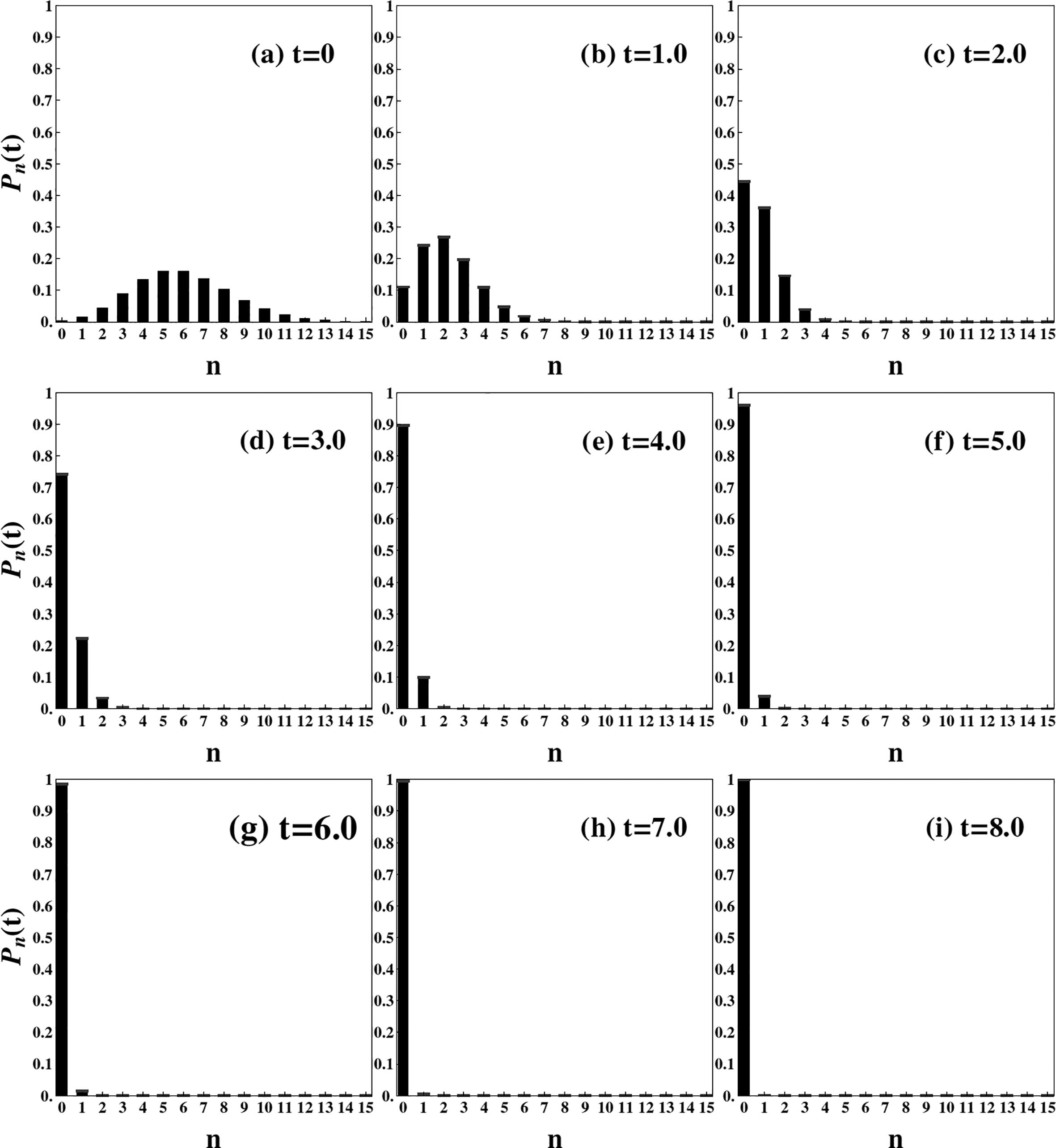
The photon number probability distribution associated with the evolved state of the field, $P_n(t)=|⟨n|\alpha (t)⟩{|}^2=⟨n|\alpha (t)⟩⟨\alpha (t)|n⟩$, is a time dependent Poisson distribution

(52) $$P_n(t)=e^{-{|\alpha (t)|}^2}\frac{|\alpha (t){|}^{2n}}{n!}.$$

Figure (2) shows the photon number probability distribution dynamics given by the equation (52) for different times and for $⟨n⟩=|\alpha {|}^2=6$ and $\gamma =1$. At the initial time $t=0$ the photon number probability distribution $P_n(t)$ given by the equation (52) is identical to $P_n$ given by the equation (46), which can be seen in the Fig. (2)-(a). Figures from (2)-(b) to (2)-(h) show that the distribution $P_n(t)$ moves from right to left as the amplitude of the field decreases with time due to the non-unitary action of the detector. It means that asymptotically all the photons of the field will be counted and the only probability that survives is $P_0(\mathrm{\infty })=1$ [see Fig. (2)-(i)] indicating that the conditioned state given by equation (51) reaches the vacuum state for a long enough time

Figure 2
The photon number probability distribution $P_n(t)$ given by the equation (52) for the initial coherent state $|\alpha ⟩$ for different times. We set $|\alpha {|}^2=6$ and $\gamma =1$. In (a)$t=0$; (b)$t=1.0$; (c)$t=2.0$; (d)$t=3.0$; (e)$t=4.0$; (f)$t=5.0$; (g)$t=6.0$; (h)$t=7.0$; (i)$t=8.0$. Time is in units of $1/\gamma$.

(53) $$\underset{t\to \mathrm{\infty }}{lim}\rho (t)=\underset{t\to \mathrm{\infty }}{lim}|\alpha (t)⟩⟨\alpha (t)|=|0⟩⟨0|.$$

The photodetection probability distribution given by equation (49) is depicted in the Fig. (3) for the same average number of photons $|\alpha {|}^2=6$ and the same detection rate $\gamma =1$ considered in the Fig. (2). As it can be observed, the behaviour of the photocouting probability distribution $Pr(k,t)$ given by equation (49) is the opposite observed for the photon number distribution in the equation (52). Initially the photocounting probability $Pr(k,t)$ to count $k=0$ is the only non null probability and it is equal to 1 [see Fig. (3)-(a)]. In the course of time, the photocounting probability distribution given by the equation (49) moves from left to right [see Figs. from (3)-b to (3)-k] and for long enough time it reproduces the initial probability distribution of the optical field given by equation (46) [see Fig. (3)-l] as expected from the equation (40). The opposite behaviors observed between the photon number probability distribution and the photodetection probability distribution is in agreement with the law of energy conservation which states that the total energy of an isolated system (field + detector) remains constant over time.

Figure 3
The photocounting probability distribution $Pr(k,t)$ given by the equation (49) for the initial coherent state $|\alpha ⟩$ with $|\alpha {|}^2=6$ and $\gamma =1$. In (a)$t=0$; (b)$t=0.1$; (c)$t=0.2$; (d)$t=0.3$; (e)$t=0.4$; (f)$t=0.5$; (g)$t=0.6$; (h)$t=0.7$; (i)$t=0.8$; (j)$t=0.9$; (k)$t=1$; (l)$t=5$. Time is in units of $1/\gamma$.

From an experimental point of view, the optical field intensities (or even individual photons) are not measured directly but rather indirectly, measuring the photocurrent produced and amplified by the detector. The photocurrent statistics reflects the statistical properties of light. For a better understanding of the photodetection process in real experiments let us consider the simplest optical setup needed to measure photon statistics. This setup needs three basic devices: a source of light, a photodetector and a discriminator. The source of light can be a hight-quantum-efficiency light emitting diode (LED), which is suited for the producing of a quantized light beam. A good photodetector candidate which is well-suited for laboratory applications, enabling individual photons to be detected when the incident flux of light is low and the optical field needs to be treated quantum mechanically, are the photomultiplier tubes (PMTs), which are photodetectors that absorves and transforms incident photons, via photoelectric effect, into measurable electric pulses (the photocurrents). Basically, there are three steps inside a PMT: first, photons coming from the light source strike a photocathode inside the vacuum tube ejecting electrons from its surface via photoelectric effect; second, the photoelectrons ejected from the photocathode surface (the first emission) are directed towards the electron multiplier for amplification of the initial signal. The electron multiplier is built by several electrodes called dynodes, each held at a more positive electric potential than the preceding one. The multiplication of electrons and consequently amplification of the photocurrent signal is the result of multiple electron secondary emissions that take place on the dynodes surfaces due to successive collisions of the preceding electrons ejected from the preceding dynodes onto the subsequent ones. Finally, in the third and last step inside the PMT, the large number of electrons that reach the anode results in a sharp current pulse which is straightforward to detect with the help of the discriminator, a device that selects (count) the pulses that have energy above some threshold energy value and discards the pulses that have energy bellow this threshold. The discriminator is important because it separates photocounts from noise. The important thing to notice here is that the statistics of emitted photoelectrons preserves the statistical properties of the probability distribution of absorbed photons of a given state. The number of photoelectron pulses computed within a fixed interval length $\tau$ is sampled in many realizations, and a histogram with the proportion of the realizations with the same k provides the photocount distribution $Pr(k,\tau )$. For more about detailed optical setups that can be accomplished in undergraduate laboratories we suggest the following references [40 -44] .

4. Superposition of coherent states

In this section we analyse the effect of the photodetection over a single-mode superposition of two coherent states $|\alpha ⟩$ and $|-\alpha ⟩$, where $|-\alpha ⟩=e^{\pm i\pi a^{†}a}|\alpha ⟩=|e^{\pm i\pi }\alpha ⟩$ is the ordinary coherent state $|\alpha ⟩$ phase shifted by $\pm \pi$ [45,46]. This kind of superposition can be expressed as follows

(54) $$|\psi ⟩=\mathcal{N}\left(\theta \right)(|\alpha ⟩+e^{i\theta }|-\alpha ⟩),$$

where the normalization factor is

(55) $$\mathcal{N}\left(\theta \right)=\frac{1}{\sqrt{2(1+e^{-2|\alpha {|}^2}\cos \left(\theta \right))}},$$

and $\theta$ is the relative phase between the two states that compose the superposition.

For large amplitudes the state given by equation (54) are known in the literature as cat states [47] and this is so because for large amplitudes the two states that compose the superposition can be considered practically distinguishable states with small overlapping wave functions (like the superposition of two macroscopic states representing the cat alive and dead in the famous Schrödinger's cat gedanken experiment). Although these states are hard to be produced in the laboratory, they have been generated for small amplitudes [48]. Two special cases are obtained when we consider $\theta =0$ or $\theta =\pi$

(56) $$|{\psi }^{\pm }⟩={\mathcal{N}}_{\pm }(|\alpha ⟩\pm |-\alpha ⟩),$$

where ${\mathcal{N}}_{\pm }=1/\sqrt{2(1\pm e^{-2|\alpha {|}^2})}$. The two states given by the equation (56) are known as even and odd states [46], respectively. This nomenclature comes from the fact that the two photon number probability distributions associated with these states

(57) $$P_n^{\pm }=|⟨n|{\psi }^{\pm }⟩{|}^2=2{\mathcal{N}}_{\pm }^2{e}^{-|\alpha {|}^2}\frac{|\alpha {|}^{2n}}{n!}[1\pm {(-1)}^n]$$

are different from zero, respectively, only for n even (in the case of even state) or only for n odd (in the case of odd state). Figure (4) shows the even and odd photon number probability distributions for $|\alpha {|}^2=6$.

Figure 4
The photon number probability distributions $P_n^{(\pm )}$ given by the equation (57) with $|\alpha {|}^2=6$(a) for the even coherent superposition state and (b) for the odd coherent superposition state.

Now, let us analyse what happens when we perform continuous photodetection over the even or odd single-mode coherent superposition. The conditioned state (37) for an initial even superposition, ${\rho }_{even}\left(0\right)=|{\psi }^{(+)}⟩⟨{\psi }^{(+)}|$ is given by the following expression (see Appendix E)

(58) $$\begin{array}{rl}& {\rho }_{even}^{\left(k\right)}\left(t\right)=\frac{1}{{\mathcal{N}}_{(+)}^{(k)}}(|\alpha \left(t\right)⟩⟨\alpha \left(t\right)|+{(-1)}^k|\alpha \left(t\right)⟩⟨-\alpha \left(t\right)|\\ & +{(-1)}^k|-\alpha \left(t\right)⟩⟨\alpha \left(t\right)|+|-\alpha \left(t\right)⟩⟨-\alpha \left(t\right)|)\end{array}$$

where the normalization factor is given by

(59) $${\mathcal{N}}_{+}^{(k)}=\frac{1}{2(1+{(-1)}^k{e}^{-2|\alpha {|}^2{e}^{-\gamma t}})}.$$

If the initial state is the odd superposition it is straightforward to notice that ${\rho }_{odd}^{\left(k\right)}\left(t\right)={\rho }_{even}^{(k+1)}\left(t\right)$, i.e.,

(60) $$\begin{array}{rl}{\rho }_{odd}^{\left(k\right)}\left(t\right)=& \frac{1}{{\mathcal{N}}_{-}^{(k)}}(|\alpha \left(t\right)⟩⟨\alpha \left(t\right)|+{(-1)}^{k+1}|\alpha \left(t\right)⟩⟨-\alpha \left(t\right)|\\ & +{(-1)}^{k+1}|-\alpha \left(t\right)⟩⟨\alpha \left(t\right)|+|-\alpha \left(t\right)⟩⟨-\alpha \left(t\right)|),\end{array}$$

where ${\mathcal{N}}_{-}^{(k)}(t)={\mathcal{N}}_{+}^{(k+1)}(t)=\frac{1}{2(1+{(-1)}^{k+1}{e}^{-2|\alpha {|}^2{e}^{-\gamma t}})}$.

Through the conditioned states (58) and (60) it is possible to calculate the photon number probability distributions of the optical field ${\rho }_{n,n}^{\left(k\right)}\left(t\right)=⟨n|{\rho }^{\left(k\right)}\left(t\right)|n⟩$ for the even and odd states which, after some minor algebra, take the following forms

(61) $${\rho }_{n,n}^{\left(k\right)}\left(t\right)=\frac{e^{-|\alpha \left(t\right){|}^2}|\alpha \left(t\right){|}^{2n}[1\pm {(-1)}^{k+n}]}{n!(1\pm {(-1)}^k{e}^{-2|\alpha {|}^2{e}^{-\gamma t}})}$$

The plus (minus) sign inside the brackets in the equation (61) is related with the even (odd) probability distribution. In addition, the conditioned state can change from an even state to an odd state depending on whether $n+k$ is an even or an odd number, respectively. Therefore, the state parity for a given n is conditioned by the number k of detected photons. In principle it suggests a way to control the state parity of the system, however the exact number of photons registered by the detector is a random variable.

The photocounting probability $Pr(k,t)$ for the even (odd) superposition is obtained inserting $P_n^{(\pm )}={\rho }_{mm}^{(\pm )}(0)$ given by the equation (57) into equation (39) which, after summing up the series, gives the following result

(62) $$Pr(k,t)=2{\mathcal{N}}_{\pm }(t){Pr}_c(k,t)[1\pm (-1{)}^k{e}^{-2|\alpha (t){|}^2}],$$

where $\underset{c}{Pr}(k,t)$ stands for the photocounting probability distribution for a coherent state given by the equation (49). Figure (5) shows the photocounting probability distribution for an initial even state with $|\alpha {|}^2=6$ and $\gamma =1$ for different times. As it is expected, for large times the photocounting probability distribution reproduces the optical field initial probability distribution.

Figure 5
The probability distribution $Pr(k,t)$ given by the equation (62) for $|\alpha {|}^2=6$ and $\gamma =1$ for different times. In (a)$t=0$; (b)$t=1$; (c)$t=2$; (d)$t=3$; (e)$t=4$; (f)$t=5$; (g)$t=6$; (h)$t=7$; (i)$t=8$. Time is in units of $1/\gamma$.

5. Entangled coherent state

Let us consider now the photocounting effects over a two-mode entangled state of the optical field. Entanglement is a genuine quantum property without classical counterpart where two or more components of a combined system share a joint state that is not separable as a tensor product of the individual subsystems' states [49,50]. Moreover, entanglement is a very important resource for a variety of quantum computation and quantum information tasks [16]. In general, entangled states between two (or more) particles are generated by letting the particles interact with each other [32]. Several processes have been proposed to generate entanglement between two or more optical fields. The process of spontaneous parametric down-conversion [15], for example, is a way for the generation of entangled photon pairs. Here we are not interested in how the two modes were entangled and we simply suppose that they have interacted sometime in the past, becoming entangled after the interaction. The Hamiltonian describing the free evolution after the interaction is given by

(63) $$H=\hslash {\omega }_1{b}^{†}b+\hslash {\omega }_2{a}^{†}a$$

where ${\omega }_1$ and ${\omega }_2$ are the angular frequencies, and b and a are the annihilation operators of the modes 1 and 2, respectively.

We are going to consider the following initial two-mode coherent entangled state [51]

(64) $$|\psi (0)⟩=\mathcal{N}(|\alpha {⟩}_1|-\alpha {⟩}_2+|-\alpha {⟩}_1|\alpha {⟩}_2),$$

with the corresponding density operator

(65) $$\begin{array}{rcl}& & \rho (0)={\mathcal{N}}^2(|\alpha ,-\alpha ⟩⟨\alpha ,-\alpha |+|\alpha ,-\alpha ⟩⟨-\alpha ,\alpha |\\ & & +|-\alpha ,\alpha ⟩⟨\alpha ,-\alpha |+|-\alpha ,\alpha ⟩⟨-\alpha ,\alpha |),\end{array}$$

where $\mathcal{N}=\frac{1}{\sqrt{2+2e^{-4|\alpha {|}^2}}}$ is the normalization factor. In [51] it is presented a way to produce entangled between coherent states using a nonlinear Mach-Zehnder interferometer.

Here, we consider two different cases: firstly only the mode 2 is probed and secondly both modes are probed. Let us see what happens when only the mode 2 is probed by the detector while the mode 1 evolves freely. Since the two modes do not interact, the field operators of one of the modes commute with the operators of the other mode and the dynamics of the two-mode coherent optical field is given by

(66) $${\rho }^{(k)}(t)=\frac{N_t\left(k\right)U_1(t)\rho (0)U_1^{†}(t)}{\mathrm{T}\mathrm{r}[N_t\left(k\right)U_1(t)\rho (0)U_1^{†}(t)]},$$

where $U_1(t)=e^{-i{\omega }_1{b}^{†}bt}$ acts exclusively on mode 1 and $N_t\left(k\right)$ acts exclusively on mode 2 according to equations (4)-(7) in Appendix E. Therefore,

(67) $$\begin{array}{rl}& {\rho }^{\left(k\right)}\left(t\right)={\mathcal{N}}_k(t{)}^2(|{\alpha }_1\left(t\right),-{\alpha }_2\left(t\right)⟩⟨{\alpha }_1\left(t\right),-{\alpha }_2\left(t\right)|\\ & +{(-1)}^k|{\alpha }_1\left(t\right),-{\alpha }_2(t)⟩⟨-{\alpha }_1\left(t\right),{\alpha }_2(t)|\\ & +{(-1)}^k|-{\alpha }_1\left(t\right),{\alpha }_2(t)⟩⟨{\alpha }_1\left(t\right),-{\alpha }_2(t)|\\ & +|-{\alpha }_1\left(t\right),{\alpha }_2\left(t\right)⟩⟨-{\alpha }_1\left(t\right),{\alpha }_2\left(t\right)|),\end{array}$$

where ${\mathcal{N}}_k(t)=\frac{1}{\sqrt{2(1+{(-1)}^k{e}^{-2|\alpha {|}^2(1+e^{-\gamma t})})}}$ is the normalization factor, and ${\alpha }_1(t)=\alpha e^{-i{\omega }_{1}t}$ and ${\alpha }_2(t)=\alpha e^{-i({\omega }_{2}t-i\frac{\gamma }{2})t}$ are the coherent state amplitudes of each mode. It is interesting to notice that the state (67) remains pure and entangled during the whole photocounting process since it is well represented by the following conditioned state

(68) $$\begin{array}{rcl}& & |{\psi }^k(t)⟩={\mathcal{N}}_k(t)(|{\alpha }_1(t),\\ & & -{\alpha }_2(t)⟩+(-1{)}^k|-{\alpha }_1(t),{\alpha }_2(t)⟩).\end{array}$$

For $t\to \mathrm{\infty }$ the combined state completely disentangles as a product of two pure states

(69) $$\underset{t\to \mathrm{\infty }}{lim}{\rho }^{(k)}(t)=|{\psi }_1^{(k)}(t)⟩⟨{\psi }_1^{(k)}(t)|\otimes |0{⟩}_{22}⟨0|,$$

with the mode 2 reaching the vacuum state and the mode 1 becoming the following conditioned state

(70) $$|{\psi }_1^{(k)}(t)⟩=\frac{|{\alpha }_1(t)⟩+(-1{)}^k|-{\alpha }_1(t)⟩}{\sqrt{2(1+(-1{)}^k{e}^{-2|\alpha {|}^2})}}$$

which can be the even or the odd state superposition depending on the parity of k.

Since we are considering the detection just upon the mode 2, the photodetection probability can be obtained directly by inserting the initial probability distribution of mode 2

(71) $$\begin{array}{rcl}& & [{\rho }_2(0){]}_{nn}=⟨n|{\mathrm{T}\mathrm{r}}_1[\rho (0)]|n⟩=\\ & & 2{\mathcal{N}}^2{e}^{-|\alpha {|}^2}\frac{|\alpha {|}^{2n}}{n!}[1+(-1{)}^n{e}^{-2|\alpha {|}^2}],\end{array}$$

into equation (39), which gives the following result

(72) $$Pr(k,t)=2{\mathcal{N}}^2{Pr}_c(k,t)[1+(-1{)}^k{e}^{-2(|\alpha {|}^2+|{\alpha }_2(t){|}^2)}],$$

where $\underset{c}{Pr}(k,t)$ stands for the coherent state photocounting probability distribution (49) with $\alpha (t)={\alpha }_2(t)$. Figure (6) illustrates the photocounting probability distribution behaviour of mode 2 for different times with $|\alpha {|}^2=6$ and $\gamma =1$. As we can see, for $t\to \mathrm{\infty }$ the photocounting probability distribution given by the equation (72) approaches the initial distribution probability (71). Furthermore, for very low intensity $(|\alpha {|}^2\ll 1)$ the initial probability distribution (71) resembles the even superposition state distribution, while for high intensity $(|\alpha {|}^2\gg 1)$ it resembles the coherent state distribution.

Figure 6
The probability distribution $Pr(k,t)$ given by the equation (72) for $|\alpha {|}^2=6$ and $\gamma =1$ for different times. In (a)$t=0$; (b)$t=0.1$; (c)$t=0.2$; (d)$t=0.3$; (e)$t=0.4$; (f)$t=0.5$; (g)$t=0.6$; (h)$t=0.7$; (i)$t=0.8$; (j)$t=0.9$; (k)$t=1.0$; (l)$t=5.0$. Time is in units of $1/\gamma$.

The conditioned state when both modes are simultaneously probed by two independent detectors are also derived. We assume that each detector has its own detection rate, ${\gamma }_1$ and ${\gamma }_2$, and each one records different numbers of photons counted, $k_1$ and $k_2$. The conditioned state is thus given by

(73) $${\rho }^{(k_1,k_2)}(t)=\frac{N_t\left(k_1\right)N_t\left(k_2\right)\rho (0)}{\mathrm{T}\mathrm{r}[N_t\left(k_1\right)N_t\left(k_2\right)\rho (0)]},$$

where $N_t\left(k_1\right)$ and $N_t\left(k_2\right)$ are the operations corresponding to the action of the detector 1 on mode 1 and the action of the detector 2 on mode 2, respectively. By following the steps in the previous examples it is straightforward to show that

(74) $$\begin{array}{rl}& {\rho }^{(k_1,k_2)}\left(t\right)={\mathcal{N}}_{k_1,k_2}(t)(|{\alpha }_1\left(t\right),-{\alpha }_2\left(t\right)⟩⟨{\alpha }_1\left(t\right),-{\alpha }_2\left(t\right)|\\ & +{(-1)}^{k_1+k_2}|{\alpha }_1\left(t\right),-{\alpha }_2(t)⟩⟨-{\alpha }_1\left(t\right),{\alpha }_2(t)|\\ & +{(-1)}^{k_1+k_2}|-{\alpha }_1\left(t\right),{\alpha }_2(t)⟩⟨{\alpha }_1\left(t\right),-{\alpha }_2(t)|\\ & +|-{\alpha }_1\left(t\right),{\alpha }_2\left(t\right)⟩⟨-{\alpha }_1\left(t\right),{\alpha }_2\left(t\right)|),\end{array}$$

where ${\mathcal{N}}_{k_1,k_2}(t)=\frac{1}{2(1+{(-1)}^{k_1+k_2}{e}^{-2|\alpha {|}^2(1+e^{-{\gamma }_{1}t}+e^{-{\gamma }_{2}t})})}$, ${\alpha }_1(t)=\alpha e^{-i({\omega }_{1}t-i\frac{{\gamma }_1}{2})t}$ and ${\alpha }_2(t)=\alpha e^{-i({\omega }_{2}t-i\frac{\gamma }{2})t}$. As before, the combined two-mode state (74) remains pure and entangled during the whole photocounting process and the two modes completely disentangle when $t\to \mathrm{\infty }$ and the combined state becomes a product of two vacuum states

(75) $$\underset{t\to \mathrm{\infty }}{lim}{\rho }^{(k)}(t)=|0{⟩}_{11}⟨0|\otimes |0{⟩}_{22}⟨0|.$$

6. Summary

In this paper we consider the effects of continuous measurements over the quantum state of physical systems. In particular, we use the theory of continuous photodetection proposed by Srinivas and Davies to calculate the state of the electromagnetic field conditioned to continuous photocounting. We have explored two situations: (1) a single mode electromagnetic field where three different initial states are considered: a number state, a coherent state, and a superposition of coherent states; (2) a two-mode entangled state of the electromagnetic field where two scenarios were explored: one in which just one of the modes is continuously probed by a photo detector, and another one where both modes are probed by two independent detectors with different detection rates. In addition, in order to guide the readers, the calculations needed to obtain the main results concerning the dynamics of the probability distributions and the conditioned states are detailed in the appendices.

The article has a pedagogical purpose and we believe that it can be useful for students and teachers. Readers interested in further applications and other approaches may find a extensive material in the references [9,11 -14,37,38,52 -61].

Supplementary material

The following online material is available for this article:

Appendix A

Appendix B

Appendix C

Appendix D

Appendix E

References

• [1] C. Cohen-Tannoudji, B. Diu, Bernard and F. Laloë, Quantum Mechanics (Willey, New Jersey, 1977).
• [2] J.J. Sakurai, Modern Quantum mechanics (Addison-Wesley Reading, Boston, 1994)
• [3] P. Shadbolt, J.C.F. Mathews, A. Laing and J.L. O'brien, Nature Physics 10, 278 (2014)
• [4] A. Aspect, Phys. Rev. D. 14, 1944 (1976).
• [5] A. Aspect, P. Grangier and G. Roger, Phys. Rev. Lett. 47, 460 (1981).
• [6] M.D. Srinivas and E.B. Davies, Optica Acta 28, 981 (1981).
• [7] M.D. Srinivas, Pramana 47, 1 (1996)
• [8] M.D. Srinivas, in: Quantum Probability and Applications to the Quantum Theory of Irreversible Processes (Springer, New York, 1984), p. 356.
• [9] M. Ueda, N. Imoto and T. Ogawa, Phys. Rev. A. 41, 3891 (1990).
• [10] N. Imoto, M. Ueda and T. Ogawa, Phys. Rev. A. 41, 4127 (1990).
• [11] M. Ban, Phys. Rev. A. 51, 1604 (1995).
• [12] V. Peřinová, A. Lukš and J. Křepelka, Phys. Rev. A. 54, 821 (1996).
• [13] B. Masashi, Phys. Lett. A 235, 209 (1997).
• [14] V. Peřinová and A. Lukš, Progress in Optics 40, 115 (2000).
• [15] D.F. Walls and G.J. Milburn, Quantum Optics (Springer, Berlin, 2008).
• [16] M.A. Nielsen and I. Chuang, Quantum computation and quantum information (Cambridge University Press, New York, 2010).
• [17] J.P. Dowling and G.J. Milburn, Philos. Trans. R. Soc. A. 361, 1655 (2003).
• [18] A. Acín, I. Bloch, H. Buhrman, T. Calarco, C. Eichler, J. Eisert, D. Esteve, N. Gisin, S.T. Glaser, F. Jelezko et al., New J. Phys. 20, 80201 (2018).
• [19] H.M. Wiseman and G.J. Milburn, Quantum measurement and control (Cambridge University Press, New York, 2009).
• [20] T.D. Ladd, F. Jelezko, R. Laflamme, Y. Nakamura, C. Monroe and J.L. O'Brien, Nature 464, 45 (2010).
• [21] I. Georgescu and F. Nori, Phys. World 25, 16 (2012).
• [22] I.A. Walmsley, Science 348, 525 (2015).
• [23] D. Browne, S. Bose, F. Mintert and M.S. Kim, Prog. Quantum. Electron. 54, 2 (2017).
• [24] S. Ritter and J. Stuhler, PhotonicsViews 16, 75 (2019).
• [25] J. Wang, F. Sciarrino, A. Laing and M.G. Thompson, Nat. Photonics, 1 (2019).
• [26] M. Leduc and S. Tanzilli, Photoniques 3, 46 (2019).
• [27] C. Monroe, M.G. Raymer and J. Taylor, Science 364, 440 (2019).
• [28] Y. Yamamoto, M. Sasaki and H. Takesue, Quantum Science and Technology 4, 020502 (2019).
• [29] P.A. Moreau, E. Toninelli, T. Gregory and M.J. Padgett, Nat. Rev. Phys. 1, 367 (2019).
• [30] O.S. Magaña-Loaiza and R.W. Boyd, Rep. Prog. Phys. 82, 124401 (2019).
• [31] L. Gyongyosi and S. Imre, Comput. Sci. Rev. 31, 51 (2019).
• [32] K. Blum, Density matrix theory and applications (Springer, New York, 2012).
• [33] E.B. Davies, Commun. Math. Phys. 15, 277 (1969).
• [34] G. Lindblad, Commun. Math. Phys. 48, 119 (1976).
• [35] H.B. Breuer and F. Petruccione,The theory of open quantum systems (Oxford University Press, New York, 2002).
• [36] W.H. Louisell, Quantum statistical properties of radiation (Wiley, New York,1973).
• [37] B.R. Mollow, Phys. Rev. 168, 1896 (1968).
• [38] M.O. Scully and W.E. Lamb Jr., Phys. Rev. 179, 368 (1969).
• [39] R.J. Glauber, Phys. Rev. 131, 2766 (1963).
• [40] J.J. Thorn, M.S. Neel, V.W. Donato, G.S. Bergreen, R.E. Davies and M. Beck, American Journal of Physics 72, 1210 (2004).
• [41] M.L. Martínez Ricci, J. Mazzaferri, A.V. Bragas and O.E. Martínez, American Journal of Physics 75, 707 (2007).
• [42] A.C. Funk and M. Beck, American Journal of Physics 65, 492 (1997).
• [43] P. Koczyk, P. Wiewiór and C. Radzewicz, American Journal of Physics 64, 240 (1996).
• [44] B.J. Pearson and D.P. Jackson, American Journal of Physics 78, 471 (2010).
• [45] V. Bužek, A. Vidiella-Barranco and P.L. Knight, Phys. Rev. A. 45, 6570 (1992).
• [46] V.V. Dodonov, J. Opt. B. 4, R1 (2002).
• [47] C.C. Gerry and P.L. Knight, Am. J. Phys. 65, 964 (1997).
• [48] A. Ourjoumtsev, R. Tualle-Brouri, J. Laurat and P. Grangier, Science 312, 83 (2006).
• [49] R. Horodecki, P. Horodecki, M. Horodecki and K. Horodecki, Rev. Mod. Phys. 81, 865 (2009).
• [50] J.M. Raimond, M. Brune and S. Haroche, Rev. Mod. Phys. 73, 565 (2001).
• [51] B.C. Sanders, Phys. Rev. A. 45, 6811 (1992).
• [52] M. Ueda, Phys. Rev. A 41, 3875 (1990).
• [53] M. Ueda, N. Imoto and T. Ogawa, Phys. Rev. A. 41, 6331 (1990).
• [54] T. Ogawa, M. Ueda and N. Imoto, Phys. Rev. A. 43, 6458 (1991).
• [55] C.T. Lee, Quant. Optic J. Eur. Opt. Soc. B. 6, 397 (1994).
• [56] S.J. van Enk and O. Hirota, Phys. Rev. A. 64, 022313 (2001).
• [57] P. Warszawski and H.M. Wiseman, J. Opt. B Quantum Semiclassical Opt. 5, 1 (2001).
• [58] M.C. Oliveira, S.S. Mizrahi and V.V. Dodonov, J. Opt. B: Quantum Semiclass. Opt. 5, S271 (2003).
• [59] G.A. Prataviera and M.C. Oliveira, Phys. Rev. A. 70, 011602 (2004).
• [60] K. Jacobs and D.A. Steck, Contemp. Phys. 47, 279 (2006).
• [61] L.G.E. Arruda, G.A. Prataviera and M.C. Oliveira, Ann. Phys. 389, 30 (2018).

Publication Dates

• Publication in this collection
  17 July 2020
• Date of issue
  2020

History

• Received
  20 Jan 2020
• rev-received
  10 Apr 2020
• Accepted
  14 Apr 2020