A didactical approach to teaching electric field and electric potential concepts

Abstract

This article provides a gentle, didactic pathway into the fundamental concepts of electrostatics for newcomers to physics. Starting with the tangible concept of mechanical work to establish the conservative nature of the electrostatic force, it naturally introduces potential energy before generalizing to the electric field and scalar potential. A central focus is placed on making these ideas intuitive through various visualization methods, such as field lines and equipotential curves, and highlighting their fundamental relationship. To bridge theory and practice, the article also presents a numerical algorithm for generating these visualizations, aiming to transform abstract equations into clear physical pictures.

Keywords:
Physics Education; Electrostatics; Electric Potential; Field Visualization

1. Introduction

The study of electricity begins with a profound yet simple observation: objects can influence each other without any visible contact. This “action at a distance" is governed by invisible forces and fields that, while unseen, follow precise and elegant mathematical laws [¹, ², ³, ⁴]. For those beginning their journey into physics, these abstract concepts can seem daunting, a fact well-documented by physics education research [⁵, ⁶, ⁷, ⁸]. To address these challenges, this article presents a focused and selfcontained didactic module designed to demystify the foundational ideas of the electric field and electric potential. Our approach is distinct in its synthesis of three pedagogical elements: First, a logical progression that builds these concepts from the more tangible foundations of work and energy; Second, a strong emphasis on linking the geometric representations of fields and potentials, such as field lines and equipotential curves; Third, the inclusion of a numerical algorithm that provides a practical bridge between abstract theory and computational visualization.

We will embark on a logical progression, beginning with an analysis of the work done by the electric force. This will lead us to discover one of its most important properties: it is a conservative force. This discovery allows us to define electric potential energy, a concept whose utility lies in its scalar nature, a significant mathematical convenience. However, mindful that a scalar function is a powerful tool but not the complete physical solution, this energy landscape will serve as a pathway to defining both the fundamental vector electric field and its scalar counterpart, the electric potential. We will explore various methods to visualize these abstract quantities, such as vector maps, field lines, and equipotential curves, and demonstrate the deep, perpendicular relationship between them. Finally, we provide a practical numerical algorithm to generate these visualizations, bridging the gap between theoretical concepts and computational application [⁹]. Through this gentle and layered approach, we aim to make the fundamental principles of electrostatics both accessible and intuitive.

2. Work of the Electric Force: Conservative

For the following analysis, we aimed at a conceptual interpretation of the phenomenon while maintaining physical generality. We consider two constant positive point charges, q and q₀. The first charge, q, is fixed at the origin of a two-dimensional Cartesian reference frame, while the second charge, q₀, referred to as the test charge, is free to move. Assuming q₀ ≪ q, we ensure that the electric field produced by q is not significantly perturbed by the presence of the test charge.

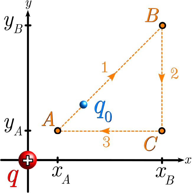
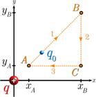
Under these previous conditions, we will calculate the work done on the test charge as it moves along the closed path, as shown in Figure 1, which is defined as follows:

Figure 1
Two-dimensional closed path traversed by the test charge.

1. The test charge starts from the initial position(x_A, y_A)and moves radially outward at an angle of 45° in relation to both axis;

2. Next, it moves parallel to the y-axis in the negative direction until it returns to the initial y-coordinate,yA;

3. Finally, it moves parallel to the x-axis in the negative direction until it returns to the initial position.

We consider the test charge moving at a constant speed, maintaining its kinetic energy throughout its motion along a simple closed two-dimensional path, specifically a triangular trajectory. This choice of path facilitates the illustration of the physical phenomenon for beginners encountering the topic for the first time. Additionally,it simplifies the calculation of the integrals required to determine the total work done, while preserving the fundamental physical concepts underlying the described phenomenon. Due to the closed trajectory is composed of three straight segments, the total amount of work can be expressed as the sum of the work contributions required to move the charge along each of the individual segments as follows:

(1) $$W_{\mathrm{Total}}=W_1+W_2+W_3.$$

Defining the position vectors of the triangular trajectory vertex A, B and C as,

(2) $$\begin{array}{cc}\hfill {\overrightarrow{r}}_A& =x_A\mathrm{}\widehat{x}+y_A\mathrm{}\widehat{y},\hfill \\ \hfill {\overrightarrow{r}}_B& =x_B\mathrm{}\widehat{x}+y_B\mathrm{}\widehat{y},\hfill \\ \hfill {\overrightarrow{r}}_C& =x_B\mathrm{}\widehat{x}+y_A\mathrm{}\widehat{y}.\hfill \end{array}$$

For the first segment of the path, the work calculation is simplified because the displacement is purely radial. Since the electrostatic force also acts along the radial direction $\widehat{r}$, the force and displacement vectors are parallel. Consequently, the dot product in the work integral $\left(\int \overrightarrow{F}\cdot \mathit{d}\overrightarrow{\ell }\right)$ reduces to a simple scalar integral $\left(\int F\mathit{d}r\right)$, and the limits of integration become the initial and final radial distances,

(3) $$\begin{array}{cc}\hfill W_1& =\underset{\mathrm{path1}}{\int }\left(k_e\frac{q{q}_0}{r^2}\widehat{r}\right)\cdot \left(dr\widehat{r}\right)=k_{e}q{q}_0\underset{r_A}{\overset{r_B}{\int }}\frac{dr}{r^2}.\hfill \end{array}$$

In other words, the amount of work will only depend on the variation in the distance between the charges from the initial to the final position. Solving the integral,

(4) $$\begin{array}{cc}\hfill W_1& =k_{e}q{q}_0{\left[-\frac{1}{r}\right]}_{r_A}^{r_B}=-k_{e}q{q}_0\left(\frac{1}{r_B}-\frac{1}{r_A}\right).\hfill \end{array}$$

This result shows that the work done to move the charge q₀ depends only on its initial and final positions. This work is the negative change in a quantity we define as the electric potential energy (U_e)of the charge q₀ due to its interaction with q. The fact that the work $\left(W=-\Delta U_e\right)$ is independent of the path taken confirms that the electrostatic force is conservative. Therefore, the work performed is entirely converted into a change in electric potential energy. The potential energy for the interaction between two point charges is thus given by $U_e=k_e\frac{q{q}_0}{r}$, which is inversely proportional to the distance r between them. Thus, the work done on the charge q₀,

(5) $$W_1=-\left[U_e\left(r_B\right)-U_e\left(r_A\right)\right]=-\left(k_e\frac{q{q}_0}{r_B}-k_e\frac{q{q}_0}{r_A}\right).$$

Next, we calculate the work done on the charge q₀ along a purely vertical path. Since work is defined by the dot product of force and displacement $\left(\overrightarrow{F}\cdot d\overrightarrow{\ell }\right)$, only the vertical component of the electric force will contribute to the work along this path. To perform the integration, we express the force in Cartesian components and set the integration limits according to the initial and final vertical positions of the trajectory.

(6) $$\begin{array}{cc}\hfill W_2& =\underset{\text{path 2}}{\int }\left(k_e\frac{q{q}_0}{\left(x_B^2+y^2\right)}\frac{\left(x_B\widehat{x}+y\mathrm{}\widehat{y}\right)}{\sqrt{x_B^2+y^2}}\right)\cdot \left(dy\mathrm{}\widehat{y}\right),\hfill \\ & =k_{e}q{q}_0\underset{y_B}{\overset{y_A}{\int }}\frac{y}{{\left(x_B^2+y^2\right)}^{\frac{3}{\text{2}}}}dy.\hfill \end{array}$$

Solving the integral,

(7) $$W_2=k_{e}q{q}_0{\left[\frac{-1}{\sqrt{x_B^2+y^2}}\right]}_{y_B}^{y_A}=-k_{e}q{q}_0\left(\frac{1}{r_C}-\frac{1}{r_B}\right).$$

Then, we can express the amount of work along this second path as,

(8) $$W_2=-\left[U_e\left(r_C\right)-U_e\left(r_B\right)\right].$$

Similarly to the previous situation, but in this case, the displacement occurs along the x-axis. We calculate the amount of work done on the charge q₀ along the third path,

(9) $$\begin{array}{cc}\hfill W_3& =\underset{\text{path 3}}{\int }\left(k_e\frac{q{q}_0}{\left(x^2+y_A^2\right)}\frac{\left(x\mathrm{}\widehat{x}+y_A\mathrm{}\widehat{y}\right)}{\sqrt{x^2+y_A^2}}\right)\cdot \left(dx\mathrm{}\widehat{x}\right),\hfill \\ & =k_{e}q{q}_0\underset{x_B}{\overset{x_A}{\int }}\frac{x}{{\left(x^2+y_A^2\right)}^{\frac{3}{\text{2}}}}dx.\hfill \end{array}$$

Solving the integral,

(10) $$W_3=k_{e}q{q}_0{\left[\frac{-1}{\sqrt{x^2+y_A^2}}\right]}_{x_B}^{x_A}=-k_{e}q{q}_0\left(\frac{1}{r_A}-\frac{1}{r_C}\right).$$

Thus, we can express the amount of work along this third path as,

(11) $$W_3=-\left[U_e\left(r_A\right)-U_e\left(r_C\right)\right].$$

In summary, using the results from (5), (8) e (11), we obtain that the total amount of work eq. (1), required to move the electric charge q₀ along a closed path at a constant speed is,

(12) $$W_{\text{Total}}=0\text{J}.$$

Therefore, the work done to move the charge from its initial to its final position is the negative of the work done to return it. This particular result shows that the net work done by the electric force over a closed path is zero. While this constitutes a specific demonstration, the null net work is the defining characteristic of a conservative force. This outcome provides compelling evidence that the electrostatic force is a conservative force, a property that can be further validated by visualizing other specific cases without making a rigorous demonstration as shown in Appendix A. The work done against a conservative force is stored as potential energy $\left(W=-\Delta U_e\right)$. This stored energy is then fully recovered as work when the charge returns to its starting point, ensuring that the total work for the round trip is zero. Mathematically, this is expressed as $\oint \overrightarrow{F}\cdot \mathit{d}\overrightarrow{\ell }=0$ for any closed trajectory.

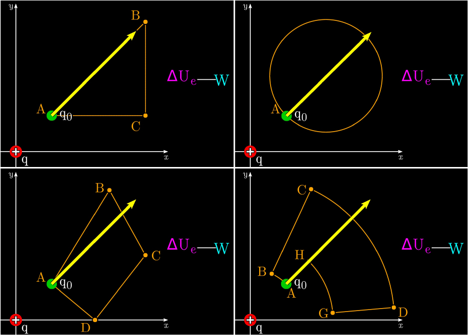
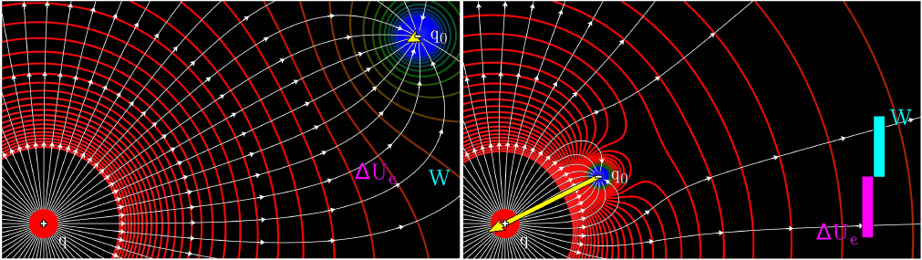
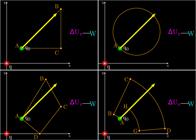
To further illustrate the conservative nature of the electrostatic force, Figure 2 presents four distinct closed paths: the triangle previously discussed, a circle, a parallelogram, and a modified polar section. In each case, a test charge moves at a constant speed and returns to its starting point. Although their algebraic descriptions are not provided here, they are slightly more elaborate yet do not complicate the understanding of the described phenomenon. We recommend the reader watch the videos by clicking here to gain a better understanding of the fact that the electric force is conservative [¹⁰]. This video tracks the work done on the charge and the corresponding change in its potential energy, visually confirming that for any closed path, both the net work done and the net change in potential energy are zero upon completion of the trajectory.

Figure 2
Four different kinds of closed trajectories traversed by the test charge.

3.Vectorial and Scalar Physical Quantities

This section explores the relationship between electric force and electric potential energy. These two concepts are fundamentally distinguished by their physical nature: electric force is a vector quantity, possessing both magnitude and direction, whereas electric potential energy is a scalar quantity, described by magnitude alone.

3.1 Electric force and electric potential energy

If we alternatively represent the variation of electric potential energy $\Delta U_e$ experienced by a point test charge q₀ between two different distances relative to a fixed point charge q using the Fundamental Theorem of Calculus, this approach provides a clear framework for analysis. It allows us to denote a definite integral that is physically associated with the cumulative contribution of infinitesimal variations in electric potential energy as the test charge is displaced. Consequently, the limits of integration correspond to the initial position r and the final position position r_f. According to the Fundamental Theorem of Calculus, this integral is equivalent to the difference in electric potential energy evaluated at the upper and lower limits,

(13) $$\underset{r_i}{\overset{r_f}{\int }}\mathit{d}{U}_e=U_e\left(r_f\right)-U_e\left(r_i\right)=\Delta U_e.$$

On the other hand, the law of conservation of energy states that the amount of work done on the electric charge to displace it is related to the negative of the variation in electric potential energy and the change in kinetic energy during this process, $W=-\Delta U_e+\Delta E_k$. However, if we consider the motion with a constant speed along the path from the initial position ${\overrightarrow{r}}_i$ to the final position ${\overrightarrow{r}}_f$, the change in kinetic energy is zero. Then, the variation of electric potential energy can be expressed as the negative of the amount of work done by the electric force ${\overrightarrow{F}}_e$ along the path taken,

(14) $$\Delta U_e=-\underset{\text{path}}{\int }{\overrightarrow{F}}_e\cdot d\overrightarrow{\ell }=-\underset{r_i}{\overset{r_f}{\int }}{F}_{\parallel }d\ell ,$$

where $F_{\parallel }$ is the component of the electric force parallel to the infinitesimal displacement $d\ell$ along the path. Because the electric force is conservative, the amount of work done is independent of the path taken and depends only on the initial and final positions between the charges, these are the integration limits. Additionally, the negative sign means that the energy required to perform the work is converted into increasing the electric potential energy of the charge. In other words, when the electric force does positive work, the potential energy decreases, and vice versa.

Additionally, by equating eq. (13) and eq. (14), it is observed that both integrals have the same defined limits, and thus their integrands are also equal and have physical units of energy. Consequently, the infinitesimal variation of the electric potential energy is expressed as,

(15) $$d{U}_e=-F_{\parallel }d\ell .$$

We can express the parallel component of the electric field along the path by isolating it from the last equation. This can be formulated in terms of the variation of electric potential energy with respect to displacement,

(16) $$F_{\parallel }=-\frac{d{U}_e}{d\ell }.$$

Therefore, the magnitude of the component of the electric force parallel to the trajectory can be described as the negative instantaneous rate of change of electric potential energy in that direction. In the particular case of the Cartesian coordinate system, with coordinate axes $\widehat{x}$, $\widehat{y}$ and $\widehat{z}$, the electric force vector can be expressed from the three-dimensional knowledge of the function representing the electric potential energy, the derivatives with respect to each Cartesian axis must be expressed as partial derivatives,

(17) $${\overrightarrow{F}}_e=-\left(\frac{\partial }{\partial x}\widehat{x}+\frac{\partial }{\partial y}\widehat{y}+\frac{\partial }{\partial z}\widehat{z}\right)U_e(x,y,z).$$

The previous result can be summarized using the notation of the differential operator nabla in Cartesian coordinates, $\nabla =\frac{\partial }{\partial x}\widehat{x}+\frac{\partial }{\partial y}\widehat{y}+\frac{\partial }{\partial z}\widehat{z}$, acting on the electric potential energy,

(18) $${\overrightarrow{F}}_e=-\nabla U_e.$$

This fundamental equation shows that the force vector, a vector quantity, points in the direction of the steepest decrease of the scalar potential energy function, which is a scalar quantity. This indicates that natural systems tend to evolve toward spatial configurations where the potential energy decreases. This principle, deriving a vector quantity from the gradient of a scalar function, is fundamental in physics. However, it is often more powerful to describe the properties of space itself, independent of any test charge placed within it. To explore its most important application in this context, we will now examine the relationship between the electric field and the electric potential.

3.2 Electric field and electric potential

The mathematical treatment connecting force and potential energy, $\overrightarrow{F}=-\nabla U_e$, reflects a fundamental physical relationship. To generalize this relation and describe the space as modified by a charge q, we define two quantities that are independent of the test charge q₀: the electric field and the electric potential. The electric field is defined as the electric force per unit of charge $\overrightarrow{E}={\overrightarrow{F}}_e/q_0$. Its physical significance is that it represents the vector property of space at a given point, quantifying the strength and direction of the force that would be exerted on any charge placed there. Analogously, the Electric Potential is defined as the Electric Potential Energy per unit charge $V=U_e/q_0$. It represents the scalar property of space at a given point, quantifying the potential energy that would be conferred to any charge placed there.

Dividing eq. (18) by q₀, we obtain the direct connection between these two essential properties of space,

(19) $$\overrightarrow{E}=-\nabla V.$$

This expression rigorously demonstrates that the electric field $\overrightarrow{E}$ at a point is the negative gradient of the electric potential V at the same point. It is important to clarify that the action of the differential operator on a scalar function, which in this particular case is $\nabla V$, represents the gradient of the electric potential. The gradient is a vector that points in the direction of the steepest ascent of a scalar function, in this case, the electric potential, and its magnitude indicates the rate of increase in that direction. Consequently, $-\nabla V$ points in the direction of the steepest descent of the electric potential. Physically, this means the field points in the direction in which the potential decreases most rapidly, solidifying the concept that both $\overrightarrow{E}$ and V describe the state of perturbation of space caused by the electric charge q. Therefore, this fundamental relationship allows one to determine the entire vector field from the spatial variation of the simpler scalar potential function.

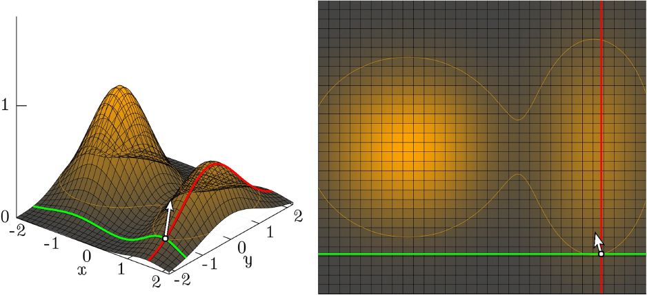
Since the gradient of a function can be a mathematically abstract concept for those encountering it for the first time, Figure 3 presents the surface plot of a simple two-dimensional function f(x,y): two Gaussian bell curves, one of which is asymmetric. The gradient vectors $\nabla f$ are shown projected onto the xy-plane, as they indicate the direction of steepest ascent in the function’s domain. To make this concept more visually intuitive on the function’s surface, we define the slope along the $\widehat{z}$-axis of the gradient vector as the norm of the partial derivatives, $\sqrt{{\left(\partial f/\partial x\right)}^2+{\left(\partial f/\partial y\right)}^2}$. Additionally, we encourage the reader to watch a short animation by clicking here to complement this discussion with a more detailed visual explanation [¹¹].

Figure 3
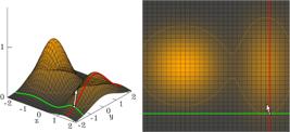
Gradient vector at a point of analysis on the surface of a two-dimensional function: perspective view (left) and top-down view (right).

3.3 Representation of the electric fieldand potential

The point charge is an idealization that treats a charge distribution as a single point of negligible size. This approximation simplifies the analysis of the resulting electric field and potential in the surrounding space. Since the electric field is a vector field, it can be visualized using a vector map. In two dimensions, this is typically represented by a grid of vectors, where each vector’s direction and magnitude correspond to the electric field at that point.

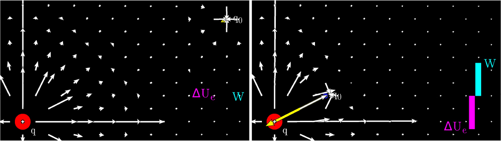
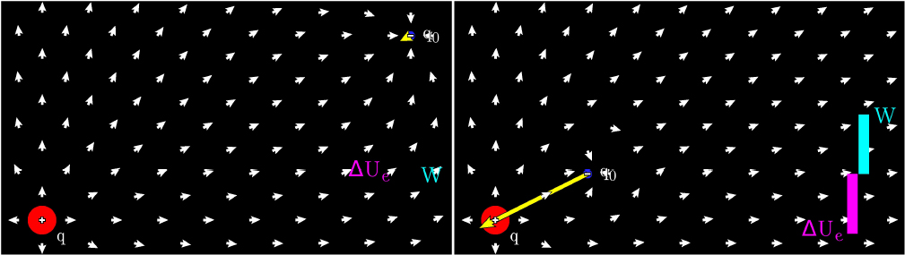
The inverse square dependence of the electric field’s magnitude on distance, $E\propto 1/r^2$, poses a significant challenge for direct vector visualization. For a point charge, this large dynamic range means that field vectors become imperceptibly small at large distances while appearing overwhelmingly large near the charge’s location Although this representation faithfully reflects the physical nature of the electric field, it can hinder effective visualization, as shown in Figure 4, where a negative point charge approaches a positive point charge with a magnitude ten times greater. Additionally, the electric force increases as the distance between the charges decreases, potentially exceeding the scale of the graph.

Figure 4
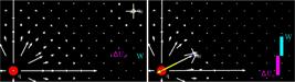
Representation of the electric field around a fixed point charge with a magnitude ten times greater than that of the test charge.

To overcome the visualization challenge posed by the field’s large dynamic range, one common approach is to represent the field’s direction only. This is achieved by normalizing each electric field vector to a constant length, effectively creating a map of unit vectors $\widehat{E}=\overrightarrow{E}/\parallel \overrightarrow{E}\parallel$. The length of these vectors is chosen for visual clarity, ensuring they do not overlap. As shown in the upper panels of Figure 5, this method effectively illustrates the directional structure of the field surrounding the charges.

Figure 5
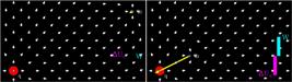
Representation of the direction of the electric field using small vectors of constant magnitude but variable direction.

A second visualization method, pioneered by Michael Faraday, represents the electric field using lines of force [¹²]. These lines provide an intuitive map of the field by encoding its properties into their geometry. By convention:

1. Lines originate on positive charges and terminate on negative charges.

2. The tangent to a line at any point gives the direction of the electric field at that point.

3. The density of the lines in a region is proportional to the field’s magnitude.

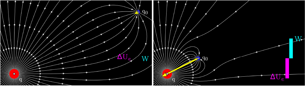
A direct consequence of the second rule is that electric field lines cannot intersect, as this would imply multiple directions for the electric field at a single location, which is physically impossible. This powerful qualitative tool is illustrated in the lower panels of Figure 6.

Figure 6
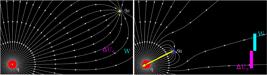
The electric field represented by field lines generated uniformly around the positive charge and end at the negative charge.

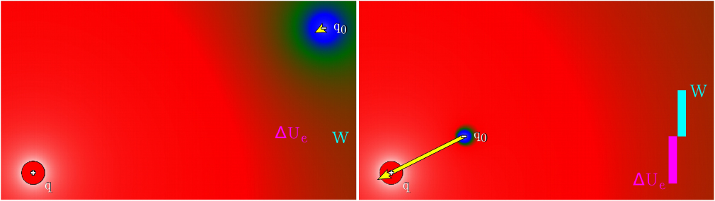
The scalar electric potential V, is often visualized using a color map, where the color at each point corresponds to the potential’s value. While this method, shown in Figure 7, accurately displays the potential across the entire space, interpreting the underlying vector field from it can be challenging. The continuous color variation can make it difficult to intuitively grasp the direction and magnitude of the field, which depends on the potential’s gradient.

Figure 7
Pictorial representation of the electric potential around electric charges.

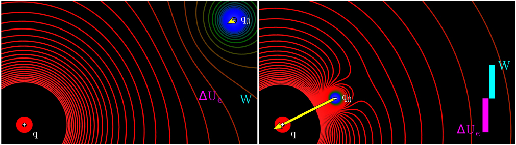
A more effective and standard method for visualizing the scalar potential is to plot its equipotential surfaces (in 3D) or equipotential lines (in 2D). These are contours that connect all points in space sharing the same constant value of electric potential, as illustrated in Figure 8. This approach simplifies the visualization from a continuous color map to a discrete set of lines, revealing the structure of the potential more clearly.

Figure 8
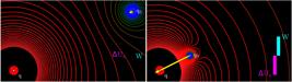
Simplified representation of the electric potential through equipotential lines in the space around electric charges.

Crucially, equipotential lines hold a fundamental relationship with the electric field: they are always perpendicular to the electric field lines. This orthogonality provides a powerful qualitative tool, as the direction of the electric field can be immediately inferred from the geometry of the equipotentials.

To synthesize this discussion, in Figure 9, we represent the electric field lines and equipotential curves in the same image, providing a comprehensive visualization of the electric field and potential distribution around charges. Electric field lines, which originate from positive charges and terminate at negative charges, illustrate the direction and relative magnitude of the electric field. The density of these lines indicates the strength of the field, with closer lines representing stronger fields. On the other hand, equipotential curves represent the positions where the electric potential has a constant value. These curves are always perpendicular to the electric field lines, highlighting the fact that no work is done by the electric field when moving a charge along an equipotential line. This combined visualization aids in understanding the spatial relationship between the electric field and potential, reinforcing key concepts such as the conservative nature of the electric force and the directional properties of field lines and potentials.

Figure 9
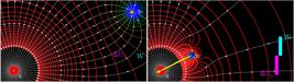
Two-dimensional representation of electric field lines and equipotential curves associated with the presence of two point charges.

3.4 Equipotential curves and field lines

The orthogonality between electric field lines and equipotential surfaces is a direct mathematical consequence of the relationship $\overrightarrow{E}=-\nabla V$. To understand this fact, let us first consider the definition of an equipotential surface: it is a locus of points in space where the scalar potential V has a constant value.

Now, imagine an infinitesimal displacement vector, $d\overrightarrow{\ell }$, that lies tangent to this equipotential surface at any given point. By definition, as we move along this path, the potential does not change. Therefore, the differential change in potential, $dV$, must be zero.

The fundamental relationship between the differential change in a scalar field and its gradient is given by $dV=\nabla V\cdot d\overrightarrow{\ell }$. This equation states that the change in potential in the direction of $d\overrightarrow{\ell }$ is the projection of the gradient vector onto that direction.

For our specific case of moving along an equipotential, we must have:

(20) $$dV=\nabla V\cdot d\overrightarrow{\ell }=0.$$

Since neither the gradient vector $\nabla V$ (which represents the maximum rate of change) nor the displacement vector $d\overrightarrow{\ell }$ are generally zero, their dot product can only be zero if the two vectors are perpendicular to each other. This proves a critical point: the gradient of the potential, $\nabla V$, is always normal (perpendicular) to the equipotential surface at every point.

Finally, since the electric field is simply the negative of the gradient $\overrightarrow{E}=-\nabla V$, it must also be normal to the equipotential surface. Consequently, the electric field lines, which trace the direction of the $\overrightarrow{E}$ vector, must intersect equipotential curves at right angles. For a dynamic visualization of this fact, the reader is directed to the supplementary animation in [¹³]. Physically, this means that no work is done by the electric field when a charge moves along an equipotential, as the electric force is always perpendicular to the displacement.

3.5 Calculation of electric field from the electric potential

To illustrate the calculation of the electric field from the electric potential in eq. (19), we will consider the two-dimensional electric potential generated by a point charge q located at the origin of the Cartesian coordinate system. Thus, at any position (x, y), the potential is expressed as,

(21) $$V(x,y)=k_e\frac{q}{\sqrt{x^2+y^2}}.$$

Whose partial derivatives with respect to the coordinate x and y are,

(22) $$\frac{\partial V}{\partial x}=-k_e\frac{qx}{{\left(x^2+y^2\right)}^{\frac{3}{\text{2}}}},\mathrm{}\frac{\partial V}{\partial y}=-k_e\frac{qy}{{\left(x^2+y^2\right)}^{\frac{3}{\text{2}}}}.$$

Based on the previous result, we will calculate the electric field $\overrightarrow{E}$ by taking the negative gradient of the electric potential. Thus, we obtain,

(23) $$\overrightarrow{E}=-\left(\frac{\partial V}{\partial x}\widehat{x}+\frac{\partial V}{\partial y}\widehat{y}\right)=-\left(-k_e\frac{q\left(x\widehat{x}+y\widehat{y}\right)}{{\left(x^2+y^2\right)}^{\frac{3}{\text{2}}}}\right).$$

To provide a clearer expression of the electric field vector and its dependence on the distance from the point (x, y) to the charge q, we factor the denominator of the expression,

(24) $$\overrightarrow{E}=k_e\frac{q}{\left(x^2+y^2\right)}\left[\frac{\left(x\widehat{x}+y\widehat{y}\right)}{\sqrt{x^2+y^2}}\right].$$

The first term corresponds to the magnitude of the electric field E at the point of analysis, while the term in brackets represents the unit vector $\widehat{r}$, which indicates the relative direction of the position of the point of analysis with respect to the electric charge. Thus, the electric field vector is expressed as,

(25) $$\overrightarrow{E}=E\widehat{r}.$$

Therefore, it is observed that the intensity of the electric field generated by a point charge decreases with the square of the distance to the point of analysis and points in the radial direction relative to the charge.

4. Algorithm to Generate Electric Field Lines

Visualizing the continuous paths of electric field lines requires a numerical algorithm that approximates these curves with a series of discrete steps. This section outlines an iterative method for generating such lines. The core principle involves starting from a set of initial points in the vicinity of a source charge and propagating a path by taking successive small steps, where the direction of each step is tangent to the local electric field vector.

4.1 Initial setup

The algorithm begins by defining the positions of two point charges, q_a and q_b, at coordinates (x_a, y_a) and (x_b, y_b), respectively. The coordinates of the positive charge, qa, are particularly important, as the electric field lines will originate from its vicinity.

4.2 Field calculation and line propagation

Next, the total electric field is expressed by its Cartesian components, E_x and E_y, at an arbitrary point of analysis (x₁, y₁). For numerical accuracy, the field generated by the two charges is formulated as follows:

(26) $$\begin{array}{cc}\hfill E_x& =k_e{q}_a\frac{\left(x_1-x_a\right)}{r_{1a}^3}+k_e{q}_b\frac{\left(x_1-x_b\right)}{r_{1b}^3},\hfill \\ \hfill E_y& =k_e{q}_a\frac{\left(y_1-y_a\right)}{r_{1a}^3}+k_e{q}_b\frac{\left(y_1-y_b\right)}{r_{1b}^3}.\hfill \end{array}$$

where the distances are $r_{1a}=\sqrt{{\left(x_1-x_a\right)}^2+{\left(y_1-y_a\right)}^2}$ and $r_{1b}=\sqrt{{\left(x_1-x_b\right)}^2+{\left(y_1-y_b\right)}^2}$. The initial points for the field lines are distributed in a circle of a small radius r around the positive charge, with their angular positions determined by:

0

(27)$$\begin{array}{cc}\hfill x_1& =x_a+r\mathrm{}\cos \left(2\pi \left(j-1\right)/N\right),\hfill \\ \hfill y_1& =y_a+r\mathrm{}\sin \left(2\pi \left(j-1\right)/N\right).\hfill \end{array}$$

Here, j is an integer counter from 1 to N, where N is the total number of lines to be plotted. This setup ensures that the initial points are evenly distributed around the charge. The direction of propagation depends on the initial sign of the E_x component. If E_x < 0 (typically for points in the first and fourth quadrants relative to the charge), the field line will propagate in the positive x-direction. Conversely, if E_x < 0 (for points in the second and third quadrants), the line will propagate in the negative x-direction.

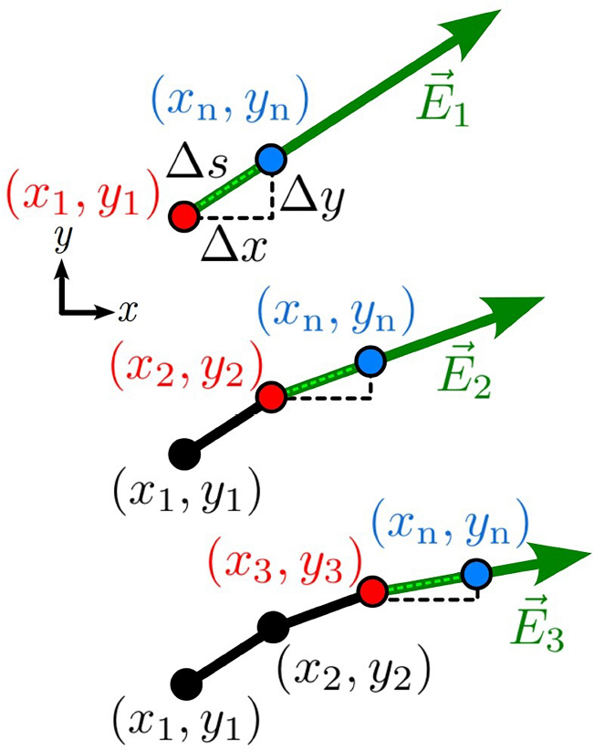
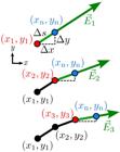
To trace a line, we iteratively find the next point (x_n, y_n) at a small distance $\Delta s$ from the current point (x₁, y₁), as shown in Figure 10. The new point must lie on the line segment tangent to the electric field at the current point, satisfying the equations:

Figure 10
Pictorial representation of the algorithm for visualizing electric field lines.

(28) $$y_{\text{n}}=y_0+\frac{E_y(x_1,y_1)}{E_x(x_1,y_1)}\left(x_{\text{n}}-x_1\right),$$

and,

(29) $${\left(\Delta s\right)}^2={\left(\Delta x\right)}^2+{\left(\Delta y\right)}^2.$$

By substituting the first relation into the second, we can solve for the x-coordinate of the next point:

(30) $$x_{\text{n}}=x_1\pm \frac{\Delta s}{\sqrt{1+{\left(E_y/E_x\right)}^2}}.$$

The choice of the sign depends on the direction of the x-component of the electric field to ensure the line propagates forward:

(31) $$\{\begin{array}{cc}\text{Use ’+’ sign}\hfill & \text{if}\mathrm{}{E}_x>0\text{(line grows to the right)}\hfill \\ \text{Use ’-’ sign}\hfill & \text{if}\mathrm{}{E}_x<0\text{(line grows to the left)}\hfill \end{array}$$

Line Termination Condition

To stop the propagation of a field line, a termination condition is imposed. The algorithm ceases to extend a line once its current point enters a small radius r around the negative charge q_b. That is, the line is truncated if $\sqrt{{\left(x_{\text{n}}-x_{\text{n-1}}\right)}^2+{\left(y_{\text{n}}-y_{\text{n-1}}\right)}^2}<r$.

Algorithm Pseudocode

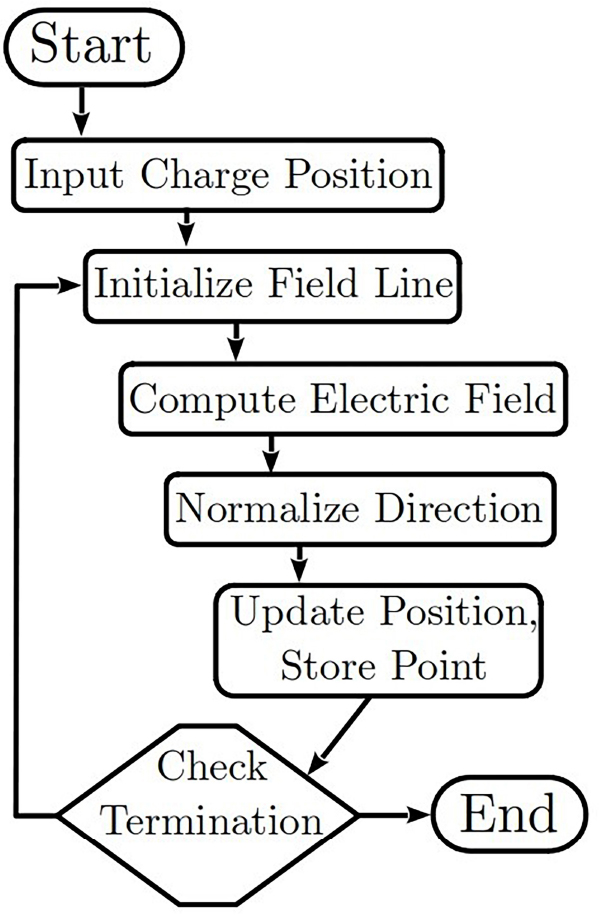
To make the algorithm’s description more accessible and less dense for beginning students, it is helpful to first build a qualitative understanding through direct interaction. Web-based applications, such as the simulations available at [¹⁴, ¹⁵], allow students to intuitively explore how electric field lines behave by simply placing charges and observing the resulting pattern. Following this initial exploration, the pseudocode block below is provided. This scheme serves as a roadmap for the computational logic behind such simulations, dividing the process into sequential and manageable steps: system setup, iterative propagation of each field line, and the termination conditions. A summary of the complete algorithm used to generate the electric field lines is presented in Figure 11.

Figure 11
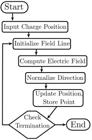
Flowchart of the algorithm for generating electric field lines, showing the iterative steps from charge input to termination.

// 1. INPUTS AND SETUP Define charge values (q_a,q_b) and positions (pos_a,pos_b). Define number of lines (N), step size (ds), and start/stop radii. // 2. MAIN LOOP (For each field line) FOR each line ’j’ from 1 to N: // a. Calculate Initial Point Calculate starting point (x,y) on a circle around pos_a. Initialize a list to store the points for this line. // b. Propagate the Line (Inner Loop) LOOP for a maximum number of steps: Add current point (x,y) to the line’s point list. // c. Calculate the Direction Calculate the electric field vector (Ex,Ey) at point (x,y). Normalize the vector to get the direction (dir_x,dir_y). // d. Take a Step Update (x,y) by moving a distance ’ds’ in the calculated direction. // e. Check Termination Condition IF the new point (x,y) is close to the negative charge q_b: BREAK LOOP END IF END LOOP END FOR // 3. OUTPUT Plot the lists of points for each of the N lines.

Zero-Field Point Calculation

Consider a configuration of two point charges: a positive charge +q_a located at the origin and a negative charge −q_b located at x = d on the x-axis. We can find a point along this axis where the net electric field is zero. Assuming q_a and q_b represent the positive magnitudes of the charges, the net field at a position x is,

(32) $$E_x=k_e\frac{q_a}{x^2}-k_e\frac{q_b}{{\left(d-x\right)}^2}.$$

Setting E_x = 0 at the null point x₀ gives:

(33) $$\frac{q_a}{x_0^{\text{2}}}=\frac{q_b}{{\left(x_0-d\right)}^2},\mathrm{}\to \left(1-\frac{q_b}{q_a}\right)x_0^{\text{2}}-2x_{0}d+d^2=0,$$

which solution is,

(34) $$x_0=\frac{2d\pm \sqrt{4d^2-4d^2\left(1-q_b/q_a\right)}}{2\left(1-q_b/q_a\right)}=\frac{d\left(1+\sqrt{q_b/q_a}\right)}{1-q_b/q_a}.$$

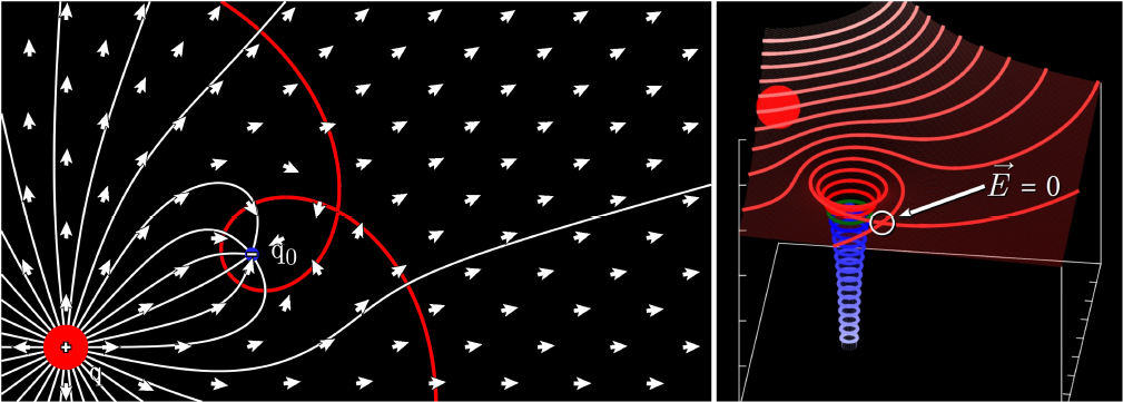
The solution to this quadratic equation gives the position x₀ of the null point. This location is a critical point in the potential landscape, specifically a saddle point, as visualized in Figure 12 and in the supplementary video [¹⁶]. At this point, the gradient of the potential is zero, which physically corresponds to a zero electric field $\overrightarrow{E}=-\nabla V=0$. The electric potential at this specific location can then be calculated by,

Figure 12
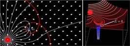
Visualization of the electric potential. The self-intersecting equipotential line (left) and the saddle point in the potential surface (right) both mark the location where the electric field is zero $\overrightarrow{E}=0$.

(35) $$V_0=k_e\frac{q_a}{x_0}-k_e\frac{q_b}{\left(x_0-d\right)}.$$

5. Considerations

Throughout this article, we have journeyed from the tangible concept of mechanical work to the abstract yet powerful ideas of fields and potentials that govern the electrostatic world. We began by demonstrating, through direct calculation, that the work done by the electric force is independent of the path taken, establishing its conservative nature. This fundamental property allowed us to define the scalar potential energy, U_e, a physical concept that simplifies problem-solving by focusing on initial and final states rather than the journey between them.

By generalizing from force and energy to their perunit-charge counterparts, we introduced the electric field, $\overrightarrow{E}$, and the electric potential, V. The core of our discussion culminated in the fundamental relationship $\overrightarrow{E}=-\nabla V$, which shows how the vector field can be derived from the gradient of the simpler scalar potential. We explored how this elegant mathematical connection manifests visually through the orthogonality of electric field lines and equipotential curves. These visualization techniques are not mere illustrations; they are conceptual tools that provide deep insight into the structure and behavior of electric fields.

This exploration was designed to be a gentle introduction, showing that even the most abstract concepts in physics are built upon a foundation of logical, sequential steps. The principles discussed here: conservative forces, potentials, and the gradient relationship, are not confined to electrostatics; they are recurring themes throughout physics, appearing in gravitation, fluid dynamics, and beyond. It is our hope that this didactic approach has illuminated these foundational concepts, providing the reader with the confidence and curiosity to continue exploring the elegant mathematical structure of our physical universe.

Acknowledgments

My deepest gratitude goes to the students of the Chemistry Education program, whose thoughtful curiosity and insightful questions about the physical meaning of electrostatic concepts have continuously inspired me. Their engagement has encouraged me to seek clearer and more meaningful ways to explain principles that are foundational to their future careers. I would also like to express my sincere appreciation to my college Sandro, whose valuable time, constructive comments, and academic guidance have greatly contributed to the refinement of this work.

Supplementary Material

The following supplementary material is available online:

Appendix A

- Work done by the electrostatic force on a closed path.

Data Availability

All data generated or analyzed during this study are included in this published article and its supplementary information files.

References

• ^[1] D.J. Griffiths, Introduction to Electrodynamics (Cambridge University Press, 2017), 4 ed.
• ^[2] D. Halliday, R. Resnick and J. Walker, Fundamentals of Physics (Wiley, 2018), 11 ed.
• ^[3] H.D. Young and R.A. Freedman, University Physics with Modern Physics (Pearson, San Francisco, 2016), v. 3, 14 ed.
• ^[4] E.M. Purcell and D.J. Morin, Electricity and Magnetism (Cambridge University Press, Cambridge, 2013), 3 ed.
• ^[5] D.P. Maloney, T.L. O’Kuma, C.J. Hieggelke and A. Van Heuvelen, Am. J. Phys. 69, S12 (2001).
• ^[6] R. Chabay and B. Sherwood, Am. J. Phys. 74, 329 (2006).
• ^[7] E. Bagno and U. Efron, Phys. Rev. ST Phys. Educ. Res. 4, 010101 (2008).
• ^[8] E. Campos, G. Zavala, K. Zuza and J. Guisasola, Phys. Rev. Phys. Educ. Res. 16, 010135 (2020).
• ^[9] M. Newman, Computational Physics (CreateSpace Independent Publishing Platform, Scotts Valley, 2013), 2 ed.
• ^[10] D. Velasco, Work of the Electric Force in Closed Trajectories, available in: https://youtu.be/XZBA5c97ylw?si=0CoqTTS2BbIXBaJw
  » https://youtu.be/XZBA5c97ylw?si=0CoqTTS2BbIXBaJw
• ^[11] D. Velasco, Gradient of a Scalar Function, available in: https://youtu.be/-lwTn6j6Kz4
  » https://youtu.be/-lwTn6j6Kz4
• ^[12] M. Faraday, Phil. Trans. R. Soc. Lond. 128, 125 (1838).
• ^[13] D. Velasco, Electric Potential Energy and Work done - Two point charges, available in: https://youtu.be/ff4xXpcmB-Q
  » https://youtu.be/ff4xXpcmB-Q
• ^[14] ITHACA COLLEGE, DEPARTMENT OF PHYSICS AND ASTRONOMY, available in: https://icphysweb.z13.web.core.windows.net/simulation.html
  » https://icphysweb.z13.web.core.windows.net/simulation.html
• ^[15] JAVALAB SCIENCE SIMULATIONS, available in: https://javalab.org/en/electric_field_line_en/
  » https://javalab.org/en/electric_field_line_en/
• ^[16] D. Velasco, Equipotential Curve and Nule Electric Field, available in: https://youtu.be/yiqsHtPNxS8
  » https://youtu.be/yiqsHtPNxS8

Edited by

• Editor-in-Chief:
  Marcello Ferreira https://orcid.org/0000-0003-4945-3169

Publication Dates

• Publication in this collection
  12 Jan 2026
• Date of issue
  2025

History

• Received
  29 July 2025
• Reviewed
  26 Nov 2025
• Accepted
  27 Nov 2025