Simulation of diffraction patterns of annular apertures

Abstract

In this paper, Fraunhofer diffraction patterns generated by square and circular annular apertures are studied. The annular region is defined as the difference between two concentric areas of equal geometry: an outer fixed aperture and an inner closed obstacle, whose size is varied by a scaling parameter $h$. This parameter modifies the geometry of the aperture and, consequently, the shape and energy distribution in the diffraction pattern. Exact equations for intensity and analytical expressions for the fraction of energy contained in the region of maximum intensity are derived. For visualization and numerical analysis, codes are implemented in Maple 25, and a graphical user interface is designed in Python 3.13 that allows the evolution of diffraction patterns to be observed through animation as $h$ varies. The study developed may be useful in optical applications, particularly in imaging systems.

Keywords:
Fraunhofer diffraction; annular aperture; Maple simulation; Python interface; diffraction patterns

1. Introduction

Diffraction is a characteristic effect of wave phenomena [¹]; it occurs when a portion of a wavefront is intercepted by obstacles or openings [²]. As a result of this interaction, multiple segments of the wavefront are generated which, when propagating beyond the obstacle, interfere with each other, producing a characteristic energy distribution known as a diffraction pattern that acts as a fingerprint of the object [³], providing information about its geometry. This property explains the importance and wide applicability of the phenomenon in various scientific disciplines. Using diffraction, the structure of crystals, molecules, hormones, nucleic acids, enzymes, proteins, and viruses has been determined [⁴].

In acoustic engineering, this phenomenon is particularly important when barriers are used to create an acoustic shadow behind them. The acoustic shadow effect is commonly applied in outdoor environments to reduce noise from roads or railroads [⁵]. In optics, diffraction effects are of great significance in the detailed understanding of devices that contain lenses, diaphragms, slits, mirrors, and other elements. Even if all aberrations in a lens system were eliminated, the final sharpness of the image would still be limited by diffraction [⁶].

Historically, the study of diffraction at apertures has been classified into two main categories: Fresnel diffraction and Fraunhofer diffraction [⁷, ⁸]. The distinction between the two lies in the curvature of the incident and diffracted wavefronts. In this work, we focus specifically on Fraunhofer diffraction, where both the incident and diffracted wavefronts can be approximated as planar because they are considered in the far-field limit [⁹, ¹⁰].

In particular, we address the diffraction of a plane wave incident on square and circular apertures, both of which are widely documented in the literature [³, ⁸, ¹¹, ¹²]. The main motivation is to visualize, through simulation, how the intensity distribution of the diffracted wave evolves when the degree of openness of such apertures is modulated. To this end, a concentric obstacle with the same geometry as the aperture is introduced. In this way, the space between the aperture and the obstacle defines an annular region whose degree of aperture is controlled by a geometric scale parameter $h$ that varies between $0$ and $1$, where $h=0$ represents a completely clear aperture and $h=1$ a completely obstructed one.

As a result of integrating the Fraunhofer diffraction integral over the annular region, exact expressions are obtained for the field and intensity of the diffracted waves as a function of $h$. When evaluated at $h=0$, the intensity expressions reduce to the particular cases of the classical diffraction patterns of square and circular apertures. Once the intensity is determined, the energy distribution reaching an observation screen is calculated, and analytical expressions are derived for the fraction of energy contained around the region of maximum intensity. Thus, the parameter $h$ allows controlling the fraction of energy transmitted through the aperture and, consequently, observing how the diffraction pattern changes.

The equations obtained for the intensity, although exact, involve a non-trivial mathematical analysis that requires numerical methods, such as the calculation of optimal values. Likewise, the visualization of diffraction patterns requires specialized graphical tools, and the evaluation of analytical expressions for the energy fraction must be performed using numerical integration. For these reasons, we used Maple 25 as the main simulation tool. This software allows for user-friendly symbolic and numerical computation, as its built-in functions eliminate the need to develop structured numerical algorithms, as would be necessary with other computational tools [¹³]. Its use is based on commands that execute symbolic and numerical calculations according to the specified operation, reducing computational complexity to a few lines of code [¹⁴]. In addition, it provides high-resolution graphics that offer a deeper perspective on the phenomenon under study. However, Maple presents a limitation in terms of accessibility and reproducibility due to its commercial nature, since its use requires the acquisition of a license [¹⁵].

As a freely accessible educational alternative, the simulation is implemented in Python 3.13, a language that, thanks to its accessibility and widespread adoption, has become an effective tool for simulating physical phenomena [¹⁶]. An interactive graphical user interface has been designed, allowing the user to select, using radio buttons, the type of pattern to be observed (square or circular) and the desired graphical perspective (3D or profile), as well as a slider to dynamically visualize the evolution of the diffraction pattern as $h$ varies, taking advantage of Python’s capabilities to facilitate the understanding of physical phenomena through interactive visualization [¹⁷]. Although the code used for the interface includes extensive computational logic, both the code and the interface are provided through an open-access link, ensuring their availability to the academic community and their direct implementation in the classroom.

The exact equations obtained for the intensity and the analytical expressions for calculating the energy fraction complement the theoretical study of diffraction in square and circular apertures. In particular, as Hecht and Zajac [⁶] point out, the calculation of the energy fraction is a topic of interest but is highly complex. This calculation is rarely reported in textbooks, the most common case being that of the circular aperture without an obstacle [¹¹]. These results may be of particular interest in optics, especially in applications related to the resolution and design of imaging systems [¹², ¹⁸]. From a pedagogical perspective, the two computational implementations presented constitute teaching tools that can be directly integrated into the classroom, providing students with a detailed visualization of the phenomenon and revealing how, beyond the mathematical complexity of physical modeling, the results highlight the beauty and depth of the behavior of the diffraction phenomenon in nature.

2. Theory

2.1. Scalar wave diffraction

Diffraction is a characteristic effect of wave phenomena. It occurs when a portion of the wavefront is obstructed by an obstacle or aperture. That is, consider a scalar wave $\Psi (\text{r},t)$ propagating freely in the half-space $z<0$ with velocity $v$. The wave, along its path, interacts with an obstacle that has a small opening. The obstacle constitutes a portion of the closed surface $\partial \Omega$ that bounds a volume $\Omega$. In the half-space $z>0$ (the interior of $\Omega$), the field satisfies the wave equation:

(1) $${\nabla }^2\Psi (\text{r},t)=\frac{1}{v^2}{\partial }_t^2\Psi (\text{r},t),$$

with prescribed values on the boundary $\partial \Omega$. According to the method of separation of variables, a solution of the form

(2) $$\Psi (\text{r},t)=\psi \left(\text{r}\right)T\left(t\right)$$

can be assumed. By substituting this expression into equation (1), we obtain:

(3) $$\left({\nabla }^2+k^2\right)\psi \left(\text{r}\right)=0,\left({\partial }_t^2+{\omega }^2\right)T\left(t\right)=0,$$

with $\omega$ the separation constant and $k={\omega }^2/v^2$ the wave number.

For a causally propagating wave (i.e., propagating forward in time), $T\left(t\right)\sim e^{-i\omega t}$. As for the solution $\psi \left(\text{r}\right)$, which corresponds to a solution of the interior problem in $\Omega$ specified by the Helmholtz equation [¹⁹], it is given by:

(4) $$\psi \left(\text{r}\right)={\oint }_{\partial \Omega }\left[\psi \left({\text{r}}^{\prime }\right)\frac{\partial G(\text{r},{\text{r}}^{\prime })}{\partial n^{\prime }}-G(\text{r},{\text{r}}^{\prime })\frac{\partial \psi \left({\text{r}}^{\prime }\right)}{\partial n^{\prime }}\right]\mathit{d}{a}^{\prime },$$

where ${\partial }_{n^{\prime }}$ denotes the differentiation along the normal to $\partial \Omega$ and $G(\text{r},{\text{r}}^{\prime })$ is the Green’s function associated with the problem:

(5) $$\left({\nabla }^2+k^2\right)G(\text{r},{\text{r}}^{\prime })=-\delta \left(\text{r}-{\text{r}}^{\prime }\right)\forall \text{r}\in \Omega ,{\text{r}}^{\prime }\in \partial \Omega .$$

Next, suppose that the boundary $\partial \Omega$ is composed of two rigid surfaces. The first, $S_1$, corresponds to the diffracting surface – the obstacle with an opening $𝒜$ – located in the plane $z=0$, while $S_2$ extends along the edge of a sector of the half-space $z>0$. When the wave strikes the aperture in $S_1$, the field at any point inside $\Omega$ can be considered as the superposition of the field diffracted by $S_1$ and the field reflected by $S_2$. However, if we assume that $S_2$ is sufficiently far from $S_1$, the contribution from reflection vanishes (radiation condition¹) [²⁰]:

(6) $${\psi |}_{S_2}\sim \frac{e^{ikr}}{r}.$$

Thus, from equation (4) one has:

(7) $$\psi \left(\text{r}\right)={\int }_{S_1}\left[\psi \left({\text{r}}^{\prime }\right)\frac{\partial G(\text{r},{\text{r}}^{\prime })}{\partial n^{\prime }}-G(\text{r},{\text{r}}^{\prime })\frac{\partial \psi \left({\text{r}}^{\prime }\right)}{\partial n^{\prime }}\right]\mathit{d}{a}^{\prime },$$

where r represents the observation point and ${\text{r}}^{\prime }$ the source point at the aperture. This expression is known in the literature as the Helmholtz–Kirchhoff integral [¹¹].

To solve equation (7), it is necessary to specify either Dirichlet or Neumann boundary conditions on $S_1$, but not both simultaneously. In the case of Dirichlet boundary conditions, one has:

(8) $${\psi |}_{𝒜}={\psi }_0\text{and}{\psi |}_{S_1\ne 𝒜}=0.$$

Here, the Green’s function $G(\text{r},{\text{r}}^{\prime })$ must cancel out the term in the integral of equation (7) involving ${\partial }_{n^{\prime }}\psi$, which implies the condition:

(9) $${G_D(\text{r},{\text{r}}^{\prime })|}_{S_1}=0.$$

On the other hand, under Neumann conditions, we have:

(10) $${{\partial }_{n^{\prime }}\psi |}_{𝒜}={\partial }_{n^{\prime }}{\psi }_0\text{and}{{\partial }_{n^{\prime }}\psi |}_{S_1\ne 𝒜}=0.$$

In this case, the Green’s function $G(\text{r},{\text{r}}^{\prime })$ must cancel the term containing $\psi \left({\text{r}}^{\prime }\right)$, leading to:

(11) $${{\partial }_{n^{\prime }}{G}_N(\text{r},{\text{r}}^{\prime })|}_{S_1}=0.$$

A special case in which the Green’s function satisfies the conditions stated in equations (9) and (11) is when $S_1$ is an infinite flat screen located at $z=0$ [²⁰]. In this configuration, the Green’s function is given by:

(12) $$G_{D,N}(\text{r},{\text{r}}^{\prime })=\frac{1}{4\pi }\frac{e^{ik\left|\text{r}-{\text{r}}^{\prime }\right|}}{\left|\text{r}-{\text{r}}^{\prime }\right|}\mp \frac{1}{4\pi }\frac{e^{ik\left|\text{r}-{\text{r}}^{\prime \prime }\right|}}{\left|\text{r}-{\text{r}}^{\prime \prime }\right|}.$$

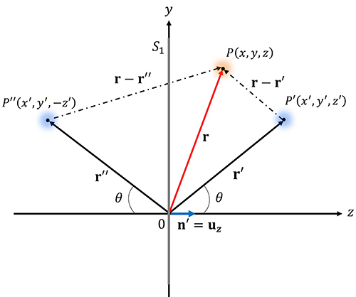
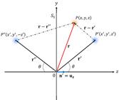
This equation is constructed using the method of images, considering the geometric arrangement illustrated in Fig. 1. The subscripts $D$ and $N$ are associated with the $-$ and $+$ signs, respectively. In this formulation, ${\text{r}}^{\prime \prime }$ represents the position of the image source with unit magnitude. The point $P$ corresponds to the location where the scalar field is evaluated by superposition of the contributions from the source and its image. Since the screen is at $z=0$, the normal derivative reduces to the derivative with respect to $z$. If we evaluate at $z=0$ in terms of cartesian coordinates, we obtain:

(13)$$\left|\text{r}-{\text{r}}^{\prime }\right|=\left|\text{r}-{\text{r}}^{\prime \prime }\right|=\sqrt{{\left(x-x^{\prime }\right)}^2+{\left(y-y^{\prime }\right)}^2+{\left(z^{\prime }\right)}^2}.$$

Figure 1
Point source and its image.

It follows that $G_D$ cancels out, and its derivative with respect to $z$ turns out to be:

(14) $${\frac{\partial G_D(\text{r},{\text{r}}^{\prime })}{\partial z}|}_{z=0}=\frac{1}{2\pi }\left(\frac{1}{\left|\text{r}-{\text{r}}^{\prime }\right|}-ik\right)\frac{z^{\prime }}{{\left|\text{r}-{\text{r}}^{\prime }\right|}^2}{e}^{ik\left|\text{r}-{\text{r}}^{\prime }\right|}.$$

On the other hand, in the Neumann case, we have that ${\partial }_z{G}_N$ cancels out, and the Green’s function takes the form:

(15) $${G_N(\text{r},{\text{r}}^{\prime })|}_{z=0}=\frac{1}{2\pi }\frac{e^{ik\left|\text{r}-{\text{r}}^{\prime }\right|}}{\left|\text{r}-{\text{r}}^{\prime }\right|}.$$

Finally, by substituting equation (14) into equation (7), the diffracted scalar field under Dirichlet conditions is expressed as:

(16) $${\psi }_D\left(\text{r}\right)=\frac{1}{2\pi }{\int }_{𝒜}\psi \left({\text{r}}^{\prime }\right)\left(\frac{1}{\left|\text{r}-{\text{r}}^{\prime }\right|}-ik\right)\frac{z}{{\left|\text{r}-{\text{r}}^{\prime }\right|}^2}{e}^{ik\left|\text{r}-{\text{r}}^{\prime }\right|}\mathit{d}{a}^{\prime }.$$

Similarly, for Neumann conditions, by substituting equation (15) into equation (7), one obtains:

(17) $${\psi }_N\left(\text{r}\right)=-\frac{1}{2\pi }{\int }_{𝒜}{\partial }_{z^{\prime }}{\psi }_0\frac{e^{ik\left|\text{r}-{\text{r}}^{\prime }\right|}}{\left|\text{r}-{\text{r}}^{\prime }\right|}d{a}^{\prime }.$$

These expressions are known in the literature as the Rayleigh–Sommerfeld integrals [¹⁹]. Note that in equation (16), we have $z^{\prime }\leftrightarrow z$. The coordinate $z^{\prime }$ corresponds to the position of the source, adjacent to the aperture plane, used in the construction of the Green’s function. When substituted into equation (7), this coordinate corresponds to the $z$-component of the point at which the scalar field is evaluated.

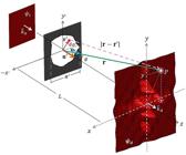
Fig. 2 illustrates the diffraction geometry described by equations (16) and (17), with the origins of the vectors r and ${\text{r}}^{\prime }$ located at the center of the aperture. In particular, it shows a plane wave of wavelength $\lambda$ that is normally incident on an aperture of characteristic size $a^{\prime }$. The diffracted wave changes its shape as it propagates into the half-space $z>0$ and acquires a more defined structure as it moves away from the aperture. At a sufficiently large axial distance $L$, the wavefronts reaching the observation point $P$ are almost flat. This far-field region corresponds to the Fraunhofer regime, where the distance $L$ satisfies the condition:

$$L\gg \frac{a^{\prime 2}}{\lambda }.$$

Figure 2
Diffracted scalar wave.

Next, the behavior of the diffracted wave in the far-field limit is analyzed.

2.2. Fraunhofer diffraction

This work considers the diffraction of a plane wave by an aperture, as illustrated in Fig. 2. The diffracted wave is evaluated on a screen, referred to as the observation plane, located in the far field at a distance $z=L$ from the center of the aperture.

Mathematically, the incident plane wave is modeled as:

(18) $${\psi }_i(\text{r},t)={\psi }_0\left(\text{r}\right)e^{i\left(kz-\omega t\right)},$$

where ${\psi }_0$ represents the amplitude of the wave, $k=2\pi /\lambda$ is the wavenumber associated with the wavelength $\lambda$, and $\omega$ is the angular frequency. In the plane over $𝒜$ ($z=0$), the spatial part of the incident wave reduces to:

(19) $${{\psi }_i\left(\text{r}\right)|}_{z=0}={\psi }_0.$$

This indicates that the field intensity distribution over $𝒜$ is uniform.

The diffraction of a plane wave, or any type of wave, occurs when the characteristic size of the aperture is comparable to or smaller than the wavelength, that is, when $k{r}^{\prime }\ll 1$[¹]. Under these conditions, the intensity distribution on the diffracted wavefront contains information about the geometry of the aperture, which becomes clearly observable in the far field, when the wavefront reaching the screen is approximately flat. Since $r$ defines all observation points on the screen and $r^{\prime }$ all source points in the aperture, in the far-field regime it holds that $r\gg r^{\prime }$[⁶]. This relationship between the magnitudes of the vectors r and ${\text{r}}^{\prime }$ allows us to simplify the differences $\left|\text{r}-{\text{r}}^{\prime }\right|$ in the algebraic terms of the integrals (16) and (17). However, the phase term $k\left|\text{r}-{\text{r}}^{\prime }\right|$ determines the curvature of the wavefront and, therefore, must be approximated with greater care in the far-field limit. The objective of this approximation is to identify the phase term corresponding to a plane wave arriving at the screen. To perform this approximation, the binomial expansion [²¹] is used as a mathematical tool:

(20) $${\left(1-x\right)}^{\alpha }=1-\alpha x+\frac{\alpha \left(\alpha -1\right)}{2}{x}^2+\dots ;\alpha \in ℝ,\left|x\right|<1.$$

We apply this expansion to the phase term $k\left|\text{r}-{\text{r}}^{\prime }\right|$ of equation (16). Rewriting the phase:

$$k\left|\text{r}-{\text{r}}^{\prime }\right|=k{\left(r^{\prime 2}+r^2-2\text{r}\cdot {\text{r}}^{\prime }\right)}^{1/2}$$ $$=k{\left(r^{\prime 2}+r^2-2\text{r}\cdot {\text{r}}^{\prime }\right)}^{1/2}$$

Expanding to second order, we obtain:

(21) $$\begin{array}{l}k\left|\text{r}-{\text{r}}^{\prime }\right|=kr-{\displaystyle \frac{kr}{2}}\left({\displaystyle \frac{2{\text{r}}^{\prime }\cdot {\text{u}}_r}{r}}-{\displaystyle \frac{r^{\prime 2}}{r^2}}\right)\\ +{\displaystyle \frac{kr}{8}}{\left({\displaystyle \frac{2{\text{r}}^{\prime }\cdot {\text{u}}_r}{r}}-{\displaystyle \frac{r^{\prime 2}}{r^2}}\right)}^2+\dots \\ =kr-k{\text{r}}^{\prime }\cdot {\text{u}}_r+{\displaystyle \frac{kr}{2}}\left[r^{\prime 2}+{\left({\text{r}}^{\prime }\cdot {\text{u}}_r\right)}^2\right]+\dots \end{array}$$

From this equation, we will consider only the first two terms, which are those that define Fraunhofer diffraction [¹⁹]. The higher-order terms are considered negligible compared to unity and tend to vanish as $r$ tends to infinity.

Substituting the above result, equation (21), together with equation (19), into equation (16), we obtain:

(22) $$\psi \left(\text{r}\right)=\frac{{\psi }_0}{2\pi }{\int }_{𝒜}\left(\frac{1}{\left|\text{r}-{\text{r}}^{\prime }\right|}-ik\right)\frac{z{e}^{ikr}}{{\left|\text{r}-{\text{r}}^{\prime }\right|}^2}{e}^{-ik{\text{r}}^{\prime }\cdot {\text{u}}_r}\mathit{d}{a}^{\prime }.$$

Since $r\gg r^{\prime }$, the term $1/\left|\text{r}-{\text{r}}^{\prime }\right|\to 0$ and ${\left|\text{r}-{\text{r}}^{\prime }\right|}^2\sim r^2$. Consequently, equation (22) reduces to:

(23) $$\begin{array}{l}\psi \left(\text{r}\right)=-{\displaystyle \frac{ik{\psi }_0}{2\pi }}{\displaystyle {\int }_{𝒜}}{\displaystyle \frac{z{e}^{ikr}}{r^2}}{e}^{-ik{\text{r}}^{\prime }\cdot {\text{u}}_r}\mathit{d}{a}^{\prime }\\ =-{\displaystyle \frac{ik{\psi }_{0}z{e}^{ikr}}{2\pi r^2}}{\displaystyle {\int }_{𝒜}}{e}^{-ik{\text{r}}^{\prime }\cdot {\text{u}}_r}\mathit{d}{a}^{\prime }.\end{array}$$

From Fig. 2, it is seen that the square of the modulus of the vector r is given by:

$$r^2=z^2\left(1+\frac{x^2+y^2}{z^2}\right)=z^2\left(1+{\tan }^2\theta \right),$$

where $\theta$ is the angle between the vector r and the $z$-axis. For large values of $z$, the angle $\theta$ is small, which implies that ${\tan }^2\theta \ll 1$. Consequently, when the observation plane is at a sufficiently large distance $z=L$, we have $r\sim L$.

Considering these approximations, and expanding the scalar product ${\text{u}}_r\cdot {\text{r}}^{\prime }\simeq \left(x{x}^{\prime }+y{y}^{\prime }\right)/L$, equation (23) simplifies as:

(24) $$\psi (x,y)\simeq -\frac{ik{\psi }_0{e}^{ikL}}{2\pi L}{\int }_{𝒜}{e}^{-\frac{ik}{L}\left(x{x}^{\prime }+y{y}^{\prime }\right)}\mathit{d}{a}^{\prime }.$$

This equation is the Fraunhofer diffraction integral [⁸, ¹¹, ¹²], which represents the Fourier transform of the aperture function and is used in the study of diffraction by small apertures in the far-field regime. The term $e^{ikL}$ indicates that the fields in the plane $z=L$ behave like plane waves. In this domain, the aperture acts as a continuous distribution of secondary sources whose waves interfere constructively and destructively in the observation plane.

3. Square and Circular Annular Aperture

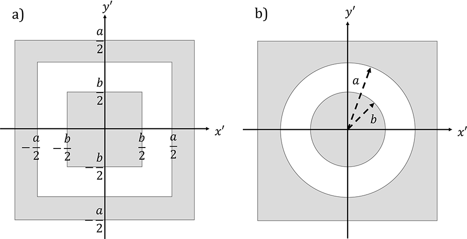
Fig. 3 shows the apertures considered in this study. The first corresponds to a square annular aperture, defined between sides $a$ and $b$, while the second represents a circular annular aperture, bounded between radii $a$ and $b$.

Figure 3
Annular apertures: a) square, b) circular.

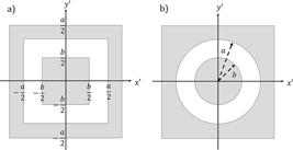
The square annular region, Fig. 3a, is mathematically expressed as:

$${𝒜}_s=\left\{(x^{\prime },y^{\prime })\right|-{\displaystyle \frac{a}{2}}\le x^{\prime }\le {\displaystyle \frac{a}{2}},-{\displaystyle \frac{a}{2}}\le y^{\prime }\le {\displaystyle \frac{a}{2}}\}\setminus$$ $$\left\{(x^{\prime },y^{\prime })\right|-{\displaystyle \frac{b}{2}}\le x^{\prime }\le {\displaystyle \frac{b}{2}},-{\displaystyle \frac{b}{2}}\le y^{\prime }\le {\displaystyle \frac{b}{2}}\}.$$

Evaluating the Fraunhofer integral, equation (24), we obtain:

(25) $$\begin{array}{l}\psi (x,y)=-{\displaystyle \frac{ik{\psi }_0{e}^{ikL}}{2\pi L}}[{\displaystyle {\int }_{-\frac{a}{2}}^{\frac{a}{2}}}{\displaystyle {\int }_{-\frac{a}{2}}^{\frac{a}{2}}}{e}^{-\frac{ik}{L}\left(x{x}^{\prime }+y{y}^{\prime }\right)}d{x}^{\prime }d{y}^{\prime }\\ -{\displaystyle {\int }_{-\frac{b}{2}}^{\frac{b}{2}}}{\displaystyle {\int }_{-\frac{b}{2}}^{\frac{b}{2}}}{e}^{-\frac{ik}{L}\left(x{x}^{\prime }+y{y}^{\prime }\right)}d{x}^{\prime }d{y}^{\prime }].\end{array}$$

Integrating equation (25), results in:

(26) $$\begin{array}{l}\psi (x,y)=-{\displaystyle \frac{ik{\psi }_0{e}^{ikL}}{2\pi L}}\cdot {\displaystyle \frac{4L^2}{xy{k}^2}}[\sin \left({\displaystyle \frac{kxa}{2L}}\right)\sin \left({\displaystyle \frac{kya}{2L}}\right)\\ -\sin \left({\displaystyle \frac{kxb}{2L}}\right)\sin \left({\displaystyle \frac{kyb}{2L}}\right)].\end{array}$$

Here, we have used the identity $2i\sin \left(\theta \right)=\left(e^{i\theta }-e^{-i\theta }\right)$. For simplicity, the dimensionless coordinates $\overline{x}=\left(kxa/2L\right)$ and $\overline{y}=\left(kya/2L\right)$ are defined, turning equation (26) into:

(27) $$\begin{array}{l}\psi (\overline{x},\overline{y})=-{\displaystyle \frac{ik{\psi }_0{e}^{ikL}}{2\pi L}}\cdot {\displaystyle \frac{\left(a^2-b^2\right)a^2}{\left(a^2-b^2\right)\overline{x}\overline{y}}}[\sin \left(\overline{x}\right)\sin \left(\overline{y}\right)\\ -\sin \left({\displaystyle \frac{b}{a}}\overline{x}\right)\sin \left({\displaystyle \frac{b}{a}}\overline{y}\right)].\end{array}$$

Finally, the parameter $h$ is introduced as a scaling factor defining the ratio between the inner and outer dimensions of the aperture. In particular, it is defined as $b=ha$, with $0\le h\le 1$, where $h=0$ represents a completely clear aperture, while $h=1$ indicates a completely closed aperture. With this definition, equation (27) is rewritten as:

(28) $$\begin{array}{l}\psi (\overline{x},\overline{y})={\displaystyle \frac{ik{A}_s{\psi }_0{e}^{ikL}}{2\pi L\left(1-h^2\right)\overline{x}\overline{y}}}\\ \cdot \left[\sin \left(\overline{x}\right)\sin \left(\overline{y}\right)-\sin \left(h\overline{x}\right)\sin \left(h\overline{y}\right)\right],\end{array}$$

with $A_s=\left(a^2-b^2\right)$ being the area of the aperture. The equation gives the scalar field diffracted by a square annular aperture in terms of the dimensionless coordinates $\overline{x}$ and $\overline{y}$.

In the case of the circular annular aperture, depicted in Fig. 3b, the symmetry of the problem suggests the use of polar coordinates. Therefore, the circular annular region is mathematically expressed as:

$${𝒜}_c=\{(r^{\prime },{\theta }^{\prime })\mid b\le r^{\prime }\le a,0\le {\theta }^{\prime }<2\pi \}.$$

Thus, considering the aperture plane, the Cartesian coordinates are expressed as $x^{\prime }=r^{\prime }\cos {\theta }^{\prime }$ and $y^{\prime }=r^{\prime }\sin {\theta }^{\prime }$, while in the observation plane we define $x=\rho \cos \Theta$ and $y=\rho \sin \Theta$. With these changes, equation (24) is rewritten as:

(29) $$\psi (r,\Theta )=-\frac{ik{\psi }_0{e}^{ikL}}{2\pi L}{\int }_b^a{\int }_0^{2\pi }{e}^{-\frac{ik\rho r^{\prime }}{L}\cos \left({\theta }^{\prime }-\Theta \right)}{r}^{\prime }\mathit{d}{r}^{\prime }\mathit{d}{\theta }^{\prime },$$

where the trigonometric identity corresponding to the difference of angles in the cosine function² has been applied, and the area element has been rewritten in its polar form, $d{a}^{\prime }=r^{\prime }d{r}^{\prime }d{\theta }^{\prime }$. Due to the complete axial symmetry of the system, the solution must be independent of $\Theta$. This allows us to consider the particular case $\Theta =0$ without loss of generality. Therefore, the portion of the double integral associated with the variable ${\theta }^{\prime }$ is evaluated as:

(30) $${\int }_0^{2\pi }{e}^{-\frac{ik\rho r^{\prime }}{L}\cos {\theta }^{\prime }}\mathit{d}{\theta }^{\prime }=2\pi J_0\left(\frac{k\rho r^{\prime }}{L}\right),$$

where $J_0$ is the zeroth-order Bessel function. Applying this result to equation (29), we obtain:

(31) $$\psi \left(\rho \right)=-\frac{ik{\psi }_0{e}^{ikL}}{L}{\int }_b^a{J}_0\left(\frac{k\rho r^{\prime }}{L}\right)r^{\prime }\mathit{d}{r}^{\prime }.$$

Applying the change of variable $u=k\rho r^{\prime }/L$, and using the recurrence relation of Bessel functions, $D_u\left[u^m{J}_m\left(u\right)\right]=u^m{J}_{m-1}\left(u\right)$ for $m=1$, the final result of the integral is:

(32) $$\begin{array}{l}\psi \left(\rho \right)=-{\displaystyle \frac{ik{\psi }_0{e}^{ikL}}{L}}\left[{\displaystyle \frac{La}{k\rho }}{J}_1\left({\displaystyle \frac{k\rho a}{L}}\right)-{\displaystyle \frac{Lb}{k\rho }}{J}_1\left({\displaystyle \frac{k\rho b}{L}}\right)\right]\\ =-{\displaystyle \frac{ik{\psi }_0{e}^{ikL}}{2\pi L}}\cdot {\displaystyle \frac{2\pi \left(a^2-b^2\right)}{\left(a^2-b^2\right)}}[{\displaystyle \frac{La}{k\rho }}{J}_1\left({\displaystyle \frac{k\rho a}{L}}\right)\\ -{\displaystyle \frac{Lb}{k\rho }}{J}_1\left({\displaystyle \frac{k\rho b}{L}}\right)].\end{array}$$

In this equation, analogous to equation (26), we define the dimensionless radial coordinate $\overline{\rho }=ka\rho /L$ and the parameter $h$ as a scaling factor that determines the ratio between the inner and outer radii of the aperture, i.e., $b=ha$, yielding:

(33) $$\psi \left(\overline{\rho }\right)=\frac{ik{\psi }_0{A}_c{e}^{ikL}}{2\pi L}\cdot \frac{2}{\left(1-h^2\right)\overline{\rho }}\left[J_1\left(\overline{\rho }\right)-h{J}_1\left(h\overline{\rho }\right)\right],$$

with $A_c=\pi \left(a^2-b^2\right)$ being the area of the aperture. The equation gives the scalar field diffracted by a circular annular aperture in terms of the dimensionless coordinate $\overline{\rho }$.

Equations (28) and (33) describe the spatial distribution of the diffracted wave. Since these functions are generally complex, their evaluation requires considering the physical field, i.e., the part of the wave that is observable or detectable. In practice, it is more convenient to analyze the field intensity rather than the field itself. For example, in optics, the high frequencies of electromagnetic waves make direct field measurement impractical; therefore, we work with irradiance, measured in units of power per unit area ($W/m^2$), which is proportional to the real part of the square of the electric field modulus.

Similarly, for scalar waves in general, the quantity of interest is the intensity $I$, defined in terms of the square of the modulus of the scalar field:

(34) $$I\propto {\Vert \psi \Vert }^2.$$

Substituting equation (28), we obtain the expression for the relative intensity in the square annular aperture:

(35) $$\frac{I(\overline{x},\overline{y})}{I_0}=\frac{1}{{\left(1-h^2\right)}^2}{\left[\frac{\sin \left(\overline{x}\right)\sin \left(\overline{y}\right)}{\overline{x}\overline{y}}-\frac{\sin \left(h\overline{x}\right)\sin \left(h\overline{y}\right)}{\overline{x}\overline{y}}\right]}^2,$$

and from equation (33), the expression for the circular annular aperture:

(36) $$\frac{I\left(\overline{\rho }\right)}{I_0}=\frac{4}{{\left(1-h^2\right)}^2}{\left[\frac{J_1\left(\overline{\rho }\right)}{\overline{\rho }}-\frac{h{J}_1\left(h\overline{\rho }\right)}{\overline{\rho }}\right]}^2.$$

Here, $I_0={\left(ikA{\psi }_0{e}^{ikL}/2\pi L\right)}^2$ represents a normalization constant proportional to the total scalar wave energy measured at a reference point $P_0$ in the observation plane. The ratio $I/I_0$ characterizes the relative intensity $I_r$, which constitutes the Fraunhofer diffraction pattern. The parameter $h$ modulates the shape of the pattern, allowing us to analyze the effect that the geometry of the aperture has on the distribution of the diffracted energy.

When evaluating at $h=0$, equations (35) and (36) reduce to the classical cases of diffraction by square and circular apertures, respectively:

$$I_r(\overline{x},\overline{y})={\left[\frac{\sin \left(\overline{x}\right)\sin \left(\overline{y}\right)}{\overline{x}\overline{y}}\right]}^2,$$ $$I_r\left(\overline{\rho }\right)={\left[\frac{2J_1\left(\overline{\rho }\right)}{\overline{\rho }}\right]}^2.$$

In this limit, the parameter $h$ no longer influences the intensity distribution, and the resulting pattern corresponds to that of a simple aperture.

It is important to note that the harmonic structures of equations (35) and (36) generate regions in the plane where the energy is maximized and minimized until it cancels out completely. Given this behavior, it is relevant to study the fraction of incident energy $F$ contained in a region $D$, bounded by optimal points.

This energy fraction is calculated by the following expression [¹²]:

(37) $$F=\frac{\underset{D}{\iint }{I}_r\mathit{d}\overline{a}}{\underset{-\infty }{\overset{+\infty }{\int }}\underset{-\infty }{\overset{+\infty }{\int }}{I}_r\mathit{d}\overline{a}},$$

where $I_r$ represents the relative intensity and $d\overline{a}$ is the area element in dimensionless coordinates.

For the case of the square annular aperture, the integration of equation (35) over the entire plane is considered. The corresponding integral is:

$${\displaystyle {\int }_{-\infty }^{+\infty }}{\displaystyle {\int }_{-\infty }^{+\infty }}{\displaystyle \frac{1}{{\left(1-h^2\right)}^2}}$$ $$\cdot {\left[{\displaystyle \frac{\sin \left(\overline{x}\right)\sin \left(\overline{y}\right)}{\overline{x}\overline{y}}}-{\displaystyle \frac{\sin \left(h\overline{x}\right)\sin \left(h\overline{y}\right)}{\overline{x}\overline{y}}}\right]}^{2}d\overline{x}d\overline{y}.$$

Expanding the binomial and taking advantage of the symmetry of the relative intensity with respect to $\overline{x}$ and $\overline{y}$, $I_r(x,y)=I_r(-x,-y)$, the expression is rewritten as:

$$\begin{array}{l}{\displaystyle \frac{4}{{\left(1-h^2\right)}^2}}[{\displaystyle {\int }_0^{\infty }}{\displaystyle {\int }_0^{\infty }}{\displaystyle \frac{{\sin }^2\left(\overline{x}\right){\sin }^2\left(\overline{y}\right)}{{\overline{x}}^2{\overline{y}}^2}}\\ +{\displaystyle \frac{{\sin }^2\left(h\overline{x}\right){\sin }^2\left(h\overline{y}\right)}{{\overline{x}}^2{\overline{y}}^2}}\\ -{\displaystyle \frac{2\sin \left(\overline{x}\right)\sin \left(\overline{y}\right)\sin \left(h\overline{x}\right)\sin \left(h\overline{y}\right)}{{\overline{x}}^2{\overline{y}}^2}}].\end{array}$$

The factored form of the integrands allows the integrals to be solved separately, reducing them to the product of integrals of the type [²²]:

$${\int }_0^{\infty }\frac{\sin \left(au\right)\sin \left(bu\right)}{u^2}\mathit{d}u=\frac{b\pi }{2},\text{with}0<b\le a.$$

Applying this identity to the integral expressions above, we obtain:

(38) $$\frac{4}{{\left(1-h^2\right)}^2}\left[\frac{{\pi }^2}{4}+\frac{{\pi }^2{h}^2}{4}-\frac{{\pi }^2{h}^2}{2}\right]=\frac{{\pi }^2}{1-h^2}.$$

Therefore, if $D$ is a rectangular region of the observation plane defined by the domain $R=[{\overline{x}}_1,{\overline{x}}_2]\times [{\overline{y}}_1,{\overline{y}}_2]$, then by substituting equation (38) in the denominator into equation (37), the energy fraction is expressed as:

(39) $$\begin{array}{l}F(\overline{x},\overline{y})={\displaystyle \frac{1-h^2}{{\pi }^2}}{\displaystyle {\int }_{{\overline{x}}_1}^{{\overline{x}}_2}}{\displaystyle {\int }_{{\overline{y}}_1}^{{\overline{y}}_2}}{I}_r(\overline{x},\overline{y})\mathit{d}\overline{x}\mathit{d}\overline{y}\\ ={\displaystyle \frac{1}{{\pi }^2\left(1-h^2\right)}}\\ \cdot {\displaystyle {\int }_{{\overline{x}}_1}^{{\overline{x}}_2}}{\displaystyle {\int }_{{\overline{y}}_1}^{{\overline{y}}_2}}{\left[{\displaystyle \frac{\sin \left(\overline{x}\right)\sin \left(\overline{y}\right)-\sin \left(h\overline{x}\right)\sin \left(h\overline{y}\right)}{\overline{x}\overline{y}}}\right]}^2\\ \cdot d\overline{x}d\overline{y}.\end{array}$$

On the other hand, for the circular annular aperture, the integration of equation (36) in polar coordinates is considered. The integral over the entire domain is:

$${\int }_0^{\infty }{\int }_0^{2\pi }\left[\frac{4}{{\left(1-h^2\right)}^2}{\left(\frac{J_1\left(\overline{\rho }\right)}{\overline{\rho }}-\frac{h{J}_1\left(h\overline{\rho }\right)}{\overline{\rho }}\right)}^2\right]\overline{\rho }\mathit{d}\overline{\theta }\mathit{d}\overline{\rho }.$$

Integrating with respect to the variable $\overline{\theta }$ and expanding the binomial, we obtain:

$$\frac{8\pi }{{\left(1-h^2\right)}^2}\left[{\int }_0^{\infty }\frac{J_1^2\left(\overline{\rho }\right)}{\overline{\rho }}+\frac{h^2{J}_1^2\left(h\overline{\rho }\right)}{\overline{\rho }}-\frac{2h{J}_1\left(\overline{\rho }\right)J_1\left(h\overline{\rho }\right)}{\overline{\rho }}d\overline{\rho }\right].$$

Each of these integrals is of the type [²³]:

$${\int }_0^{\infty }\frac{J_1\left(au\right)J_1\left(bu\right)}{u}\mathit{d}u=\frac{b}{2a},b\le a.$$

Applying this identity, we obtain the following result:

(40) $$\frac{8\pi }{{\left(1-h^2\right)}^2}\left[\frac{1}{2}+\frac{h^2}{2}-h^2\right]=\frac{4\pi }{1-h^2}.$$

Finally, if $D$ is a circular region of radius $\overline{\rho }$ in the observation plane, the contained energy fraction is obtained by substituting the result of equation (40) into the denominator of equation (37). The expression is:

(41) $$\begin{array}{l}F\left(\overline{\rho }\right)={\displaystyle \frac{1-h^2}{4\pi }}{\displaystyle {\int }_0^{\overline{\rho }}}2\pi I_r\left(\overline{\rho }\right)\overline{\rho }\mathit{d}\overline{\rho }\\ ={\displaystyle \frac{2}{1-h^2}}{\displaystyle {\int }_0^{\overline{\rho }}}{\left[{\displaystyle \frac{J_1\left(\overline{\rho }\right)-h{J}_1\left(h\overline{\rho }\right)}{\overline{\rho }}}\right]}^2\mathit{d}\overline{\rho }.\end{array}$$

Since the exact analytical solutions of equations (3) and (41) are not trivial, we resort to numerical implementation in Maple 25 and Python 3.13 to evaluate the fraction of contained energy in different regions of interest and analyze its behavior as a function of $h$.

4. Diffraction Patterns

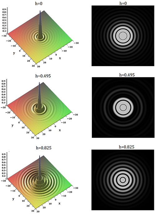
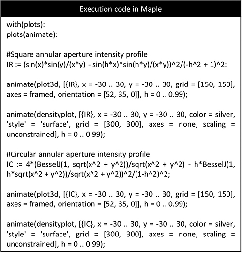
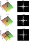
The Maple 25 software was used, as the first option, to simulate the diffraction patterns of the apertures under study. Fig. 4 and Fig. 5 present the surface plots and diffraction patterns corresponding to the square annular and circular annular apertures, respectively, for $h$ values of $0$, $0.495$, and $0.825$. The code used in the Maple worksheet to generate these plots is shown in Fig. 6.

Figure 4
Relative intensity and diffraction patterns of the square annular aperture.

Figure 5
Relative intensity and diffraction patterns of the circular annular aperture.

Figure 6
Maple code for simulation of diffraction patterns.

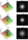
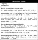
For the visualization and animation of the plots, the packages with(plots) and with(animate) were used. The variables IR and IC represent equations (35) and (36), respectively. The execution of the commands plot3d and densityplot, together with animate, allows observing the evolution of the intensity distribution and diffraction pattern as the parameter $h$ varies in the interval $0\le h<0.99$.

In the simulation, we set $h=0.99$ as the upper bound instead of $h=1$. This was done in order to ensure the proper execution of the code by avoiding potential errors that may arise due to the singularity of the $1/\left(1-h^2\right)$ term in equations (35) and (36).

These figures show that the relative intensity decays rapidly with distance, presenting a central peak of maximum intensity normalized to unity. The results obtained for $h=0$ are consistent with the diffraction patterns of square and circular apertures reported in the literature [³, ⁸, ¹¹, ¹²].

The parameter $h$ significantly modifies the geometry of the diffraction pattern. As $h$ increases in the square annular aperture, the pattern evolves into a more complex configuration with the appearance of square dark edges around the central maximum. In the circular annular aperture, on the other hand, the increase in $h$ mainly alters the distribution of the concentric rings, making them more pronounced.

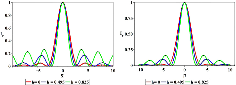
Fig. 7 shows the intensity cross-sectional profiles, highlighting the first three intensity maxima and minima. The corresponding optimal values are shown in Tables 1 and 2.

Figure 7
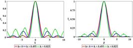
Relative intensity $I_r$ for different values of the scale factor $h$: a) Square annular aperture, b) Circular annular aperture.

Table 1
Intensity maxima and minima of the square annular aperture.

$h$	$I_{\max }^1$	$X_{\max }^1$	$I_{\min }^1$	$X_{\min }^1$	$I_{\max }^2$	$X_{\max }^2$	$I_{\min }^2$	$X_{\min }^2$	$I_{\max }^3$	$X_{\max }^3$	$I_{\min }^3$	$X_{\min }^3$
0.000	1.000	0.000	0.000	$\pm 3.142$	0.047	$\pm 4.493$	0.000	$\pm 6.283$	0.016	$\pm 7.725$	0.000	$\pm 9.425$
0.495	1.000	0.000	0.000	$\pm 2.643$	0.170	$\pm 4.261$	0.000	$\pm 6.296$	0.051	$\pm 7.863$	0.000	$\pm 9.931$
0.825	1.000	0.000	0.000	$\pm 2.219$	0.261	$\pm 3.712$	0.000	$\pm 5.369$	0.224	$\pm 7.009$	0.000	$\pm 8.717$

• The notations $I_{\max }^n$, $I_{\min }^n$, $X_{\max }^n$, and $X_{\min }^n$ represent the position of the optimal values corresponding to the $n$-th maximum or minimum of relative intensity measured from the center. For $n=1$, the central maximum is identified, followed by the first minimum, until the sequence of local maxima and minima of the diffraction pattern is complete.

Table 2
Intensity maxima and minima of the circular annular aperture.

$h$	$I_{\max }^1$	${\rho }_{\max }^1$	$I_{\min }^1$	${\rho }_{\min }^1$	$I_{\max }^2$	${\rho }_{\max }^2$	$I_{\min }^2$	${\rho }_{\min }^2$	$I_{\max }^3$	${\rho }_{\max }^3$	$I_{\min }^3$	${\rho }_{\min }^3$
0.000	1.000	0.000	0.000	3.832	0.017	5.136	0.000	7.016	0.004	8.417	0.000	10.173
0.495	1.000	0.000	0.000	3.153	0.095	4.831	0.000	7.201	0.012	8.679	0.000	10.961
0.825	1.000	0.000	0.000	2.631	0.155	4.180	0.000	6.040	0.077	7.652	0.000	9.468

• The notations $I_{\max }^n$, $I_{\min }^n$, ${\rho }_{\max }^n$, and ${\rho }_{\min }^n$ indicate the locations of the optimal values corresponding to the $n$-th relative intensity value measured from the center. For $n=1$, the maximum corresponds to the center of the bright disk, and the minimum to the first dark ring surrounding it, followed by the sequence of bright and dark rings that form the diffraction pattern.

It is observed that, with increasing $h$, the primary minima shift toward the center, reducing the width of the main peak. In addition, the secondary maxima intensify and also shift their positions toward the center.

From the primary minima, the fraction of total incident energy contained in the central maximum peak is calculated using equations (3) and (41). Table 3 presents the width of the central peak and the fraction of incident energy contained in it.

Table 3
Fraction of incident energy in the central maximum of annular apertures for different values of $h$.

Parameter	Square		Circular
$h$	$\Delta x_{\min }^1$	$F\left(\Delta x_{\min }^1\right)$	$\Delta x_{\min }^1$	$F\left(\Delta x_{\min }^1\right)$
0.000	6.283	82%	7.663	84%
0.495	5.286	47%	6.306	48%
0.825	4.437	14%	5.263	15%

• The notations $\Delta X_{\min }^1$ indicate the width of the bright square region for the square aperture and the diameter of the bright disk for the circular aperture, while $F\left(\Delta X_{\min }^1\right)$ represents the fraction of energy contained within those regions.

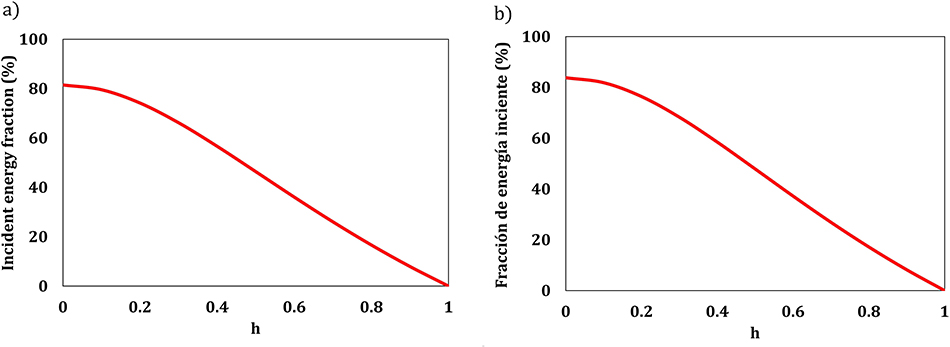
In the region bounded by the first primary minima, most of the incident energy is concentrated. This energy fraction reaches its maximum value when the aperture is completely clear. The geometry of the aperture plays a fundamental role in the redistribution of the diffracted energy; in particular, the fraction of energy contained in the central region is greater for the circular aperture than for the square one.

As our analysis demonstrates, the presence of an obstacle modifies the geometry of the aperture and, consequently, the energy distribution in the diffraction pattern. As the effective area of the aperture is reduced, the width of the central peak decreases, leading to a reduction in the fraction of energy confined to this region.

In the case of the square aperture, the decrease in energy concentration at the central maximum is compensated by an increase in the intensity of the local maxima. For the circular aperture, the same effect manifests as an increase in the intensity of the concentric rings adjacent to the central disk. The plots in Fig. 8 show the loss of energy concentration at the central maximum as the value of the parameter $h$ increases. When the reduction in the aperture area is more pronounced, the energy is more evenly distributed among the local maxima.

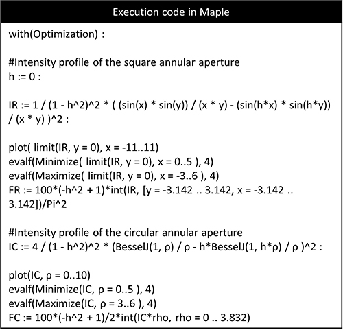
Fig. 9 presents the code used in the Maple worksheet to obtain the tabulated values. These results come from the graphical and numerical analysis of the density profile. The package with(optimization) provides tools for the direct computation of the optimal points. The commands Maximize and Minimize allow the determination of the intensity maxima and minima together with their coordinates.

Figure 8
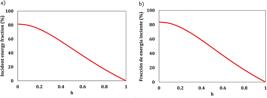
Fraction of energy contained in the central maximum as a function of the parameter $h$, for the annular apertures: (a) square and (b) circular.

Figure 9
Maple code for calculating the energy fraction in the central maximum.

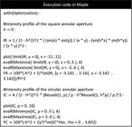
By combining these commands with evalf, the user can select the number of significant figures with which the result is to be displayed. Since the calculation of optimal values requires the specification of an interval, it is conveniently chosen based on the visualization of the graph generated with the plot command.

Notice that, for the intensity in the square aperture, the limit of IR as $y\to 0$ is used as the analysis variable, which converts IR into its one-dimensional form. Finally, the variables FR and FC are used to calculate the fraction of energy contained in the central peak by integrating the intensity in the region bounded by the first minima, according to equations (3) and (41).

5. Simulation in Python: Graphical User Interface

As noted in the previous section, Maple allows good results to be obtained in the simulation of diffraction patterns with few lines of code. However, the commercial and proprietary nature of the software limits the reproducibility of the simulation and its numerical analysis by the academic community. This motivated the development of an open-access alternative implemented in Python.

This section presents the design of a graphical user interface (GUI) in Python. Through these environments, users interact with a computer or software application using visual elements such as icons, menus, and buttons, rather than typing commands into a text-based interface [²⁴]. The result of this interaction is to display abstract and complex ideas in mathematics and physics in pictorial or graphical forms, such as those developed in various educational works [²⁵, ²⁶, ²⁷]. These interfaces are particularly suitable for the university level because of their ease of use and immediacy in displaying results.

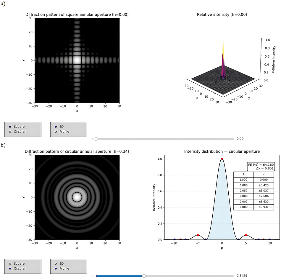
Fig. 10 shows the interface developed in Python 3.13. The diffraction patterns are displayed in the upper left corner, while the relative intensity distribution graphs are shown in the upper right corner. The lower part of the interface contains the interactive controls: in the lower left corner, there are two sets of radio buttons, and in the lower center, there is a slider to control the parameter $h$.

Figure 10
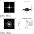
Graphical user interface in Python 3.13. (a) View for a square aperture with $h=0$, showing the diffraction pattern and 3D intensity distribution. (b) View for a circular aperture with $h=0.34$, showing the diffraction pattern and intensity profile with a table of optimal values.

The first set of radio buttons allows the user to select the type of pattern to observe: square aperture or circular aperture. The second set allows the user to choose the type of graphical perspective for the intensity distribution: three-dimensional visualization in space (depending on the selected aperture type) or density profile. This latter option highlights the point of maximum intensity, the first two local maxima, the first three local minima, and the integration region around the maximum intensity zone considered for the calculation of the energy fraction along the central peak. The profile graph is accompanied by a table with the identified optimal values and a box showing the width of the central peak and the energy fraction contained within it.

The slider continuously modulates the parameter $h$ from its initial value $h=0$ (unobstructed aperture) to values close to complete obstruction. As the control is moved, the interface displays an animated representation of how the diffraction pattern evolves, the change in relative intensity, the shift in local maxima and minima, the variation in the width of the central peak, and the redistribution of energy within it. In this way, the interface presents all the results considered in this study in an integrated and interactive manner.

The integration of interactive components, the color contrast gradient in the diffraction patterns, the numerical optimization and integration calculations, and the handling of special functions such as Bessel functions require the implementation of specialized Python library packages and a considerable number of lines of code. To ensure the automatic reproducibility of all results, an open-access link is provided with the interface in .py format for direct execution from any computer with Python installed, as well as the code in .txt format for readers interested in reproducing the simulation or adapting the logic to other software environments of their choice.

6. Conclusions

In this study, Fraunhofer diffraction patterns generated by square and circular annular apertures were simulated. The annular aperture was defined as the open space between an aperture of fixed size and an inner concentric obstacle of the same geometry, whose area is varied by a scaling parameter $h$. This parameter modifies the geometry of the aperture and, consequently, the shape and energy distribution in the diffraction pattern.

Using Maple 25 and Python 3.13 software, the evolution of the relative intensity distribution and the diffraction pattern was visualized with the increase of the parameter $h$, providing a detailed and highly informative perception of the diffraction phenomenon. It was observed that, regardless of the value of $h$, all diffraction patterns of the annular apertures studied exhibit a central intensity maximum. Taking advantage of the versatility of both platforms for performing numerical calculations, the width of the central maximum and the fraction of incident energy contained in this region were determined.

The results revealed that both the width and energy concentration of the central maximum decrease as the aperture area is reduced. This loss of energy concentration is compensated by an increase in the intensity of the secondary maxima and other peaks in the pattern. The control exerted by $h$ over the diffraction pattern may have useful applications, for example, in optics and imaging systems.

The implementation in Maple 25 and Python 3.13 presents results that are consistent with each other and with those reported in the literature for unobstructed apertures. In this sense, the choice of one program or another depends on factors such as institutional accessibility, computational ease, and user familiarity with each platform. Maple offers advantages in terms of implementation simplicity due to its built-in functions, while Python ensures accessibility and reproducibility because of its open-source nature. From a pedagogical perspective, the implemented codes and the interactive graphical interface developed in Python constitute valuable tools for courses on waves or optics, particularly in online teaching modalities that lack a physical laboratory or in institutions with financial limitations for acquiring experimental equipment. The incorporation of interactive digital tools enriches the educational process by capturing students’ attention and facilitating the understanding of complex physical phenomena through dynamic visualization.

Data Availability

The Python 3.13 graphical interface developed for this study is openly available at: https://doi.org/10.5281/zenodo.17401425 If any difficulty arises in accessing the file, it may be requested directly from the corresponding author.

Referências

• ^[1] J.M. Alvarado Reyes, A. Santos Aguilar and C.M.S. Reimer López, Rev. Mex. Fis. E 18, 50 (2021).
• ^[2] O. Helene, Í.S. Fernandes and T.G.S. Martins, Rev. Bras. Ens. Fis. 45, e20220281 (2023).
• ^[3] E. Hecht, Optics (Pearson Education, London, 2017), 5 ed.
• ^[4] M. Martínez-Ripoll and P. Román-Polo, An. Quím. 108, 225 (2012).
• ^[5] J. Piechowicz, Acta Phys. Pol. A 119, 1040 (2011).
• ^[6] E. Hecht and A. Zajac, Óptica (Addison-Wesley Iberoamericana, Wilmington, 1986).
• ^[7] F.F. Medina, Rev. Mex. Fis. 31, 311 (1984).
• ^[8] J.W. Goodman, Introduction to Fourier Optics (Macmillan Learning, New York, 2017), 4 ed.
• ^[9] D.M. Reis, E.M. Santos and A.V. Andrade-Neto, Rev. Bras. Ens. Fis. 37, 2312 (2015).
• ^[10] F.S. Crawford Jr., Ondas (Editorial Reverté, Barcelona, 1994), v. 3.
• ^[11] M. Born and E. Wolf, Principles of Optics (Cambridge University Press, Cambridge, 1997), 7 ed.
• ^[12] A. Ghatak, Optics (McGraw-Hill, New York, 2010).
• ^[13] E. Alvarado-Anell, M. Sosa and M. Moreles, Rev. Mex. Fis. E 51, 102 (2005).
• ^[14] G. Ortigoza Capetillo, Rev. Mex. Fis. E 53, 56 (2007).
• ^[15] G. Ortigoza and R.I. Ponce de la Cruz Herrera, Rev. Mex. Fis. E 20, 020209 (2023).
• ^[16] E.I.B. Rodrigues, Rev. Bras. Ens. Fís. 47, e222 (2025).
• ^[17] S.R. Oliveira, Rev. Bras. Ens. Fís. 46, e20240060 (2024).
• ^[18] J.E. Harvey and C. Ftaclas, Appl. Opt. 34, 6337 (1995).
• ^[19] J.D. Jackson, Electrodinámica Clásica (Wiley, Madrid, 1980), 3 ed.
• ^[20] M.L. Calvo Padilla, Óptica Avanzada (Ariel, Barcelona, 2002).
• ^[21] J. Stewart, Cálculo de una Variable (Cengage Learning, Ciudad de México, 2008), 6 ed.
• ^[22] I.S. Gradshteyn and I.M. Ryzhik, Table of Integrals, Series, and Products (Elsevier, New York, 2007), 7 ed.
• ^[23] G.N. Watson, A Treatise on the Theory of Bessel Functions (Cambridge University Press, Cambridge, 1966), 2 ed.
• ^[24] M.Y. Tufail and S. Gul, Rev. Mex. Fis. E 22, 010208 (2025).
• ^[25] F. Arriaga, J.P. Staneck, F. Lanzini and O. Fornaro, Anales AFA 30, 77 (2018).
• ^[26] D.H. Penalver-Vidal, D.L. Romero-Antequera and F.S. Granados-Agustín, Rev. Mex. Fis. E 59, 18 (2013).
• ^[27] A. Razzak and Z. Uddin, Rev. Mex. Fis. E 20, 010208 (2023).

• 1
  This assumption corresponds to Sommerfeld’s radiation condition, which physically excludes any incoming or reflected waves from infinity. Sommerfeld formulated the radiation condition to ensure the uniqueness of the solution to the Helmholtz equation in the exterior domain.
• 2
  $\cos \left(\alpha -\beta \right)=\cos \alpha \cos \beta +\sin \alpha \sin \beta$

Edited by

• Editor-in-Chief:
  Marcello Ferreirahttps://orcid.org/0000-0003-4945-3169

Publication Dates

• Publication in this collection
  09 Jan 2026
• Date of issue
  2025

History

• Received
  01 Aug 2025
• Reviewed
  22 Oct 2025
• Accepted
  20 Nov 2025