Is it really necessary to use complex methods for silting estimation in reservoirs?

É realmente necessário usar métodos complexos para estimar o assoreamento em reservatórios?

ABSTRACT

The study aimed to evaluate whether primary hydrosedimentometric monitoring data would be sufficient to estimate the total siltation of the Pimental Reservoir (Belo Monte HPP) or whether more complex methods would be required. Three mass balance approaches were applied: the sedimentometric method, the simplified Sediment model, and three-dimensional hydrodynamic and sediment transport modeling (Delft3D). The three-dimensional model was calibrated and the silting was evaluated for a period were observed data was available. Subsequently, a future scenario (2018–2039) was simulated based on extrapolations of existing flood hydrographs and operational data. The results showed similar average siltation rates between the sedimentometric method (1.37 hm³/year) and the 3D modeling (1.31–1.48 hm³/year), while the Sediment model overestimated siltation rates (2.29 hm³/year) because it did not represent the outflow through the diversion channel. When evaluating sedimentation rates over decades, an increase in rates was observed in the second decade for all methods. It was observed that less complex methods can provide representative estimates for siltation management, provided there is adequate monitoring, especially in the diversion channel, and monitoring during flood peaks.

Keywords:
Reservoir; Three-dimensional modelling; Mass balance; Silting rate

RESUMO

O estudo teve como objetivo avaliar se dados primários de monitoramento hidrossedimentométrico seriam suficientes para estimar o assoreamento total do reservatório de Pimental (UHE Belo Monte) ou se seriam necessários métodos mais complexos. Foram aplicadas três abordagens de balanço de massa: método sedimentométrico, modelo simplificado Sediment e modelagem hidrodinâmica e de transporte de sedimentos tridimensional (Delft3D). Foi realizada a calibração do modelo tridimensional e avaliada a sedimentação no período com dados observados. Posteriormente, foi avaliado um cenário futuro (2018–2039) com base em hidrogramas de cheia e dados operativos. Os resultados mostraram taxas médias de assoreamento semelhantes entre o método sedimentométrico (1,37 hm³/ano) e a modelagem 3D (1,31–1,48 hm³/ano), enquanto o modelo Sediment superestimou (2,29 hm³/ano) por não representar a saída pelo canal de derivação. Avaliando as taxas de sedimentação por décadas, observou-se aumento nas taxas na segunda década simulada em todos os métodos. Observou-se que métodos menos complexos podem fornecer estimativas representativas para a gestão do assoreamento, desde que haja monitoramento adequado, especialmente no canal de derivação, e monitoramento em picos de cheia.

Palavras-chave:
Reservatório; Modelagem tridimensional; Balanço de massa; Taxa de assoreamento

INTRODUCTION

Damming a river to create a reservoir reduces water velocities, and reducing sediment transport capacity, which favors sediment deposition and, therefore, reservoir silting. This, in turn, is a natural process that, over time, can reduce water storage capacity (Hilgert et al., 2024) and affect its intended uses (Endalew & Mulu, 2022). Therefore, understanding and estimating siltation are essential for water resources management. In the electricity sector, silting can directly impact water availability for hydropower electricity generation, reducing production and system reliability. Thus, studies on sedimentation rates and silted quantities are essential for system planning and operation.

In previous studies reservoir siltation has been carried out using different approaches, either through traditional bathymetry monitoring and comparison with previous measurements (Khasanov, 2025; Hilgert et al., 2024; Endalew & Mulu, 2022), sediment balances (Lemma et al., 2024; Jansson & Erlingsson, 2000), remote sensing (Yao et al., 2023; Lopes & Araújo, 2019; Collischonn & Clarke, 2016), numerical modeling or simplified models (Rabelo et al., 2025; Reisenbüchler et al., 2020; Costa et al., 2018) or a combination of these methods (Luz et al., 2025a).

Regarding bathymetric surveys, which represents the direct method of measuring siltation, Collischonn & Clarke (2016) argue that the cost of the survey depends on the location and access, reservoir volume, and level at the time of measurement. Furthermore, when comparing bathymetries, there are always doubts about the consistency of the older data, given the technologies previously adopted (Collischonn & Clarke, 2016).

In general, to calculate the estimated siltation, measurements are necessary. Brazil's river monitoring network evolved during the 20th century, primarily focused on the implementation of stations specifically designed to support studies on hydraulic developments for hydropower generation (Agência Nacional de Águas e Saneamento Básico, 2009). However, considering 2021 data from the National Water and Sanitation Agency (ANA) of the 2,024 active river measuring stations in Brazil, only 463 of them (22.9%) monitor suspended sediments (solid discharge) (Agência Nacional de Águas e Saneamento Básico, 2021). This relationship points to a historical weakness in solid discharge monitoring in Brazil, which limits, for example, analyses of siltation in hydroelectric plant reservoirs. Despite this gap in sedimentological monitoring (which, when present, is generally conducted on a quarterly basis), this data gap is even greater, when we evaluate historical data from topobathymetric surveys of reservoirs.

Based on the ANA data collection (Agência Nacional de Águas e Saneamento Básico, 2019), considering 132 hydroelectric projects that had their Depth-Area-Volume (DAV) curves updated in accordance with ANA/ANEEL Joint Resolution No. 03/2010 (Brasil, 2010) (Table SP 1, presented in the supplementary material), approximately half of the projects began operating before the 1990s (Table SP 2). Furthermore, 47% of the projects had their topobathymetric surveys updated at least 30 years ago (Table SP 3), of which two were updated only after 90 years of operation.

Furthermore, bathymetric surveys are expensive and generally have low temporal and spatial resolution and uncertainty relative to older surveys. Therefore, studies evaluate alternatives to siltation estimates using other methods (Luz et al., 2025a; Luz et al., 2025b; Rabelo et al., 2025; Lemma et al., 2024; Yao et al., 2023; Jansson & Erlingsson, 2000; Reisenbüchler et al., 2020; Lopes & Araújo, 2019; Costa et al., 2018; Collischonn & Clarke, 2016).

In the specific context of the Belo Monte HPP, hydrosedimentological data monitoring at reservoir in and outflows is carried out monthly, i.e., with better temporal resolution than that typically used in Brazilian reservoirs (quarterly). However, one of the reservoir outlets is not monitored yet. For this reservoir, two DAV curves are available: one from the Consolidated Basic Project (PBC) (Intertechne, 2011), based on few bathymetric sections and therefore having uncertainties in the survey, and another updated in 2018, with higher spatial resolution. Luz et al. (2025a) assessed siltation by directly comparing these datasets and concluded to not recommend their use until a new survey with better resolution is conducted.

Considering this gap of topobathymetric data and measurements in the hydroelectric power plants (HPP), the aim of this paper was to verify if primary data from hydrosedimentometric monitoring is sufficient for a representative total siltation estimate in Pimental reservoir, or if it is necessary to use more complex methods for that. This evaluation was performed by using hydro-sedimentometric data from monitoring stations to calculate mass balance (directly and with simplified models) and comparing these with results from a 3D hydrodynamic and sediment transport modeling. This study also aimed to make this comparison for the medium-term silting period. For this purpose, future discharge series were generated based on the operational discharge and flood studies for Belo Monte HPP.

MATERIALS AND METHODS

Study area and data

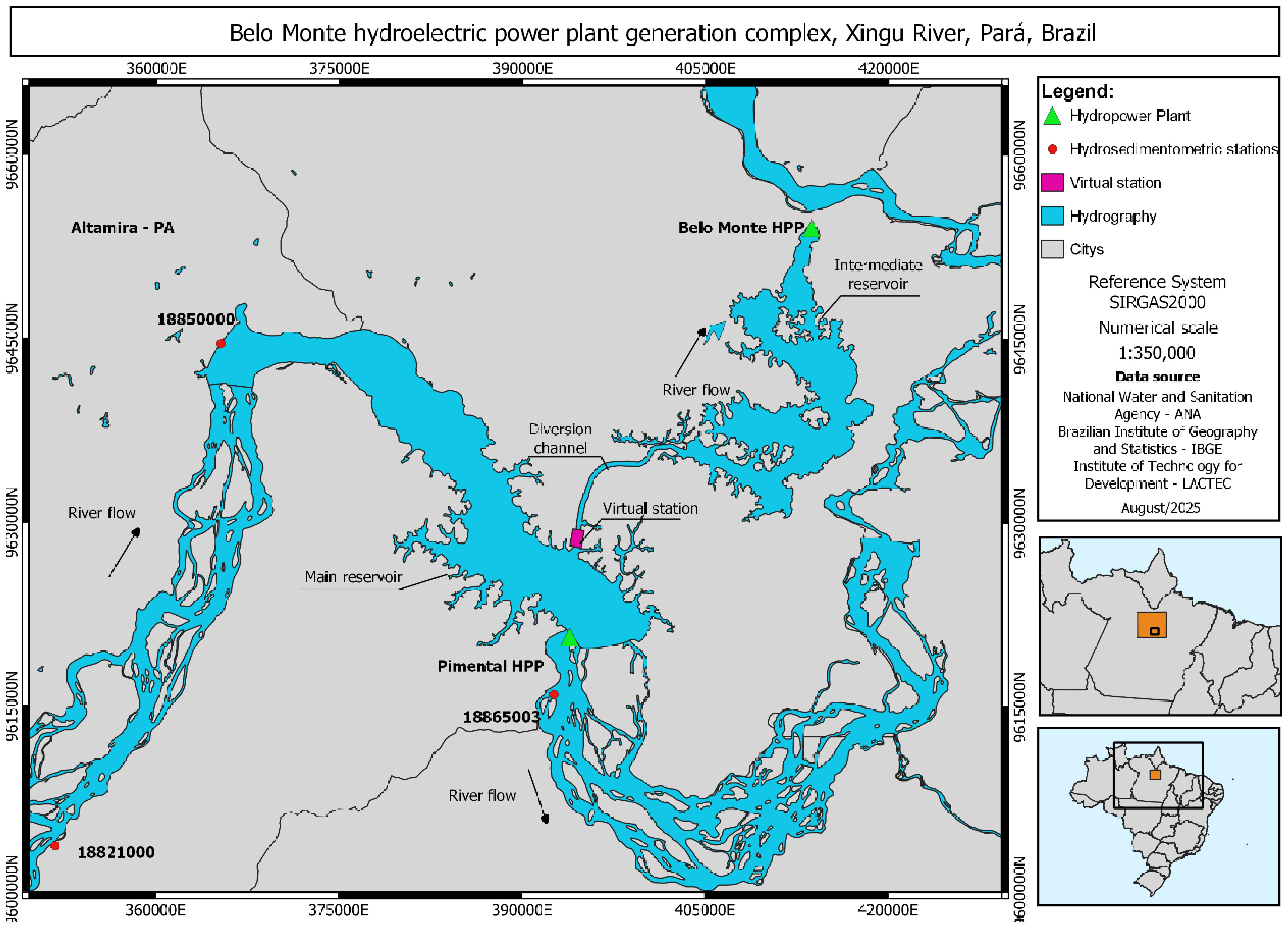
The study area is the Pimental HPP reservoir, which is the main reservoir of the Belo Monte HPP complex. The HPP complex is located on the Xingu River, in the Volta Grande do Xingu region, in southwestern state Pará, Brazil.

The Complex is formed by Belo Monte HPP (11,000 MW) and Pimental HPP (233 MW), with two reservoirs – the intermediate reservoir (119 km²) and the main reservoir (359 km²), respectively. The main reservoir is the focus of this work, as it is shown in Figure 1. Both reservoirs are connected by a diversion channel (20 km). The operation of this HPP Complex started in January 2016 (Norte Energia, 2024).

Figure 1
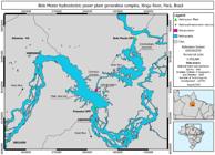
Location of the study area with the main fluviometric monitoring stations used in the study (upstream: 18821000 (UHE Belo Monte Montante) and downstream Pimental HPP: 18865003 (UHE Belo Monte Mangueiras).

Data considered in this paper was provided by Norte Energia SA and consisted of a hydrosedimentometric database, with data of water level elevation, discharge, rating curve, cross-sectional profiles, concentration of suspended sediment, among others, for stations located in the interest region. For this paper and analysis, datasets of the station 18821000 (UHE Belo Monte Montante), located upstream of the complex and station 18865003 (UHE Belo Monte Mangueiras), located downstream of the Pimental HPP were used. It is worth noting that the frequency of monitoring of suspended solids concentration on a monthly scale is higher than that commonly monitored in Brazil. The location of these stations is shown in Figure 1. The sedimentometric data was estimated using the solid discharge curves established for the stations 18821000, 18865003 and for the virtual station named diversion channel, as in Table 1.

Table 1
Sediment rating curve coefficients equation for stations 18821000, 18865003, and diversion channel. The equation is Q_ST=a Q_Liq b, in which Q_ST = Total solid discharge (t/d); Q_Líq = Liquid discharge (m³/s); a and b = coefficients of the equation.

Station	Coefficient a	Coefficient b	Source
18821000	0.180946	1.2535	Luz et al. (2025a)
18865003	0.019441	1.4997	Luz et al. (2025a)
Diversion channel	0.654900	1.0738	Luz et al. (2025b)

• Source: Luz et al. (2025a, 2025b).

The measured operation data was used to represent the outlet flows (flow through turbines, spillway and diversion channel) and the water level measurements defining the boundary condition of the spilled flows from Pimental.

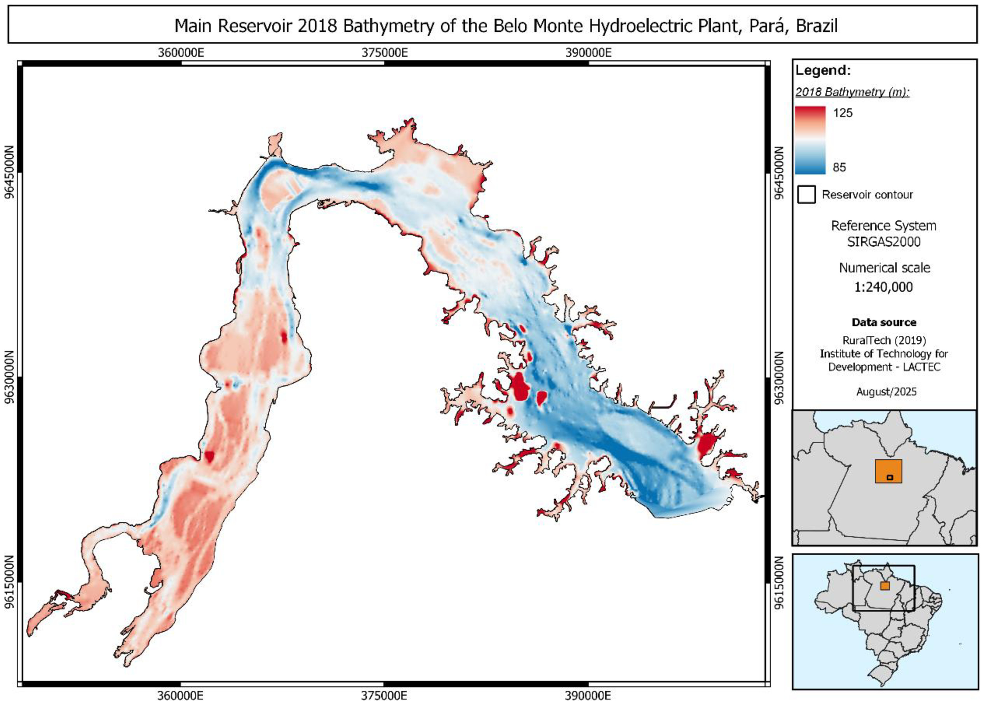
In addition, bathymetric data and depth-area-volume (DAV) curves were also provided by Norte Energia, which survey was performed after the start of operation (2018) (Ruraltech, 2019). Bathymetric measures were performed each 300 m of the reservoir and were used to define the initial bathymetry for the modeling.

Future scenario analysis (2018 to 2039)

To evaluate the medium-term sediment estimate (15 years), it was necessary to estimate future inflows and outflows into the reservoir. This was done based on flood studies provided by Norte Energia and using the observed flows from stations 18821000 and 18865003 (period from January 1, 2016, to May 9, 2024) to define a future hydrograph (May 10, 2024, to September 30, 2039). The hydrograph shape was obtained by averaging the annual hydrographs observed at the site. First, the hydrographs were normalized by the peak value, and then the average of the normalized hydrographs was obtained. Finally, the average hydrograph was multiplied by the desired peak value (corresponding RT).

The composition of this hydrograph was given by 3CMA, RT5, 3CMA, RT10, 4CMA, RT5, and 2CMA, where CMA is the hydrograph of an average flood, RT5 is the flood hydrograph with a 5-year return period (RT), and RT10 is a flood hydrograph with a 10-year return period (Intertechne, 2020a).

This arrangement was made because the period of interest was 15 years and, therefore, should include a hydrograph equivalent to a 10-year RT, at least two hydrographs equivalent to a 5-year RT, and for the remaining years, the average hydrograph was used.

It should be noted that changes in land use and occupation, the effects of climate change or other factors that may alter the distribution of flows and the contribution of sediment in the basin may be considered; however, this was not the focus of this article, thus not included.

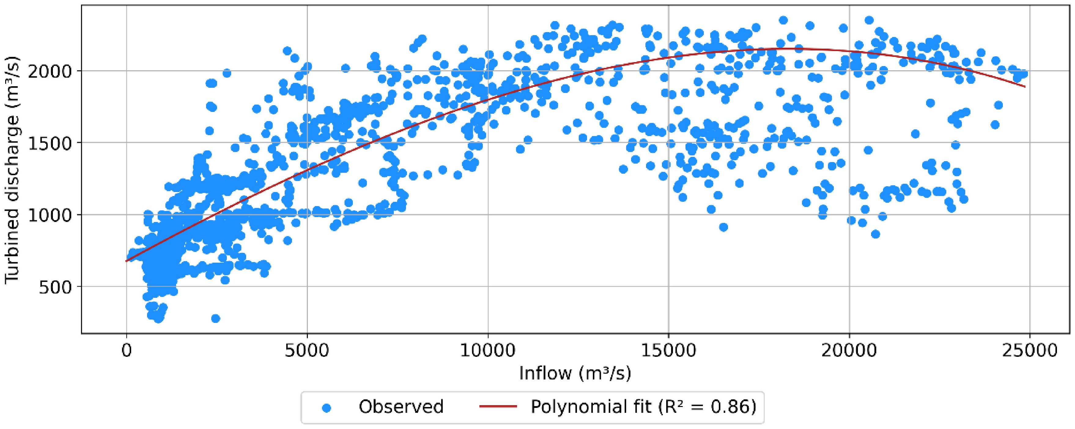
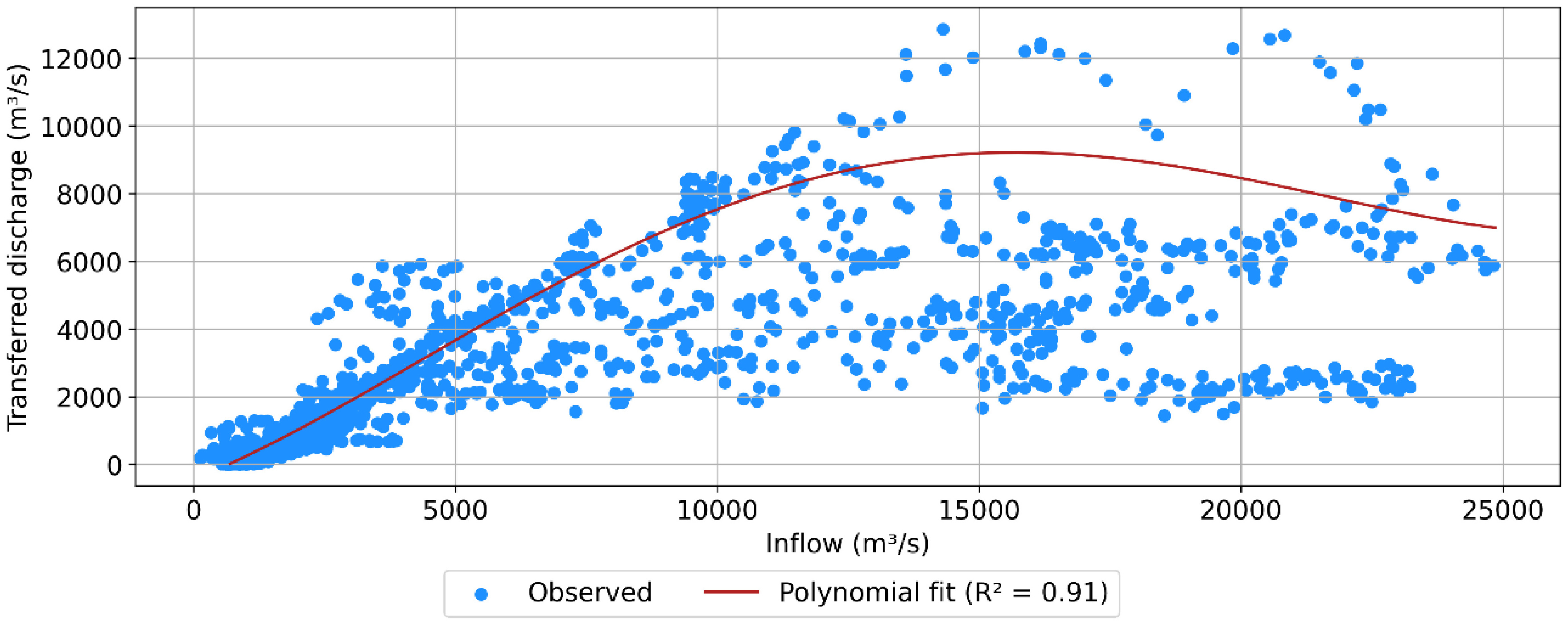
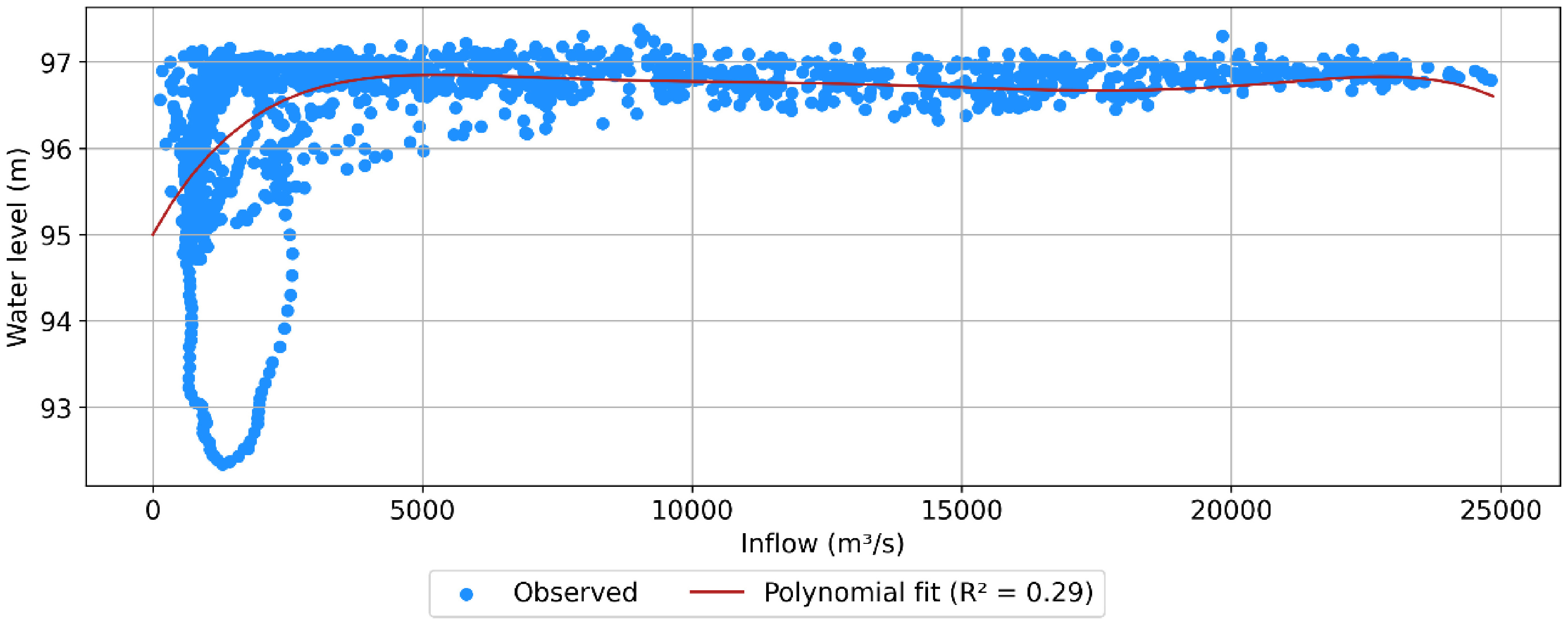
To define future operational flows, a polynomial trend-fit analysis was performed between station 18821000 and the corresponding structure (turbines, spillway, and diversion channel) for the observed data period. Subsequently, the future hydrograph was used to estimate future operational flows. It should be noted that for the spillway, the relationship used was based on the dam water level.

Sedimentometric method (mass balance)

Considering the flood study carried out for the Pimental HPP reservoir (Intertechne, 2012, 2020a), the occurrence of flow records and suspended solids concentration monitoring were evaluated and classified according to the flow magnitude. This was done to demonstrate the distribution of the available data for the application of this method.

Together with the discharge data (11/06/2018 to 09/05/2024) and the future data obtained from 10/05/2024 to 30/09/2039 in Future scenario analysis (2018 to 2039), historical series of solid discharge were estimated using the solid discharge curves established for the stations 18821000, 18865003 and for the virtual station named diversion channel, according to Luz et al. (2025a, 2025b) to close the mass balance, using the Colby Method (Colby, 1957).

It should be noted that changes in land use and occupation, climate change or other factors that may alter the solid discharge curve of the stations may be considered, however, this was not the focus of this article, thus not included.

For each station, the solid discharge values were evaluated in total terms per year and accumulated daily values. Thus, the deposited mass was determined through cumulative analysis using a mass balance approach, in which it was calculated by input (18821000) minus output (station 18865003 plus diversion channel station). Finally, the deposited volume was determined through the soil's apparent specific mass.

Simplified model Sediment

The Sediment model is a computational tool developed to estimate reservoir silting over time using simplified empirical methods (Braga, 2005). Based on the methodology of Borland & Miller (1958), it calculates the annual volume of deposited sediment and updates reservoir area-volume curves accordingly. The model incorporates key sedimentation processes, such as the apparent specific weight of deposited materials (Lara & Pemberton, 1963), sediment retention efficiency (Brune, 1953; Churchill, 1948), and sediment grain size distribution. It is used for long-term sedimentation analysis due to its practical input requirements and ease of implementation (Luz et al., 2025a).

Using the discharge data from station 18821000 available since 2011, together with the data estimated in Future scenario analysis (2018 to 2039), the average liquid discharge (7610 m³/s), the solid discharge series – using the same solid discharge curves (Luz et al., 2025a) – and the annual average solid discharge were calculated (5,433,125 t/year). These data are input to the model, as are grain size composition (24% clay, 32% silt, 44% sand), and a 2% annual increase in sediment load. Considering the initial volume as null, the reservoir water volume at the maximum normal water level (2022 hm³ at the 97.0 m elevation) and the average Brune curve, simulations using Sediment covered the period from 2018 to 2039, resulting in silting volumes for each year.

Hydrodynamic and sediment transport model description

Hydrodynamic modeling aims to better understand water dynamics (time series of levels and velocities and profiles and maps of level and velocity fields) and the representation of sediment transport (time series of concentrations and maps of concentration, erosion and sedimentation) and which in turn will provide indications of the silting process of the Pimental reservoir, an integral part of the Belo Monte HPP.

To achieve the objectives, the provided data were preliminarily analyzed, and it was observed that the simulation must be capable of representing hydrodynamic processes in a river regime and with three-dimensional resolution. For this purpose, the Delft3D model was chosen due to its large number of integrated applications (hydrodynamics and sediment transport), and being an open-source model. The Delft3D package was developed by Deltares in the Netherlands and consists of several modules, each with a different simulation focus. In this article, the hydrodynamics module (FLOW) was used.

The hydrodynamic module (Deltares, 2025) solves the transient shallow water equations, that are, a system formed by the mass balance and momentum equations for free surface flows. It assumes a hydrostatic pressure distribution, which disregards accelerations in the vertical direction. The other assumptions adopted in the mathematical formulation of the model are: the continuum hypothesis; incompressible flow; and the Boussinesq hypothesis, which consists of considering the flow acceleration to be less than that of gravity and, therefore, density variations are only important when they affect gravitational terms and not inertial terms.

Turbulence is solved through Reynolds decomposition and has four closure models for the vertical profiles: constant coefficient, algebraic method, κ-L model and κ-ε model (Deltares, 2025). This work used the κ-ε model because it is a more accurate model than the others. In the horizontal, constant eddy diffusivity values are used, as grid sizes are usually not capable to resolve small-scale turbulent structures. The value used here was 1 m²/s.

For sediment transport and morphological change calculations, the model calculates the concentration of suspended sediments and bed transport, as well as exchange processes at the water-bed interface (erosion and sedimentation) that result in accumulation or reduction of material at the bed. The model allows for the simulation of different sediment fractions, which can be cohesive and non-cohesive. The numerical model includes hydrodynamic changes due to bottom morphological changes and vice versa during the hydrodynamic calculation in a fully coupled manner (Deltares, 2025). For more information, see Deltares (2025).

Definition, calibration and validation of the hydrodynamic model

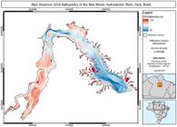
The modeling was performed by defining a three-dimensional grid based on the bathymetry for the Pimental reservoir, which used the reservoir contour and bathymetric data from 2018, provided by Norte Energia. To define the bathymetry of the numerical model, data from single-beam bathymetry carried out by Ruraltech (2019) in the Pimental reservoir were used. Figure 2 presents the original data (single-beam bathymetry) used to obtain the physical closed boundary condition (bathymetry) of the model.

Figure 2
Bathymetry of 2018 measured every 300 m (Source: Ruraltech, 2019).

The open boundary conditions used were the discharge time series from station 18821000 (upstream), the discharge transferred to the Belo Monte HPP (diversion channel), and the water level at the dam for the spillway (downstream). The turbined flow (powerhouse) was considered as a forcing factor in the model, since the turbine process occurs below the water surface and must be represented as such in the hydrodynamic model. Therefore, the turbine flow was included in the reservoir bottom layer as a discharge with negative values.

The modeling time step was defined, as well as the physical parameters of the model (Table 2). In the calibration process, the Manning coefficient was adjusted and a spatial distribution has been defined for it over the hydrodynamic grid (showed in the results section).

Table 2
Physical parameters of the three-dimensional hydrodynamic model

Parameter	Value	Unit
Gravity acceleration	9.81	m/s2
Specific mass of water	1000	kg/m3
Horizontal eddy viscosity	1	m2/s
Vertical background eddy viscosity	3D Turbulence Model - k- Epsilon	-
Time step	30	s

Reports from previous studies using 1D and 2D steady-state models (in which measurements were also available) were used to compare the results for long-term average flow rates and with a 5-year TR (Intertechne, 2020a, 2020b). This was done considering that in the Pimental HPP backwater studies, field measurements were also taken and used to calibrate the HEC-RAS and RiverFlow2D models, thus ensuring that both simulations can be used to calibrate other models.

For calibration, the water levels at the Altamira Trapiche fluviometric station (18850000) (Figure 1) were used through the rating curve (with reservoir) obtained from Intertechne (2020b). A visual comparison of the velocity and water level maps was also carried out for the flows of 8,045 m³/s and 26,224 m³/s, respectively.

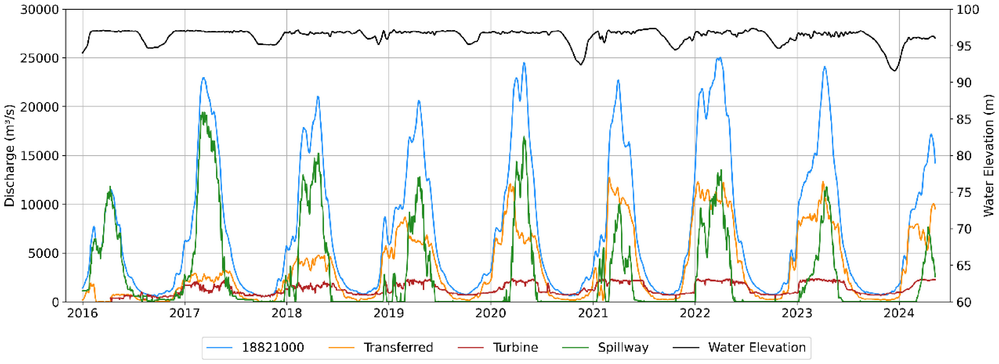
After verifying the quality of the model (calibration), simulations were carried out for the period between 06/11/2018 and 05/09/2024. The data used for this period were the discharge data from the upstream station (18821000) which was used as the open boundary condition, as well as the discharge data on spilled and transferred flows (boundary conditions), turbine flows (discharge in the model) and reservoir level according to the history of this period (Figure 3).

Figure 3
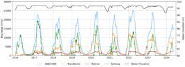
Flow rates at station 18821000, operating flows at Belo Monte HPP (transferred, turbined and spilled) and level up to 2025.

For this period, the verification of the hydrodynamic model was carried out based on the results of the Nash-Sutcliffe coefficient (NSE), which was evaluated in terms of simulated outlet flows and operational data from HPP Pimental.

Sediment transport model

Sediment transport modeling used as initial bathymetry the one from the 2018 survey, along with the flow and water level data described in the previous section. The simulated period was between June 11, 2018, and May 9, 2024.

The solid flow rates used were the same as those obtained for stations 18821000 and 18865003 in Sedimentometric method (mass balance). The model considered the non-cohesive and cohesive fractions, which represent 60% and 40% of the total solid discharge, respectively (Intertechne, 2011). A D₅₀ diameter of 480 µm was adopted in the simulation for non-cohesive sediment, in agreement with granulometry information provided by Norte Energia. The initial sediment thickness in the reservoir for the cohesive and non-cohesive fractions was set to 0 m, and the initial concentrations in the reservoir was set to 7.63 mg/L for the cohesive fraction and 11.45 mg/L for the non-cohesive fraction, distributed uniformely over the entire reservoir. It should be noted that there are no measurements available in the reservoir for suspended and bottom sediment concentrations or transport measurements.

To verify the quality of the modeling, the results from the suspended sediment concentration at the location of the diversion channel were compared with estimated values from literature (Luz et al., 2025b), which were obtained through satellite image analysis, given that there are no available measurements of sediment concentration in the reservoir. The period used in this step coincides with June 11, 2018, and May 9, 2024.

To estimate the silted volume, two methods of calculating the mass balance were used, based on the results obtained by the Delft3d model. The first was by exporting the accumulated volumes calculated by the hydrodynamic model at the locations of the open boundary conditions by total cumulative transport (in this article, referred to as method 1). The second was by estimating the loads at the inlet and outlet (method 2) from the concentrations and flow rates (i.e., Load = QC, where Q is the flow rate in m³/s and C is the concentration in mg/L).

For the powerhouse, however, the load was calculated and subsequently converted to volume (using the default value of the model for the reference density of 1600 kg/m³), given that this output was considered a discharge and therefore did not allow the definition of a cross-section for controlling the total cumulative transport.

After calibration and verification, a simulation was performed considering the future period 06/11/2018 to 09/30/2039.

RESULTS AND DISCUSSION

Future scenario analysis (2018 to 2039)

The hydrograph composition was 3CMA, RT5, 3CMA, RT10, 4CMA, RT5, 2CMA in which CMA is the hydrograph of an average flood, RT5 is the flood hydrograph with a return time (RT) of 5 years and RT10 a flood hydrograph with a return time of 10 years, whose flood studies are available in Intertechne (2020a).

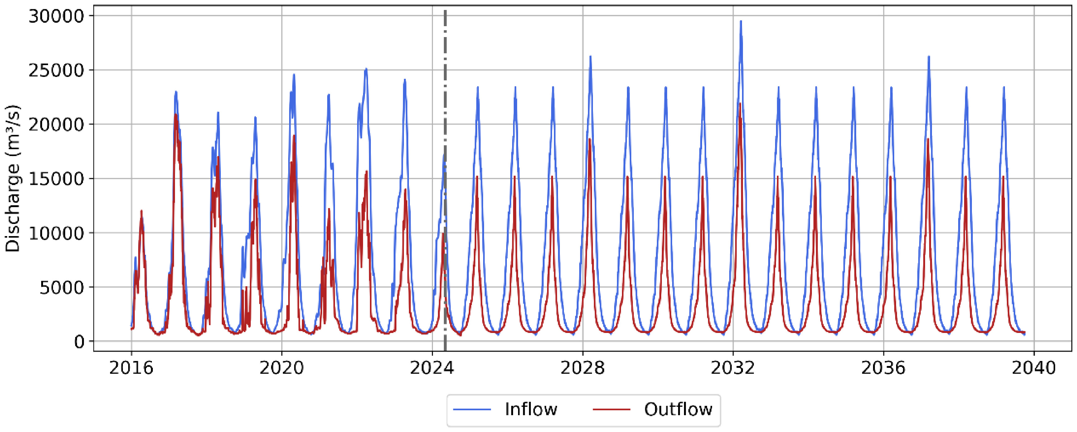
From the composition of the hydrograph for the future period (May 10, 2024, to September 30, 2039), the reservoir inflow and outflow rates were obtained by the polynomial trend-fit analysis, as shown in Figure 4. It can be seen that the future flows present less noise compared to the observed data, which was expected, since they were obtained from average hydrographs.

Figure 4
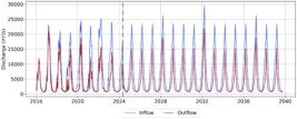
Flow series from the medium-term scenario simulation for the Pimental Reservoir. The gray vertical line indicates the division between observed and future data.

Camargo (2019) also generated future flow series for the Xingu River in the Belo Monte HPP region for the period 2020-2050, however using precipitation projections from five CMIP5 climate models (RCP8.5 scenario). This study assessed the potential impacts on power generation from the Belo Monte HPP. Saboia et al. (2025) used climate change projections based on CMIP6, from which flows were obtained for all basins of the National Interconnected System (SIN). However, it should be noted that assessing climate change in siltation is not the objective of this article.

The future series of turbine flow at HPP Pimental and flow transferred to HPP Belo Monte, and the dam level data (spillway) were obtained from the future hydrograph and the polynomial trend adjustment analysis as illustrated in Figure 5, Figure 6 and Figure 7, respectively.

Figure 5
Relationship between turbine flow and inflow to the Pimental reservoir.

Figure 6
Relationship between flow diverted by the canal and flow inflow to the Pimental reservoir.

Figure 7
Relationship between reservoir water level and inflow to the Pimental reservoir.

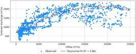
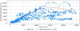
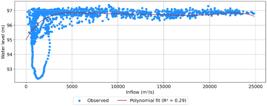
For the turbine flow (Figure 5 and Equation 1), the trend curve was used up to the maximum turbine swallowing and kept constant at 2,152 m³/s. The quality of the fit was defined using the R², which was 0.86. For the flow transferred through the diversion channel (Figure 6 and Equation 2), the trend curve was used up to its maximum value (9,150 m³/s) and kept constant for values above that. For the dam level (Figure 7 and Equation 3), the trend curve was used up to its maximum value (96.94 m) and kept constant for values above that.

It is important to highlight that energy generation at Belo Monte HPP increased gradually starting in 2016, with the activation of several generating units at different times. Therefore, its full operating capacity took several years to be reached. Thus, when adjusting the transferred flow rate to the inflow rate to the reservoir, for example, for higher inflow rates, there is a greater dispersion of transferred flows. Therefore, priority was given to adjusting the flow rate considering higher transferred flows for higher inflow rates.

$-7.15{10}^{-11}{x}^3-1.77{10}^{-6}{x}^2+1.37{10}^{-1}x+676$ (1)

$\begin{array}{c}1.20{10}^{-13}{x}^4-6.23{10}^{-9}{x}^3+6.76{10}^{-5}{x}^2+\\ 6.25{10}^{-1}x-445\end{array}$ (2)

$\begin{array}{c}7.6{10}^{-25}{x}^6+6.1{10}^{-20}{x}^5-1.9{10}^{-15}{x}^4+\\ 3.1{10}^{-11}{x}^3-2.6{10}^{-7}{x}^2+1.1{10}^{-3}x+9.5\end{array}$ (3)

Sedimentometric method (mass balance)

Based on flood studies (Intertechne, 2020a), flow records and suspended sediment concentration measurements from station 18821000 were quantified. It was observed that even in 13 years of data, there are no records of flows equivalent to or greater than events with a RT greater than 10 years. Regarding suspended sediment concentration measurements, there were even fewer measurements, which occurred only once and in an event with a RT equivalent to 5 years (Table 3 and Figure SP 1), that is, only one measurement was performed in the interval between the CMA flow and the RT5 flow. This suggests a limitation of suspended sediment monitoring data during flood peaks, that is, at times when sediment transport is greatest, which can produce underestimated results on the solid discharge. Even so, its use is not discouraged, and its application was carried out.

Table 3
Net flow records and suspended sediment concentration measurements from station 18821000 by flow interval.

Return times	Flow rate (m3/s) 1	Flow records	Sediment measurement
MMA2	Until 999	492	17
MLT3	8,045	2,639	71
CMA4	23,368	1,755	41
RT 5	26,224	34	1
RT 10	29,472	11	0
RT 25	33,766	0	0
RT 50	37,014	0	0
RT 100	40,262	0	0
RT 1000	51,052	0	0
TR 10000	61,842	0	0

• Note: 1 – Intertechne (2020a); 2 – average of annual minimums; 3 – historical average; 4 – average of maximum annual flows.

Using the liquid discharge obtained in Future scenario analysis (2018 to 2039) and the solid discharge curve (Table 1), the solid discharge series of each station was calculated and daily accumulated. The reservoir sedimentation estimates were calculated by the difference in accumulated mass between the output (stations 18865003 plus diversion channel station) and the input (station 18821000), as in Table 4.

Table 4
Estimated volume of accumulated sediment from 2018 to 2039 at Pimental HPP.

Date	Accumulated solid discharge (10 6 t/d)			Accumulated volume in the year (hm3)
	Input	Output	Input - Output
	18821000	18865003 + Channel
12/31/2018	0.76	0.51	0.24	0.20
12/31/2019	5.60	4.14	1.46	1.20
12/31/2020	11.28	8.57	2.72	2.23
12/31/2021	16:45	12.09	4.36	3.59
12/31/2022	23.83	17.41	6.42	5.28
12/31/2023	29.43	21.33	8.09	6.66
12/31/2024	33.23	23.95	9.28	7.64
12/31/2025	38.69	27.63	11.06	9.10
12/31/2026	44.14	31:30	12.84	10.56
12/31/2027	49.68	35.04	14.63	12.04
12/31/2028	55.91	39.56	16.36	13:45
12/31/2029	61.37	43.23	18.13	14.92
12/31/2030	66.82	46.91	19.91	16.38
12/31/2031	72.46	50.73	21.73	17.88
12/31/2032	79.59	56.26	23.32	19.19
12/31/2033	85.04	59.94	25.10	20.65
12/31/2034	90.50	63.62	26.87	22.11
12/31/2035	95.95	67.30	28.65	23.57
12/31/2036	101.51	71.06	30.46	25.05
12/31/2037	107.72	75.55	32.17	26.46
12/31/2038	113.18	79.23	33.95	27.92
09/30/2039	118.04	82.49	35.55	29.25

The results obtained indicated a sedimentation of 29 hm³ throughout the entire evaluated period, which is equivalent to a sedimentation rate of 1.37 hm³/year. This value corroborates the results obtained by Luz et al. (2025a) since the solid discharge curve equation used is coincident between both studies.

Sediment balance has been used in other studies for different purposes. Lemma et al. (2024), for example, used mass balance to assess the sediment retention efficiency of reservoirs. The authors considered the impact of reservoirs currently under construction and operation (scenario 1) and also included those in the planning phase (scenario 2). This study observed that, in scenario 1, sediment retention by dams led to a 15% reduction in the annual sediment load reaching Lake Tana (Ethiopia). In scenario 2, the sediment load reduction reached 52%, demonstrating the sediment retention efficiency of reservoirs (Lemma et al., 2024).

In Cachí reservoir (Costa Rica), the sediment balance was used to evaluate the efficiency of the flushing process (Jansson & Erlingsson, 2000). According to the sediment input, approximately 80% was retained in the reservoir between two flushing events (one year). After the process, approximately 71.4% of the input was released from the reservoir.

Simplified model Sediment

The simulation of the Sediment model yielded, for each year, the corresponding values of deposited solid volume, effluent solid volume, retention efficiency, specific weight, and influent and effluent solid discharges (Table 5). The total silted volume was estimated until 2039 to 50.3 hm³, which corresponds to a silting rate of 2.52 hm³/year.

Table 5
Sediment model simulation results from 2018 to 2039 at Pimental HPP.

Year	Solid volume deposited (hm3)	Effluent solid volume (hm3)	Retention Efficiency (%)	Apparent range (kg/m3)	Solid Q Influent (t/year) x 103	Q solid Effluent (t/year) x 103	Deposited solid volume/Total reservoir volume
2018	2.03	5.65	41.76	1142	5542	3228	0.001
2019	4.02	8.44	41.73	1164	5653	3294	0.002
2020	6.02	11.25	41.71	1177	5766	3361	0.003
2021	8.03	14.11	41.69	1186	5881	3429	0.004
2022	10.08	17.01	41.66	1194	5999	3499	0.005
2023	12.14	19.96	41.64	1200	6119	3571	0.006
2024	14.24	22.95	41.62	1206	6241	3644	0.007
2025	16.38	25.99	41.59	1210	6366	3718	0.008
2026	18.54	29.09	41.57	1215	6493	3794	0.009
2027	20.74	32.24	41.54	1218	6623	3872	0.010
2028	22.98	35.45	41.52	1222	6755	3951	0.011
2029	25.25	38.71	41.49	1225	6891	4032	0.012
2030	27.57	42.04	41.47	1228	7028	4114	0.014
2031	29.92	45.43	41.44	1231	7169	4198	0.015
2032	32.32	48.88	41.41	1233	7312	4284	0.016
2033	34.75	52.39	41.38	1236	7459	4372	0.017
2034	37.23	55.98	41.35	1238	7608	4462	0.018
2035	39.75	59.63	41.32	1240	7760	4553	0.020
2036	42.32	63.35	41.30	1242	7915	4647	0.021
2037	44.93	67.14	41.26	1244	8073	4742	0.022
2038	47.60	71.00	41.23	1246	8235	4839	0.024
2039	50.30	74.95	41.20	1247	8400	4939	0.025

The retention efficiency decreases from 41.7 to 41.2%, corroborated by the values obtained for effluent solid discharge increases. The apparent specific weight of the soil obtained was 1,216 kg/m³, which was close to that achieved by Luz et al. (2025a) also with Lara & Pemberton (1963) method. This value is lower than the reference value adopted in the 3D modelling. Since there are no measurements of specific weight in situ, these values ​​were considered in their respective simplified model and 3D modeling applications.

Another study also used the Sediment model to estimate siltation in the Pimental HPP reservoir (Intertechne, 2011), in which, up to the 22nd year of simulation, 39 hm³ were obtained, a result 21% lower than that obtained in the present study. This difference may be linked to the fact that the average annual inflow data for liquid and solid discharge to the reservoir used were respectively higher and lower than those used in the present study.

Hydrodynamic and sediment transport modeling

Definition, calibration and validation of the hydrodynamic model

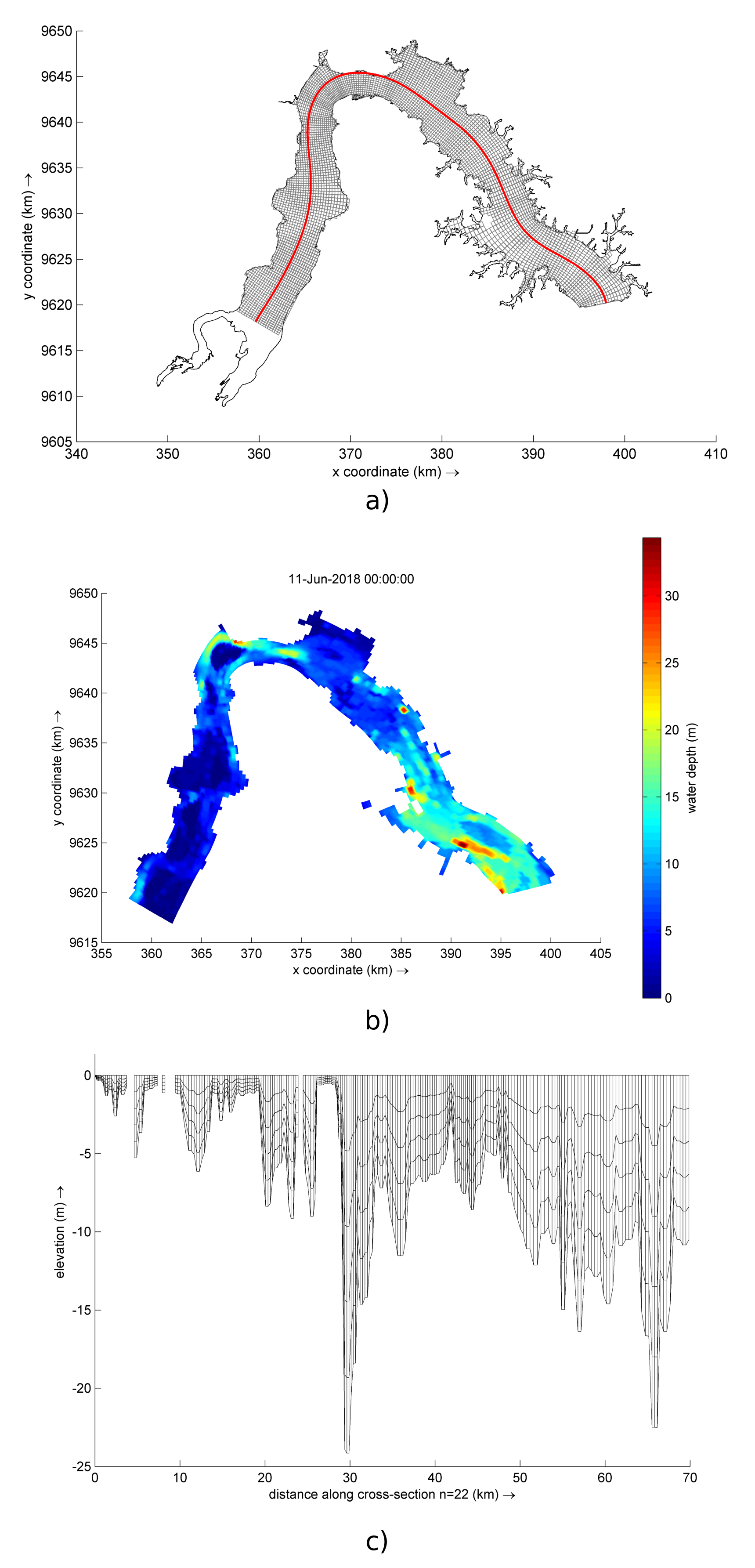
The model was initially defined using the computational grid (Figure 8a), a three-dimensional sigma grid with five equally distributed depth layers, with cells measuring between 136 m and 650 m in horizontal resolution. Figure 8b shows the bathymetry interpolated over the model grid. Figure 8c shows a longitudinal section of the computational grid and its vertical distribution. With the used 30s time step, the Courant criterion (Courant<10) (Deltares, 2025) was met.

Figure 8
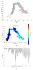
(a) Computational mesh – general view; (b) Initial bathymetry provided by topo-bathymetric data – water depth below the water level interpolated for modeling (the water level considered is around 97.50 m); (c) Longitudinal section showing the vertical distribution of the layers in the red section in Figure (8a).

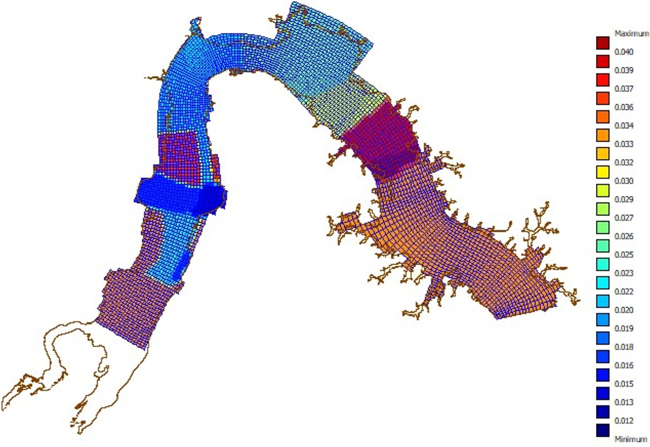
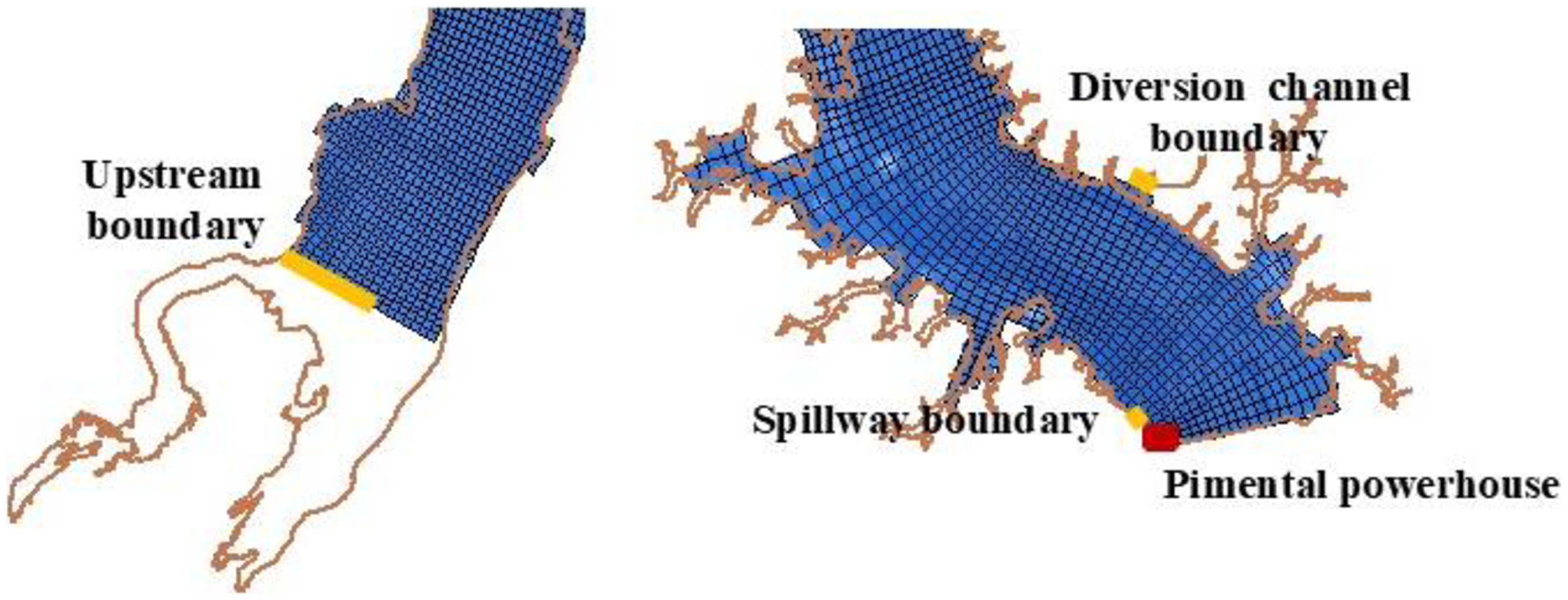
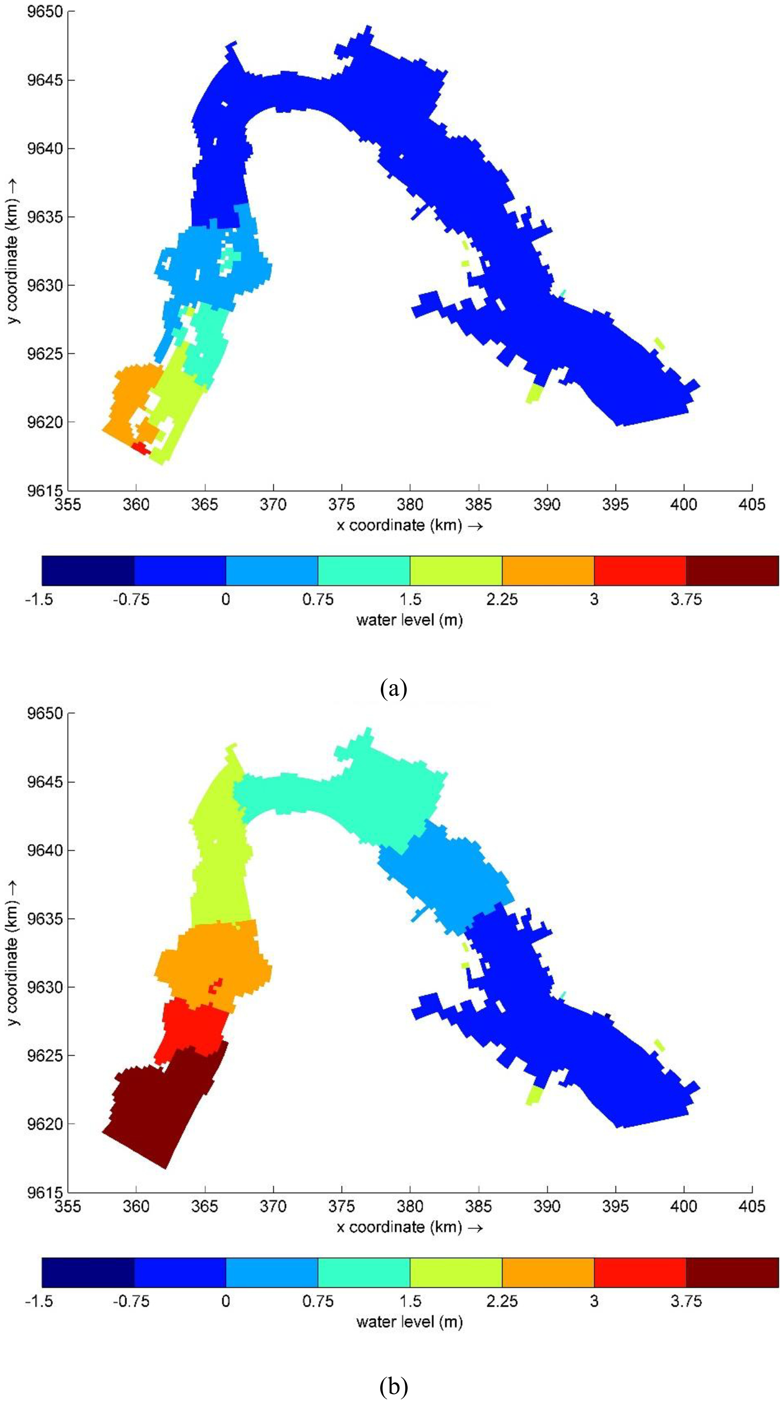
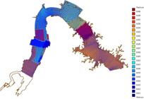
During calibration, the final Manning coefficient obtained varied spatially over the modeling domain, as shown in Figure 9, with values ranging from 0.01 to 0.04. The representation of the boundary conditions is shown in Figure 10, considering the inlet and outlets (spillway and diversion channel). The powerhouse, represented in the model as a negative discharge, is also shown in this figure.

Figure 9
Manning coefficient in the Pimental reservoir modeling domain.

Figure 10
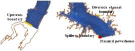
Upstream boundary condition (left), downstream boundary condition at the spillway and diversion channel (right) and powerhouse (discharge).

To evaluate the quality and accuracy of the hydrodynamic model in the calibration process, comparisons were made with previous studies with results from 1D and 2D models applied for steady flow studies and calibrated to measured data.

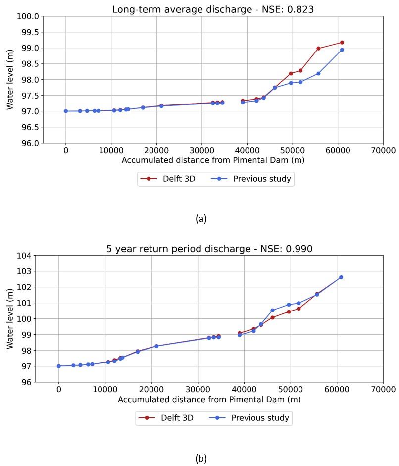
From the results obtained with the calibrated HEC-RAS 1D model (Intertechne, 2020a) for flows of 26,224 m³/s (flow in the diversion channel of 9,000 m³/s), corresponding to a 5-year return period (RT5), and 8,046 m³/s (flow in the diversion channel of 6,210 m³/s), corresponding to the long-term average flow a comparison was performed. The comparison for both flows is presented in Figure 11. Upstream of the urban area of Altamira (more than 40,000 m in the graph), the difference between the models is due to the fact that the previous study carried out in a 1D model and the modeling performed in the project is 3D, which is considered more suitable for the region that has many islands and a main flow not being parallel to the reservoir banks. In general, there is good agreement between the models, with Nash-Sutcliffe coefficient (NSE) resulting in 0.82 and 0.99, for long term averaged and RT5 discharges, respectively.

Figure 11
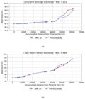
Water level comparison between HEC-RAS 1D and Delft3D model results for (a) MLT (8,046 m³/s) and (b) 5-year TR (26,224 m³/s) flow. The red line represents the calibrated model.

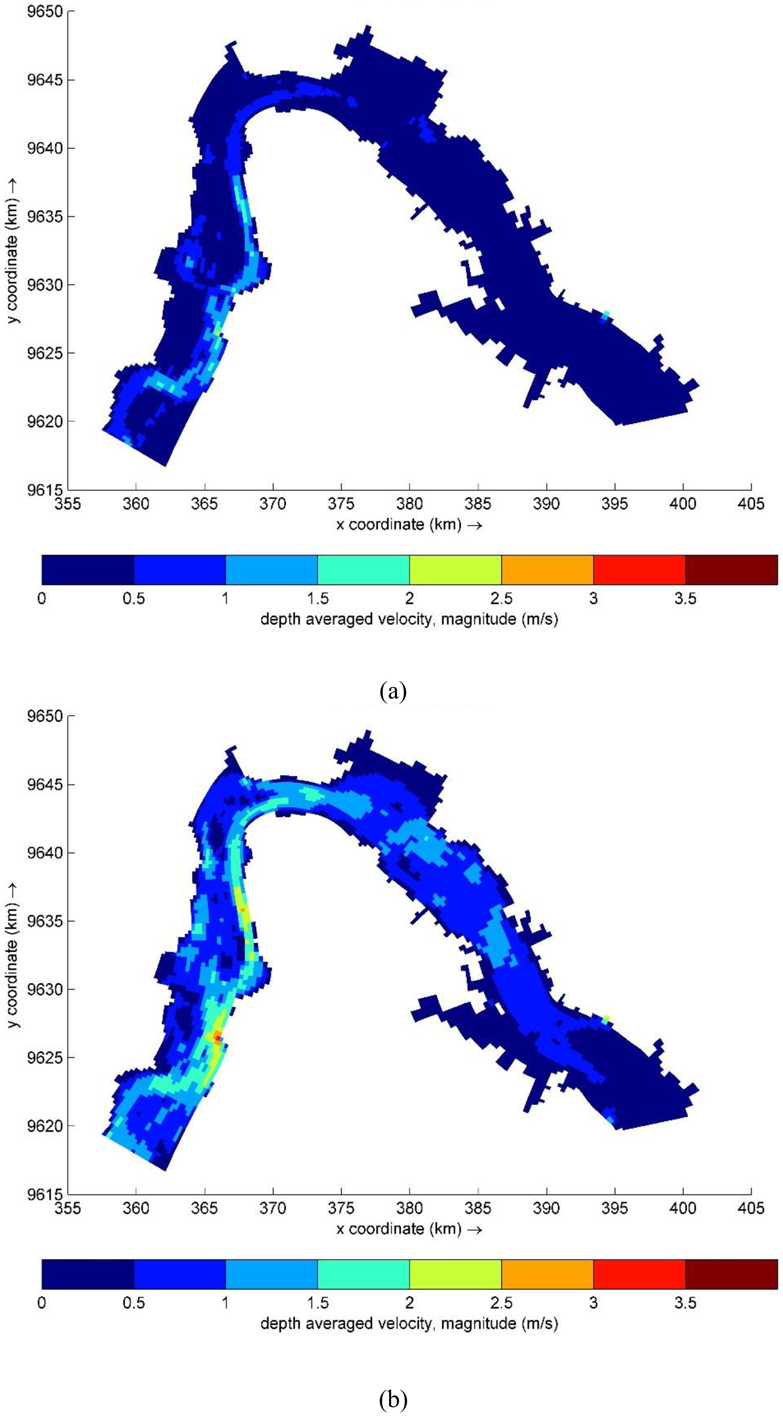
Using the results obtained with the calibrated RiverFlow2D model (Intertechne, 2020b), comparisons were initially made with measured data in Altamira, indicating differences on the order of centimeters between the measurements and the Delft3D model (Table 6). In this case, it was also possible to make comparisons between the flow rates of 8,045 m³/s and 26,224 m³/s. The velocity maps for the respective flow rates are presented in Figure 12 and Figure SP 2 (result of the RiverFlow2D model presented in the supplementary material). The water level maps are presented in Figure 13 and Figure SP 3. In both cases, it was possible to observe that the Delft3D model reproduces orders of magnitude of velocity and water level similar to those obtained by the RiverFlow2D model.

Table 6
Comparisons between modeling results (Delft3D) and data measured in Altamira.

Flow rate Influent (m 3 /s)	Belo Monte flow rate (m 3 /s)	Elevation in Altamira (m)
		Key curve1	Simulation	Difference
5,000	3,663	97.08	97.13	0.05
10,000	7,521	97.37	97.47	0.10
15,000	9,000	97.84	97.94	0.10
20,000	9,000	98.52	98.44	-0.08

• Note: 1 – Intertechne data (Intertechne (2020b).

Figure 12
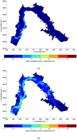
Average vertical velocity results in the Delft3D model. (a) Flow rate of 8,045 m³/s (MLT); (b) Flow rate of 26,224 m³/s (RT5).

Figure 13
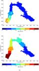
Water level results in the Delft3D model (in relation to the 97.5 m elevation). (a) Flow rate of 8,045 m³/s (MLT); (b) Flow rate of 26,224 m³/s (RT5).

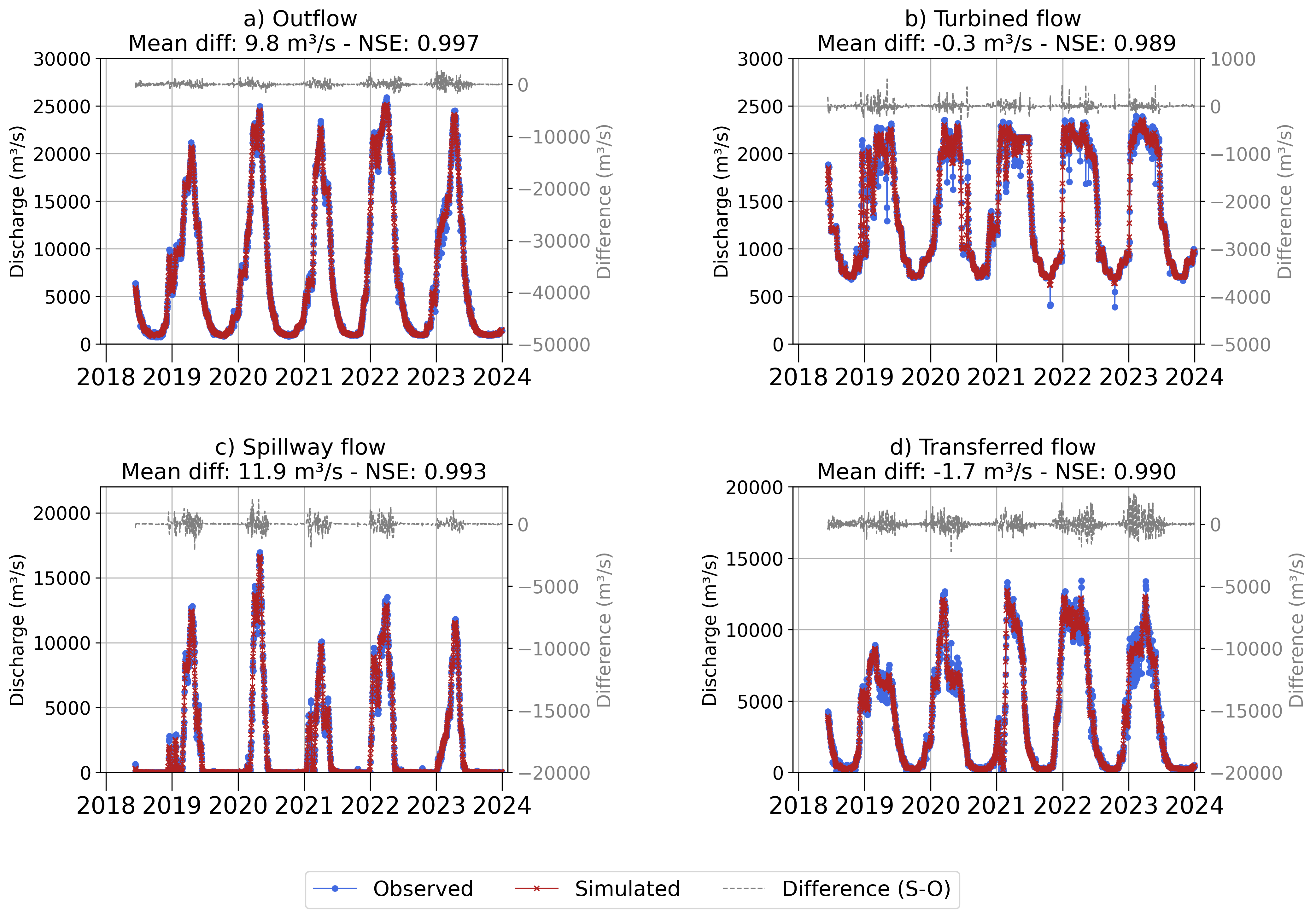
During the validation stage, the Delft3d model was simulated for the period from June 11, 2018, to May 9, 2024. The simulation results were compared with observed values to verify the modeling quality, namely: outflow, spillway, powerhouse, and transferred flow rates. Figure 14 shows the comparisons of the simulations with the measured outflow, turbine, overflow, and transferred flow rates, respectively, demonstrating an overlap between the observed and simulated series. Regarding the Nash-Sutcliffe coefficient (NSE), for the four flow rates evaluated, the coefficient ranged from 0.989 to 0.997, which corroborates the good performance of the simulation.

Figure 14
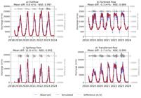
Comparison between the flow rate (a) effluent; (b) turbine; (c) spilled and (d) transferred measured and simulated by the Delft3D model.

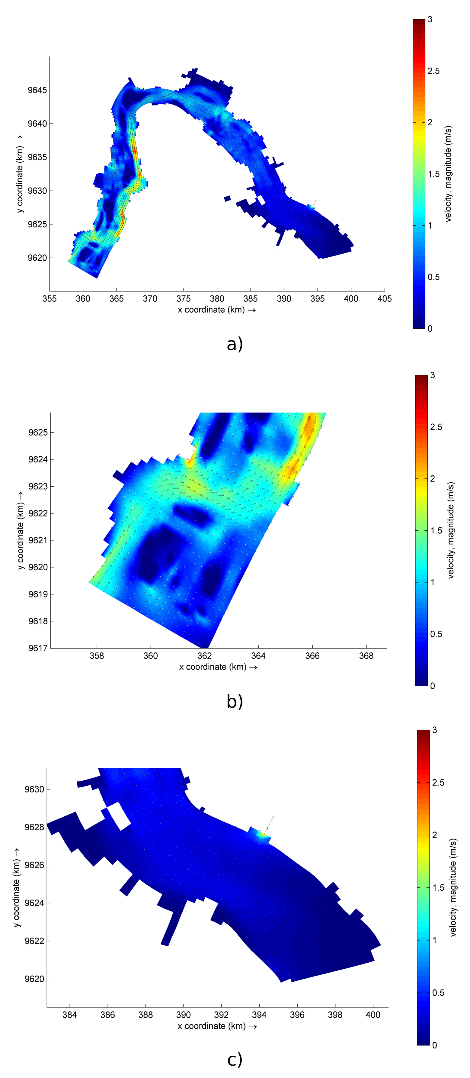
The simulations performed allowed us to observe some characteristics of the reservoir flow. Figure 15a presents the surface velocity magnitude map and velocity vectors at the surface and bottom of the Pimental Reservoir for May 9, 2024. This figure shows the highest velocities in the region from the reservoir inlet (zoomed in on Figure 15b) to the city of Altamira, which decrease after the bend in the Xingu River. In this region, no changes in velocity direction between the surface and the bottom are observed. Figure 15c presents the same results, but focusing on the diversion channel region, where there is a reduction in velocity along the Xingu River, but an increase in velocities within the channel itself.

Figure 15
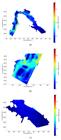
Map of average velocity magnitude and velocity vectors: white vector: surface velocity; black vector: bottom velocity for the date of 09/05/2024. (a) Entire simulated domain; (b) Focus on the reservoir inlet; (c) Focus on the diversion channel region.

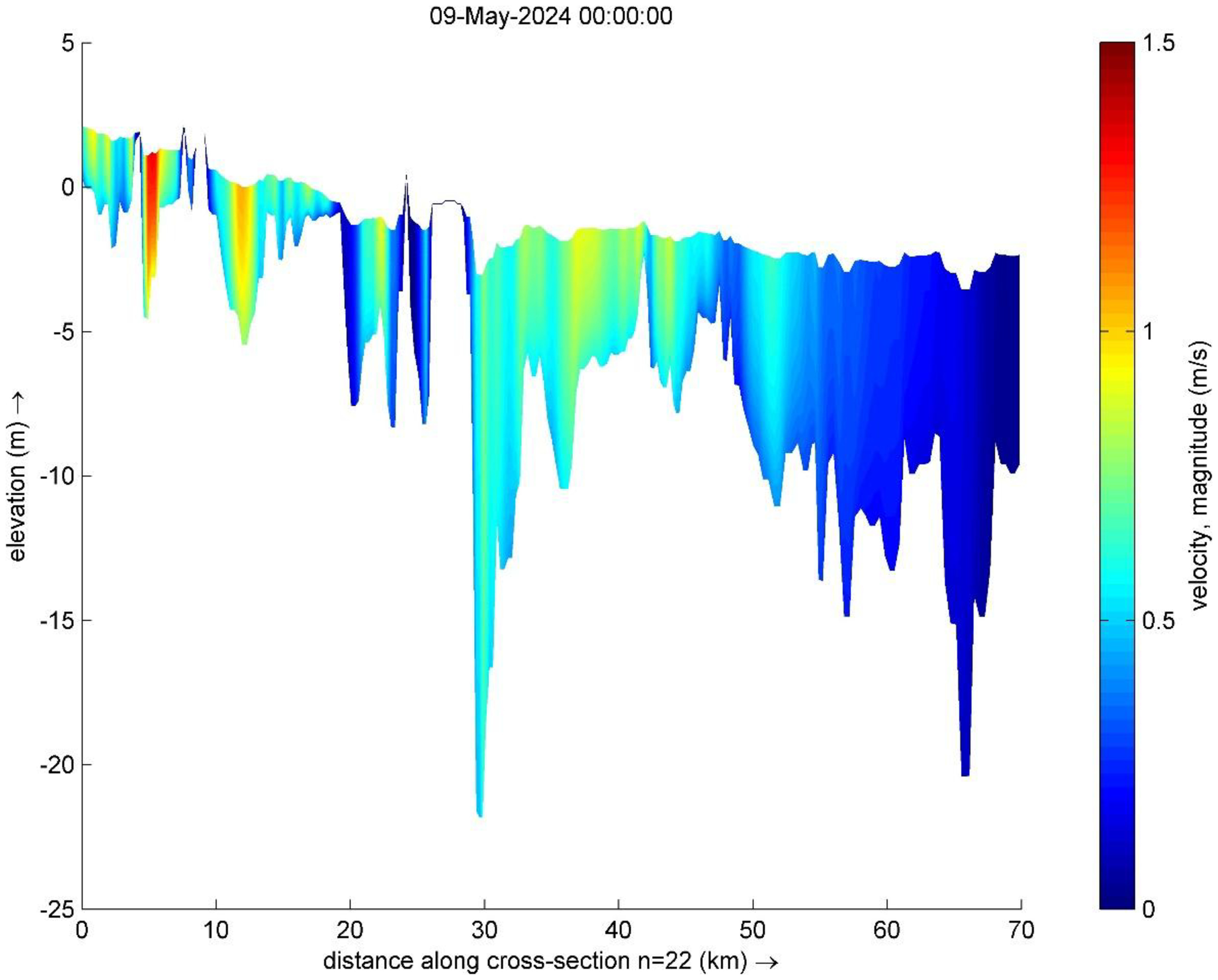
Figure 16 shows the velocities in a longitudinal section of the reservoir for the date of 09/05/2024. From the figure, velocities greater than 1 m/s were observed in the upstream region, while approaching the dam there is a reduction in velocities.

Figure 16
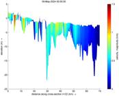
Longitudinal section (shown in Figure 8) with the average velocity magnitude of the Pimental reservoir for the date of 09/05/2024. Zero on the x-axis corresponds to the reservoir inlet.

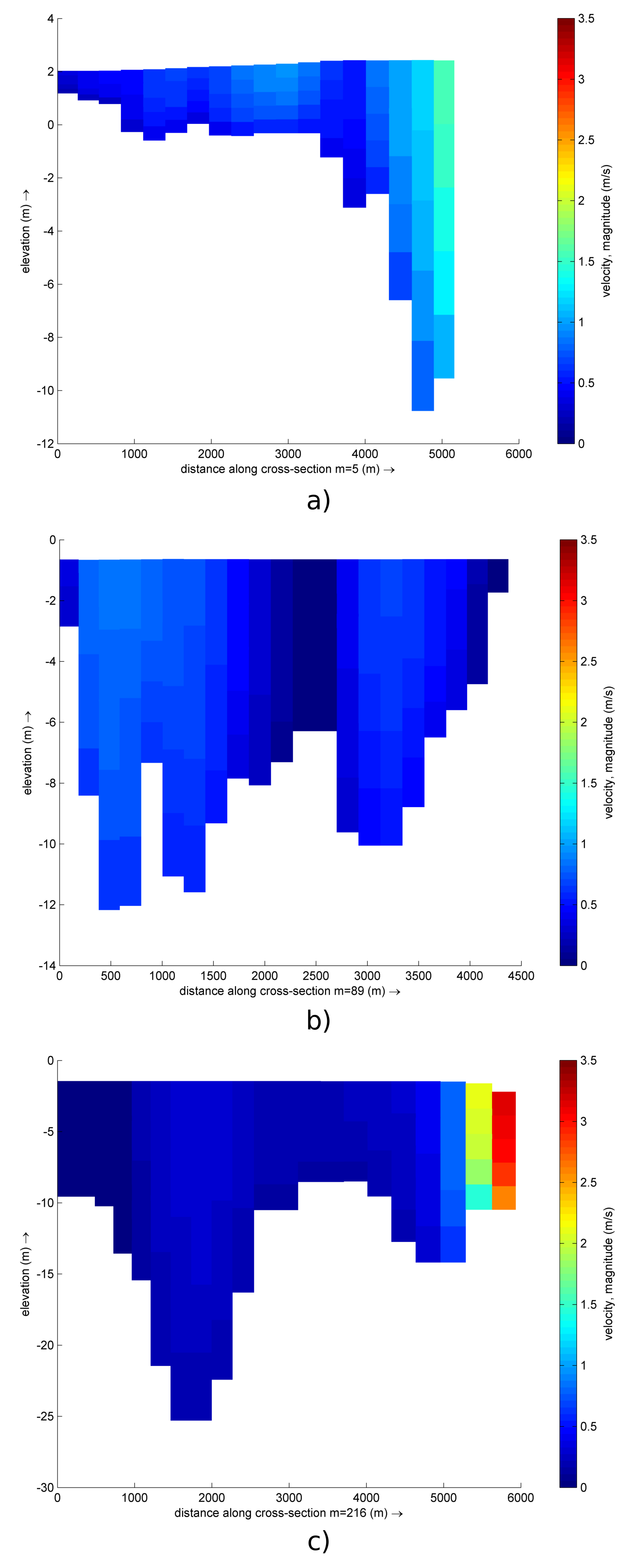
Figure 17 shows the velocities in three cross-sections: upstream, near Altamira, and the section contemplating the diversion channel, respectively, for the date of May 9, 2024. The upstream section (Figure 17a) presented velocities of up to 1.5 m/s in the river channel. In the Altamira section (Figure 17b), there is a reduction in velocities, as well as in the diversion channel section (Figure 17c), with the exception of the channel entrance, which presented velocities of up to 3 m/s.

Figure 17
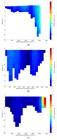
Velocity magnitude in the cross sections of the Pimental reservoir for the date of 09/05/2024. (a) Upstream section; (b) Altamira section; (c) Diversion channel.

Sediment transport model

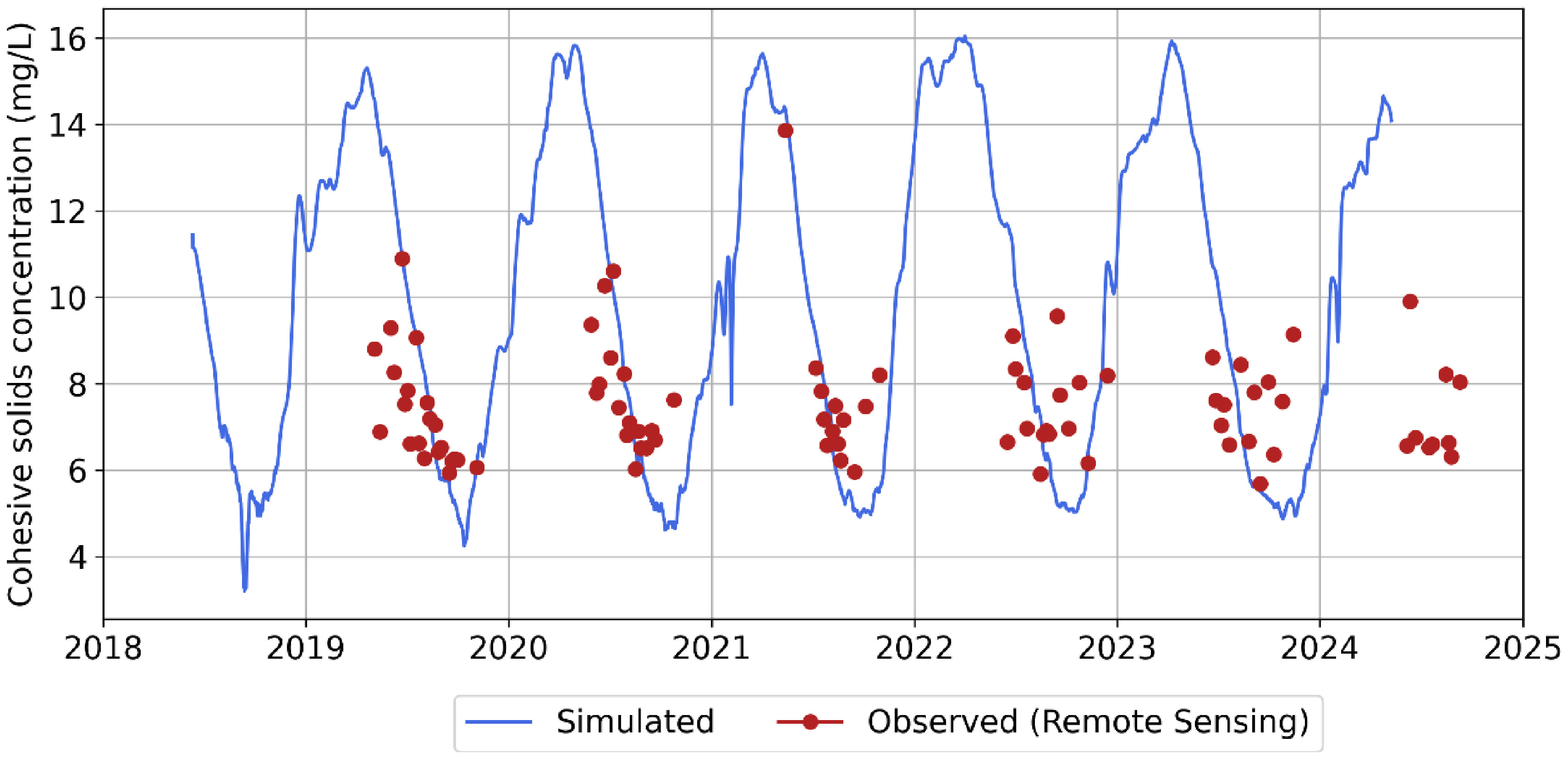
To verify the quality of the modeling results, comparisons were made between the simulated and estimated suspended sediment concentrations in the literature (Luz et al., 2025b) as shown in Figure 18. In this figure, it can be seen that there are no satellite images available during the flood period, but there are data on the rise and fall of the hydrograph, which were reproduced by the numerical model, with concentrations between 6 and 12 mg/L.

Figure 18
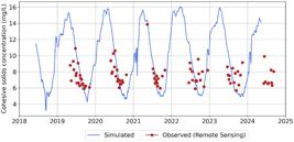
Comparison between simulated and satellite imagery cohesive sediment concentration for the diversion channel.

To estimate the silted volume through modeling, the results of the total cumulative transport were exported for the model's boundary conditions, which are represented in Figure SP 4. The largest sediment accumulations occur due to the flood periods.

Table 7 presents the sediment volume results from the mass balance for methods 1 and 2. For method 1, a siltation of 7.17 hm³ was estimated by the mass balance in the period 2018 to 2024, which corresponds to a sedimentation rate of 1.21 hm³/year. For the volume estimated using method 2, a total volume of 7.95 hm³ was obtained, which corresponds to a siltation rate of 1.34 hm³/year.

Table 7
Sediment mass balance results by method 1 and method 2 from modeling results for the period 2018 to 2024.

Mass balance	Method 1	Method 2
Upstream	15.30 hm3	3.17 1010 kg/day
Diversion channel	3.87 hm3	1.01 1010 kg/day
Spillway	1.96 hm3	5.28 109 kg/day
Powerhouse	2.27 hm3	3.63 109 kg/day
Mass balance1	7.17 hm3	1.27 109 kg/day
Total volume (2018-2024)	7.17 hm3	7.93 hm3
Sedimentation rate (hm3/year)	1.21 hm3/year	1.34 hm3/year

• Note: 1: Balance = Input – Output = Upstream – (Diversion channel + Spillway + Powerhouse).

The results of the three-dimensional model in relation to sedimentation rates were compared with other methods, namely: comparison of two CAV curves, sedimentometric methods (with and without remote sensing) and comparison of cross sections (Luz et al., 2025a). In the aforementioned study, sedimentation was observed in the reservoir, which was also reproduced by hydrodynamic modeling according to the sedimentation rates of methods B, C and D present in Table 8.

Table 8
Sedimentation rate calculated with the hydrodynamic and sediment transport model and calculated by Luz et al. (2025a).

Method	Method	Sedimentation rate (hm3/ year)	Source
-	Modelling Mass balance (method 1)	1.21	This paper
-	Modelling Mass balance (method 2)	1.34
A	DAV	83.24	Luz et al. (2025a)
B	Sedimentometric	1.00
C	Sedimentométrico + SR	0.45
D	Sediment / Dposit	2.12
E	Cross Sections	16.43

Costa et al. (2018) developed a one-dimensional sediment transport model in the Taiaçupeba Reservoir Basin (SP), using HEC-RAS software, to estimate the sediment load being delivered to the reservoir. The authors highlighted that sediment monitoring was carried out during periods of drought, which restricted the range of sampled flows. Thus, the model reproduced a total modeled load of 0.4 hm³, while the observed load was 5 hm³. Costa et al. (2018) also discussed the need for sampling based on hydrological events to represent different flow conditions and validate discharge curves, similar to that discussed in this study, given the small number of sediment collections at peak flows.

Lopes & Araújo (2019) proposed a simplified approach to assess reservoir siltation in Brazil's semiarid regions, using remote sensing and reduced field bathymetry, which was compared with the traditional bathymetric survey method. Overall, the simplified approach resulted in twice the siltation estimated with the traditional survey. According to the aforementioned article, these results were sufficient to assess the potential impacts on water availability over time. Similarly, this paper aimed to evaluate a simplified alternative for estimating sedimentation that can also be applied more frequently than traditional field measurements and even more complex models.

After simulating the periods with observed data (June 11, 2018, to May 9, 2024), a simulation was performed considering the future period (June 11, 2018, to September 30, 2039). Table 9 presents the results of methods 1 (Figure SP 5) and 2. For method 1, the silted volume was estimated at 27.88 hm³, which corresponds to a sedimentation rate of 1.31 hm³/year. For method 2, the total silted volume was estimated at 31.47 hm³, which corresponds to a siltation rate of 1.48 hm³/year.

Table 9
Sediment mass balance results by method 1 and method 2 from modeling results for the period 2018 to 2039.

Mass balance	Method 1	Method 2
Upstream	57.60 hm3	11.78 1010 kg/day
Diversion channel	1.48 hm3	3.57 1010 kg/day
Spillway	7.00 hm3	1.89 1010 kg/day
Powerhouse	8.00 hm3	1.28 1010 kg/day
Mass balance1	2.79 hm3	5.04 1010 kg/day
Total volume (2018-2039)	27.88 hm3	31.47 hm3
Sedimentation rate (hm3/year)	1.31 hm3/year	1.48 hm3/year

• Note: ¹: Balance = Input – Output = Upstream – (Diversion channel + Spillway + Powerhouse).

Reisenbüchler et al. (2020) evaluated the sediment management strategy using 2D numerical modeling using the TELEMAC model for different reservoir discharge and operating conditions (with and without flushing operations), demonstrating that modeling is an important tool for managing water resources and sediments in reservoirs. In this study, a scenario without the influence of climate change or changes in land use and occupation was considered, therefore, a conservative scenario.

Comparison of sedimentation methods until 2039

The sedimented volume in the Pimental reservoir estimated by the different methods is presented in Table 10 and indicates reservoir sedimentation. Therefore, it can be observed that the values between the methods are similar, with the exception of the Sediment method, which overestimated sedimentation due to its limitation of not representing the outflow of the diversion channel, as shown in Simplified model Sediment.

Table 10
Comparison of the results of the silted volume between the sedimentometric, Sediment and modeling methods (method 1 and 2).

Method	Total volume (hm3)	Relation to the total volume1 (%)	Relation to the useful volume2 (%)	Sedimentation rate (hm3/year)
Sedimentometric	29.25	1.45	6.39	1.37
Sediment	50.30	2.49	10.99	2.29
Modelling (Method 1)	27.88	1.38	6.09	1.31
Modelling (Method 2)	31.47	1.56	7.88	1.48

• Note: 1 – Total reservoir volume (Pimental HPP) according to the 2018 CAV curve (2022.1 hm³); 2 – Useful reservoir volume (Pimental HPP) according to the 2018 CAV (Ruraltech, 2019) curve (457.7 hm³).

Luz et al. (2025a) also highlighted as a limitation of the Sedimentometric method the absence of a monitoring station with measurements of suspended solids concentrations in the diversion channel. However, the use of remote sensing to overcome this limitation by Luz et al. (2025b) was satisfactory when compared with the cohesive solids concentration values calculated by the Delft3d modelling (Figure 18).

Sediment method's results, however, presented higher values than the other methods. This was due the limitation in representing outflows as the reservoir's only outlet. However, the Pimental HPP's arrangement presents a different configuration due to the presence of the diversion channel. When evaluating the proportion between the inflow to the reservoir and the flow that is transferred to the Belo Monte HPP, which is on average 50%, if this proportion were also reflected in the transport of sediment through the diversion channel, the total siltation would be around 25 hm³ (with a rate of 1.15 hm³/year).

Between the evaluated methods, hydrodynamic and sediment transport modeling considers physical processes most comprehensively and provides the best representation. However, this benefit is often associated with increased processing, a larger amount of input data, and, like all modeling, the need for calibration and validation steps. All of these issues ultimately require more time to obtain results and greater user expertise.

Despite this, estimating the siltation of the Pimental HPP reservoir using hydrodynamic and sediment transport modeling resulted in similar sedimentation volumes and rates to other methods. Therefore, employing less robust methods would allow for expanded access to estimating and monitoring siltation in reservoirs, in addition to benefiting water resources management.

Other studies have also evaluated reservoir sedimentation rates. Rabelo et al. (2025) evaluated sedimentation rates using hydrosedimentological modeling in eight reservoirs in the Brazilian semiarid region and found rates ranging from 0.12% to 8.12% per decade. Endalew & Mulu (2022) estimated sedimentation in the Shumburit reservoir in Ethiopia during its operational period (2016–2021) using more traditional methods for assessing sedimentation: topographic survey (pre-damming) and bathymetric survey. A 7.52% reduction in reservoir storage capacity was observed in six years. Hilgert et al. (2024) evaluated different methods for detecting and quantifying sedimentation in reservoirs. In the Passaúna reservoir (PR), for example, a free-fall penetrometer was used, which, after processing, showed a volume loss of 4.7% in 30 years. Rodriguez et al. (2023) conducted a literature review on mapping sedimentation rates in lakes and reservoirs. Overall, of the articles that quantified storage loss due to siltation, the average capacity loss was 0.53% per year, ranging from 0.05% to 3.93% per year. Yao et al. (2023) estimated a storage capacity loss of 0.18% per year in eight evaluated reservoirs. Khasanov (2025) evaluated sedimentation in the Akhangaran Reservoir (Uzbekistan), operating since 1972, using a comparison of three surveys (1972, 2002, and 2022). A total storage loss of 14.44% was verified in the period evaluated and 11.52% in useful volume, and this loss affected the volume available for operational use. In the present study, a result between 0.35% and 0.81% was obtained in five years across the evaluated methods.

When it is analyzed the temporal evolution of siltation rates, by dividing the total simulated period between two similar 10-year periods (2018-2028 and 2029-2039) (Table 11), an increase in sedimentation rates was observed in all methods evaluated, varying between 4.7% and 15.7%.

Table 11
Comparison between sedimentation rates in 10-year periods between 2018 and 2039.

Period	Sedimentation rate (hm3/year)
	Sedimentometric	Sediment	Modeling (method 1)	Modeling (method 2)
2018-2028	1.27	2.30	1.21	1.40
2029-2039	1.33	2.50	1.40	1.56
Increase between periods (%)	4.72	8.70	15.70	11.43

These results can be considered conservative because this study did not consider changes in land use and occupation, the effects of climate change, or other factors that may alter the distribution of flows and sediment inputs to the basin. Other authors have evaluated reservoir siltation projections. Khasanov (2025) evaluated future siltation projections for the Akhangaran Reservoir over a 50-year horizon using a simplified approach. This approach considered a simplified equation relating turbidity and minimum data (design and filling curves), in addition to available historical data to establish sedimentation trends. The projection indicates a 39.45% and 36.45% reduction in total and useful volumes, respectively. By 2062, total siltation of the dead volume is projected. In this study, for 2039, with the simulated scenario, the reduction in total volume would be between 1.38% and 2.49% in the evaluated methods.

CONCLUSIONS

This study evaluated three tools for estimating the silted volume in the Pimental HPP reservoir using mass balance: a sedimentometric method, a simplified model, and three-dimensional modeling. Results showed sedimentation and an increase in the sedimentation rate over the two decades evaluated. Despite the advantages and limitations observed between the methods, the results obtained were similar, indicating that less complex methods are sufficient to represent the siltation of the Pimental HPP reservoir. This may contribute to greater control of siltation in reservoirs and more accessible water resources management, since reliable estimates can be obtained using simpler methods that require fewer data, resources, and computational effort.

Anyhow, if the spatial sediment distribution over the reservoir is of interest, only the hydrodynamic modeling methods are providing those results in detail.

Based on the analyses, it was identified that a monitoring station should be installed at the inlet of the diversion channel to measure sediment concentrations. This would provide a more representative mass balance closure, considering the use of remote sensing techniques to overcome this limitation of the present study.

It is also recommended that sedimentometric measurements at existing (and future) stations continue with a monthly monitoring frequency. Furthermore, it is recommended that sediment concentration measurements be taken at flood peaks, and that the solid discharge curve be updated.

Supplementary Material

Supplementary material accompanies this paper.

Table SP 1.

Operation start date and CAV curve update date. Note: 1 – Information not found.

Table SP 2.

Temporal distribution of the start of operations of hydroelectric projects

Table SP 3.

Number of CAV curve updates classified every 10 years.

Figure SP 1.

Temporal arrangement of suspended solids concentration measurements in relation to liquid flow rate

Figure SP 2.

Velocity (Velocidade in Portuguese) results with the RiverFlow2D model (Intertechne, 2020b). a) Flow rate of 8,045 m3/s. b) Flow rate of 26,224 m3/s. Source: Intertechne (2020b)

Figure SP 3.

Water level (Nível de água in Portuguese) results with the RiverFlow2D model (Intertechne, 2020b). a) Flow rate of 8,045 m3/s. b) Flow rate of 26,224 m3/s. Source: Intertechne (2020b)

Figure SP 4.

Total cumulative transport for the upstream section of the Pimental reservoir for the period between 06/11/2018 and 05/09/2024. In blue: Upstream; Green: Diversion Channel; Purple: Spillway.

Figure SP 5.

Total cumulative transport for the upstream section of the Pimental reservoir for the period between 06/11/2018 and 30/09/2039. In blue: Upstream; Green: Diversion Channel; Purple: Spillway.

This material is available as part of the online article from https://doi.org/10.1590/2318-0331.312620250153

DATA AVAILABILITY STATEMENT

Research data is only available upon request

ACKNOWLEDGEMENTS

Project funded by Norte Energia SA. within the scope of the Research. Development and Innovation Program - PROPDI of ANEEL. “Decision-making system for updating the depth-area-volume curve in reservoirs” (PD-07427-0423/2023). Tobias Bleninger acknowledges the support of the productivity grant from the National Research Council. CNPq. process: 313491/2023-2. notice: nº 09/2023.

REFERENCES

• Agência Nacional de Águas e Saneamento Básico – ANA. (2009). Inventário das estações fluviométricas (2. ed.). Brasília: ANA. Retrieved in 2025, July 28, from https://www.ana.gov.br/arquivos/institucional/sge/CEDOC/Catalogo/2009/InventarioDasEstacoesFluviometricas.pdf
  » https://www.ana.gov.br/arquivos/institucional/sge/CEDOC/Catalogo/2009/InventarioDasEstacoesFluviometricas.pdf
• Agência Nacional de Águas e Saneamento Básico – ANA. (2019).Catálogo do metadados da ANA. Cota x Área x Volume dos Reservatórios de Usinas Hidrelétricas Brasília: ANA. Retrieved in 2025, July 20, from https://metadados.snirh.gov.br/geonetwork/srv/por/catalog.search#/metadata/b8f0487a-df73-4f8d-8b22-bb49cf9f3683
  » https://metadados.snirh.gov.br/geonetwork/srv/por/catalog.search#/metadata/b8f0487a-df73-4f8d-8b22-bb49cf9f3683
• Agência Nacional de Águas e Saneamento Básico – ANA. (2021). Quantidade e qualidade da água: relatório pleno (Conjuntura dos Recursos Hídricos no Brasil, Cap. 2). Brasília: ANA. Retrieved in 2024, August 28, from https://relatorio-conjuntura-ana-2021.webflow.io/capitulos/quanti-quali
  » https://relatorio-conjuntura-ana-2021.webflow.io/capitulos/quanti-quali
• Borland. W. M. & Miller. C. R. (1958). Distribution of sediment in large reservoirs. Journal of the Hydrological Division, 84
• Braga, M. A. (2005). SEDIMENT - Cálculo do Assoreamento de Reservatórios – Manual do Usuário. Versão 1.1 [S.l.: s.n.].
• Brasil. Agência Nacional de Águas – ANA. Agência Nacional de Energia Elétrica – ANEEL. (2010, 10 de agosto). Resolução Conjunta ANEEL/ANA nº 03 de 10 de agosto de 2010. Estabelecer as condições e os procedimentos a serem observados pelos concessionários e autorizados de geração de energia hidrelétrica para a instalação. operação e manutenção de estações hidrométricas visando ao monitoramento pluviométrico. limnimétrico. fluviométrico. sedimentométrico e de qualidade da água associado a aproveitamentos hidrelétricos. e dar outras providências. Diário Oficial [da] República Federativa do Brasil, Brasília.
• Brune, G. M. (1953). Trap efficiency of reservoirs. Eos. Transactions American Geophysical Union, 34(3), 407-418.
• Camargo, M. G. P. (2019). Variabilidade da vazão do rio Xingu na região da UHE Belo Monte sob cenários de projeções multimodelo de mudança climática (Disssertação de mestrado). Instituito de Geociências, Universidade de São Paulo, São Paulo.
• Churchill, M. A. (1948). Analysis and use of reservoir sedimentation data. In Proceedings of the Federal Inter-Agency Sedimentation Conference (pp. 139-140).
• Colby, B. R. (1957). Relationship of unmeasured sediment discharge to mean velocity. Transactions - American Geophysical Union, 38(5), 708-719. https://doi.org/10.1029/TR038i005p00708
  » https://doi.org/10.1029/TR038i005p00708
• Collischonn, B., & Clarke, R. T. (2016). Estimativa e incerteza de curvas cota-volume por meio de sensoriamento remoto. RBRH, 21(4), 719-727. https://doi.org/10.1590/2318-0331.011616022
  » https://doi.org/10.1590/2318-0331.011616022
• Costa, S. B., Alfredini, P., & Ramos, C. L. (2018). One-dimensional sediment transport model for the Taiacupeba reservoir basin. In Proceedings of the XIII Brazilian meeting of sediment engineering I particles in the Americas
• Deltares. (2025). User Manual Delft3D-Flow. Ver 4.05 Delft, The Netherlands: Deltares.
• Endalew, L., & Mulu, A. (2022). Estimation of reservoir sedimentation using bathymetry survey at Shumburit earth dam, East Gojjam zone Amhara region, Ethiopia. Heliyon, 8(12), e11819. PMid:36506383. https://doi.org/10.1016/j.heliyon.2022.e11819
  » https://doi.org/10.1016/j.heliyon.2022.e11819
• Hilgert, S., Sotiri, K., & Fuchs, S. (2024). Review of methods of sediment detection in reservoirs. International Journal of Sediment Research, 39(1), 28-43. https://doi.org/10.1016/j.ijsrc.2023.12.004
  » https://doi.org/10.1016/j.ijsrc.2023.12.004
• Intertechne, Engevix, & Projeto e Consultorias de Engenharia - PCE. (2011). Projeto Básico Consolidado da UHE Belo Monte. Relatório Técnico Estudos Sedimentológicos. Anexo F. Pará: Norte Energia S.A.
• Intertechne, Engevix, & Projeto e Consultorias de Engenharia – PCE. (2012). UHE Belo Monte - Memória de cálculo. Estudos de remanso. Pará: Norte Energia S.A.
• Intertechne. (2020a). Atualização dos estudos de remanso da UHE Belo Monte. Relatório Técnico. Pará: Norte Energia S.A.
• Intertechne. (2020b). Modelagem Bidimensional do Reservatório Principal da UHE Belo Monte. Relatório Técnico. Pará: Norte Energia S.A.
• Jansson, M. B., & Erlingsson, U. (2000). Measurement and quantification of a sedimentation budget for a reservoir with regular flushing. Regulated Rivers, 16(3), 279-306. https://doi.org/10.1002/(SICI)1099-1646(200005/06)16:3<279::AID-RRR586>3.0.CO;2-S
  » https://doi.org/10.1002/(SICI)1099-1646(200005/06)16:3<279::AID-RRR586>3.0.CO;2-S
• Khasanov, K. (2025). A comprehensive analysis of reservoir capacity loss: a case study of the Akhangaran reservoir, Uzbekistan. Water Cycle, 6, 105-117. https://doi.org/10.1016/j.watcyc.2024.11.003
  » https://doi.org/10.1016/j.watcyc.2024.11.003
• Lara, J. M., & Pemberton, E. L. (1963). Initial unit weight of deposited sediments. In Proceedings of the Federal Interagency Sedimentation Conference (pp. 818-845). Jackson, Wyoming.
• Lemma, H., Nyssen, J., Poesen, J., Assate, H., Ago, E., & Frankl, A. (2024). Impact of reservoir construction on the sediment budget of a downstream-linked freshwater lake. Hydrological Sciences Journal, 69(7), 1-11. https://doi.org/10.1080/02626667.2024.2337052
  » https://doi.org/10.1080/02626667.2024.2337052
• Lopes, J. W. B., & Araújo, J. C. (2019). Simplified method for the assessment of siltation in semiarid reservoirs using satellite imagery. Water (Basel), 11(5), e998. https://doi.org/10.3390/w11050998
  » https://doi.org/10.3390/w11050998
• Luz, A. G., Polli, B. A., Bleninger, T. B., Lipski, B., Peixoto, E. B. A., & Warcheski, A. L. (2025a). Comparison of methods for estimating reservoir sedimentation. Brazilian Journal of Water Resources, 30, e33. http://dx.doi.org/10.1590/2318-0331.3025.033
  » http://dx.doi.org/10.1590/2318-0331.3025.033
• Luz, A. G., Lipski, B., Polli, B. A., Bleninger, T., Peixoto, E., & Daru, R. L. (2025b). Alternativa para obtenção de concentração de sólidos suspensos no reservatório de Pimental (UHE Belo Monte) por sensoriamento remoto. In Anais do XXVI Simpósio Brasileiro de Recursos Hídricos Santa Maria: Associação Brasileira de Recursos Hídricos.
• Norte Energia – NESA. (2024). Complexo Hidrelétrico Belo Monte Retrieved in 2024, August 28, from https://www.norteenergiasa.com.br/uhe-belo-monte/complexo-hidreletrico/
  » https://www.norteenergiasa.com.br/uhe-belo-monte/complexo-hidreletrico/
• Rabelo, D. R., Araújo, J. C., & Cavalcante, A. A. (2025). Impacts of erosion and sedimentation on reservoirs in the Seridó river basin: a hydrosedimentological assessment in the brazilian semiarid region. RBRH, 30, e32. https://doi.org/10.1590/2318-0331.302520250001
  » https://doi.org/10.1590/2318-0331.302520250001
• Reisenbüchler, M., Bui, M. D., Skublics, D., & Rutschmann, P. (2020). Sediment Management at Run-of-River reservoirs using numerical modelling. Water (Basel), 12(1), e249. https://doi.org/10.3390/w12010249
  » https://doi.org/10.3390/w12010249
• Rodriguez, L., McCallum, A., Kent, D., Rathnayaka, C., & Fairweather, H. (2023). A review of sedimentation rates in freshwater reservoirs: recent changes and causative factors. Aquatic Sciences, 85(60), 60. https://doi.org/10.1007/s00027-023-00960-0
  » https://doi.org/10.1007/s00027-023-00960-0
• Ruraltech. (2019). Levantamentos topobatimétricos dos reservatórios da UHE Belo Monte (Relatório técnico) Ruraltech.
• Saboia, J. P. J., Barros, I. E., Grimm, A. M., de Almeida, R. C., Lipski, B., Ishak, V., da Silva, G. I. M., Silva, H. S., Pontello, M. C., Kowalczuk, B. C., Leal, U. M., Tulio, A. E., Fernandes, T. R., Picarelli, L. B., & da Rosa, V. C. V. (2025, 26-30 de maio). Sistema para caracterização de eventos extremos de precipitação mensal em bacias de usinas do Sistema Interligado Nacional (SIN) brasileiro – CLIMEX. In Livro de resumos do 16.º Simpósio de Hidráulica e Recursos Hídricos dos Países de Língua Portuguesa e XI Congresso sobre Planeamento e Gestão das Zonas Costeiras dos Países de Expressão Portuguesa Santa Maria: Associação Brasileira de Recursos Hídricos.
• Yao, F., Minear, J. T., Rajgopalan, B., Wang, C., Yang, K., & Livneh, B. (2023). Estimating reservoir sedimentation rates and storage capacity losses using high-resolution Sentinel-2 satellite and water level data. Geophysical Research Letters, 50, e2023GL103524. https://doi.org/10.1029/2023GL103524
  » https://doi.org/10.1029/2023GL103524

Edited by

• Editor in-Chief:
  Adilson Pinheiro

• Associated Editor:
  Fábio Veríssimo Gonçalves

Publication Dates

• Publication in this collection
  10 Apr 2026
• Date of issue
  2026

History

• Received
  15 Sept 2025
• Reviewed
  03 Feb 2026
• Accepted
  13 Feb 2026