Design proposal for internal seepage control structures in earth dams using multilayer perceptrons

Proposta para o dimensionamento de estruturas de controle de percolação interna em barragens de terra empregando perceptrons multicamadas

ABSTRACT

This paper proposes a methodology for designing internal seepage control structures in earth dams, known as wraparound systems, using Multilayer Perceptron (MLP) Artificial Neural Networks (ANNs). The approach combines three-dimensional numerical flow modeling via the Finite Element Method (FEM) to simulate the interaction between the dam structure and seepage control devices. A thorough analysis of various geometric, hydraulic, and geotechnical parameters covered various device configurations to improve data representativeness and variability. This comprehensive approach addresses the scarcity of experimental and field data for neural model development, instilling confidence in the robustness of our methodology. The neural network was trained and validated using input variables categorized into three main groups: dam geometry, material hydraulic properties, and seepage control devices. The geometry category included dam height, slope inclination, and crest width. The hydraulic properties considered material permeability and hydraulic conditions, represented by the reservoir water level and percentage reduction in hydraulic gradient. The seepage control device category included parameters such as wraparound width, drainage blanket length, and the presence of riprap and cutoff trenches. The output variable used for training was the wraparound length. The optimal model, with two hidden layers of 30 and 20 neurons, achieved determination coefficients (R²) of 89.79% for the training set and 86.39% for the test set. The results suggest that the proposed methodology is a promising tool for designing internal seepage control structures, offering a robust technical foundation for developing and optimizing geotechnical dam projects.

Keywords:
Wraparound structure; Artificial neural networks; Numerical modeling; Three-dimensional flow; Earth dams

RESUMO

Este artigo apresenta uma proposta para dimensionamento de dispositivos de controle de percolação interna em barragens, conhecidos como abraços, por meio da aplicação de Redes Neurais Artificiais (RNA) do tipo perceptron multicamadas. A abordagem integra modelagens numéricas tridimensionais do fluxo utilizando o Método dos Elementos Finitos (MEF), permitindo a simulação da interação entre a estrutura da barragem e os dispositivos de controle de percolação. Foram analisadas múltiplas combinações de parâmetros geométricos, hidráulicos e geotécnicos, abrangendo diferentes configurações do dispositivo, de forma a ampliar a representatividade e variabilidade dos dados, diante da limitação de informações experimentais e de campo disponíveis para o desenvolvimento do modelo neuronal. Para o treinamento e validação da rede, foram utilizadas variáveis de entrada que abrangem três principais categorias: geometria da barragem, propriedades hidráulicas dos materiais e dispositivos de controle de percolação. Na primeira categoria, foram consideradas a altura da barragem, a inclinação dos taludes e a largura da crista. Na segunda, a permeabilidade dos materiais, além da condição hidráulica, representada pela cota da soleira e pela redução percentual do gradiente. Já na terceira, foram incluídos parâmetros como a largura do abraço, comprimento do tapete drenante, presença de enrocamento e trincheira de vedação. A variável de saída utilizada para o treinamento da rede foi o comprimento do abraço. O modelo de melhor desempenho, configurado com duas camadas ocultas contendo 30 e 20 neurônios, respectivamente, alcançou coeficientes de determinação (R²) de 89.79% no conjunto de treinamento e 86.39% no conjunto de teste. Conclui-se que a abordagem proposta se configura como uma ferramenta promissora para o dimensionamento de dispositivos de controle de percolação interna, proporcionando um suporte técnico fundamentado para a concepção e aprimoramento de projetos geotécnicos de barragens.

Palavras-chave:
Estrutura de abraço; Redes neurais artificiais; Modelagens numéricas; Fluxo tridimensional; Barragens de terra

INTRODUCTION

Dams, as essential hydraulic structures, play a fundamental role in ensuring a reliable water supply by providing resources in the appropriate quantity, quality, location, and time. In Brazil, the structural safety of dams is governed by Law No. 12,334/2010 (Brasil, 2010), which establishes the core principles and responsibilities of both developers and regulatory agencies to safeguard human life and the environment. Despite the clarity of this legislation, recent studies suggest that the practical implementation of the National Dam Safety Policy (PNSB) still faces significant challenges. Among these is the large number of dams that remain unclassified with respect to risk and potential damage, highlighting the urgent need for more robust technical tools to support decision-making (Salgado et al., 2025).

One of the key challenges in maintaining dam integrity is effectively controlling seepage to keep hydraulic gradients within the safe limits established by design criteria. These limits are based on technical regulations and safety guidelines aimed at preventing excessive pore water pressure, reductions in the shear strength of saturated soils, and erosion processes in downstream areas that could compromise structural stability (Miranda, 2009; Ke & Takahashi, 2014). This study fills a significant literature gap, providing new insights into the design and importance of seepage control structures in earth dams.

Seepage-induced instability, internal erosion, occurs when water flow mobilizes soil particles (Fry, 2012; Fell, 2003 as cited in Jin et al., 2022). According to Saré (2003), internal erosion typically originates in the downstream section of the dam or its foundation and progresses upstream. It can also be triggered by preferential flow paths, which are channels that water creates within the soil due to variations in soil properties, that develop along interfaces between materials with different hydromechanical properties. The author highlights that the downstream slope base is a particularly vulnerable zone, where high hydraulic gradients and low confining stresses create conditions conducive to structural instability and progressive erosion.

A well-established engineering solution for controlling hydraulic gradients at the soil-structure interface in earth dams is the implementation of wraparound seepage control structures. These structures, typically made of concrete, are integrated into the concrete spillway walls. They are designed to extend the seepage path within the compacted embankment, dissipating hydraulic energy and reducing erosion risks at the dam-structure interface. However, existing technical literature lacks well-defined design criteria for these structures, leading to uncertainties in engineering practice and potentially affecting both their functionality and safety.

Several studies (Tayfur et al., 2005; Topok & Cigizoglu, 2008; Ünes, 2021; Xue et al., 2014) have underscored the effectiveness of regression models and machine learning techniques in predicting and analyzing dam performance. When integrated with external variables and historical datasets, these methods substantially enhance the accuracy of hydraulic and structural behavior modeling, offering a robust complement to conventional analytical approaches (Salazar et al., 2015). Within this framework, Artificial Neural Networks (ANNs) have emerged as a particularly powerful computational tool, capable of capturing, quantifying, and interpreting complex nonlinear relationships between dependent and independent variables (Haykin, 2001). The application of Multilayer Perceptron (MLP) networks, in particular, has demonstrated superior or complementary performance compared to traditional statistical techniques in predicting complex hydraulic parameters—such as pressure and discharge in water supply systems—especially under conditions of irregular topography and nonlinear system behavior (Silva et al., 2024).

Beyond dam engineering, ANNs have proven broadly applicable across multiple scientific and engineering domains. They have been successfully employed to predict the electrical output of nanoplasmonic biosensors (Hamedi et al., 2023), to model optical logic gates in photonic systems using MLP and RBF architectures (Hamedi & Dehdashti Jahromi, 2021), and to estimate the electronic and optical properties of hybrid nanocomposites, including confined energy levels and quantum dot absorption spectra (Jahromi & Hamedi, 2021). Owing to their adaptive learning capability and strong aptitude for managing nonlinear, high-dimensional data, ANNs are particularly well suited for modeling hydraulic processes in dams, where the interaction between geometric configurations and soil properties demands advanced and data-driven analytical methodologies.

Building on this framework, this study presents a methodology for designing internal seepage control structures in earth dams, aiming to regulate critical hydraulic gradients and prevent internal erosion at the soil-structure interface. This research seeks to address a gap in the existing scientific literature by providing a robust technical and theoretical foundation for engineers involved in designing, dimensioning, and implementing earth dam projects. The potential of this study to enhance the safety of dam structures is significant, providing a new approach to designing seepage control structures that could potentially reduce the risk of erosion and improve the functionality of earth dams. To achieve this, three-dimensional flow analyses were conducted, leading to the development of a structured database incorporating a range of geotechnical, geometric, and hydrological conditions. This database was then used to train a Multilayer Perceptron (MLP) neural network, leveraging its capacity to capture complex, nonlinear, and multivariate relationships. This approach enabled the optimization of the effective length of the seepage control structure, ensuring the mitigation of critical hydraulic gradients and reducing the risk of erosion at the soil-structure interface (Haykin, 2001).

General aspects of artificial neural networks

An artificial neuron, a mathematical model designed to abstractly and simplistically replicate the functional behavior of a biological neuron, was first introduced by McCulloch & Pitts (1943) and later refined in studies such as Demuth et al. (2014). This concept was further developed into Artificial Neural Networks (ANNs), characterized by a hierarchical architecture of interconnected layers. These networks are robust, enabling the modeling and solution of complex problems through adaptive learning and nonlinear computation. Their robustness eliminates the need for explicit formulations of underlying phenomena, making them highly effective for representing and predicting complex systems (Jain et al., 1996; Maier & Dandy, 2000; Dawson & Wilby, 2001; Xu & Li, 2002).

In the context of this study, the problem at hand is inherently complex, multivariate, and nonlinear, which justifies the use of Artificial Neural Networks as a tool for analysis and optimization.

Neural network architecture

An Artificial Neural Network (ANN) is designed to perform regression or classification tasks based on a network architecture composed of interconnected layers of artificial neurons. Each neuron processes information using activation functions, transforming inputs into linear or nonlinear outputs, which gives the model a high capacity for capturing complex patterns. This type of model is widely used to establish quantitative and predictive relationships between variables and is particularly relevant in dam engineering applications, as demonstrated in previous studies (Silva et al., 2021; Beiranvand & Rajaee, 2022; Poso & De Jesus, 2022).

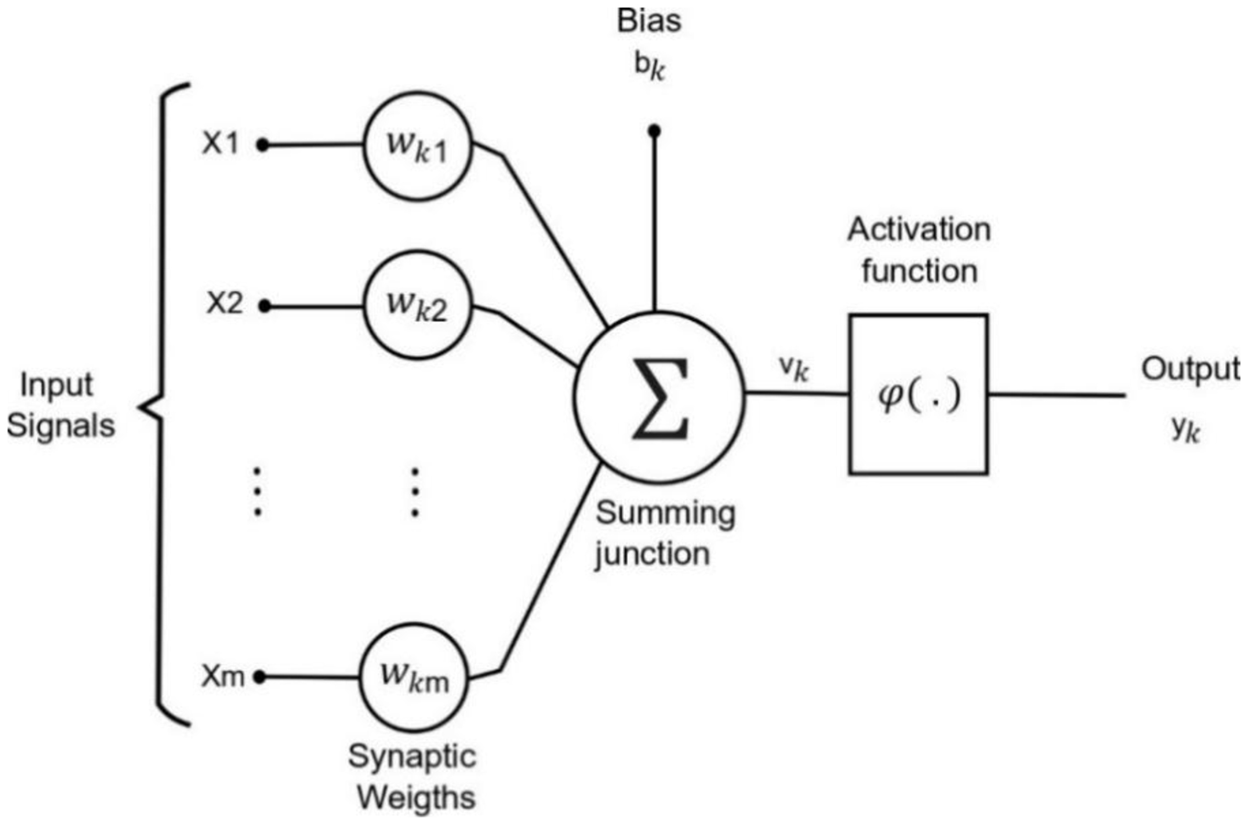
According to Haykin (2001), the artificial neuron model consists of three main components that operate sequentially and interdependently (Figure 1):

Figure 1
Graphical Representation of an Artificial Neuron (adapted from Haykin, 2001).

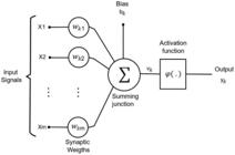
a) Set of synapses: synapses connect the neuron to other neurons or external inputs and are characterized by a synaptic weight $w_i$​. This weight determines the strength and polarity of the connection, influencing the magnitude and direction of the input signal. Weights can amplify ($w_i>1)$, attenuate $(0<w_i<1)$, or invert $\left(w_i<0\right)$ input signals. Each input's contribution to the neuron is determined by multiplying the input signal $x_i$ by its corresponding weight $w_i$.

b) Summation junction: the summation unit performs a weighted sum of the input signals, expressed by the following Equation 1:

$u_k={\displaystyle \sum }_{j=1}^m{w}_{kj}.x_j$ (1)

Where$w_k={\left[w_{k1},w_{k2},\dots ,w_{km}\right]}^T\text{is the weight vector and}x={\left[x_1,x_2,\dots ,x_m\right]}^T$ is the input vector. This weighted sum can be compactly written as Equation 2:

$u_k=w_k^{T}x$ (2)

Here, $w_k^T$ represents the dot product between the weight vector and the input vector. The variable $x={\left[x_1,x_2,\dots ,x_m\right]}^T$ corresponds to the projection of the vector $x$ in the direction of the weights $w_k$in the vector space ${ℝ}^m$.

c) Activation function: The activation function is crucial for introducing non-linearities into the model. It plays a vital role in enabling the network to extract and represent complex, non-trivial patterns from input data, as emphasized by Haykin (2001). Below, some of the most commonly used activation functions and their key characteristics are explored.

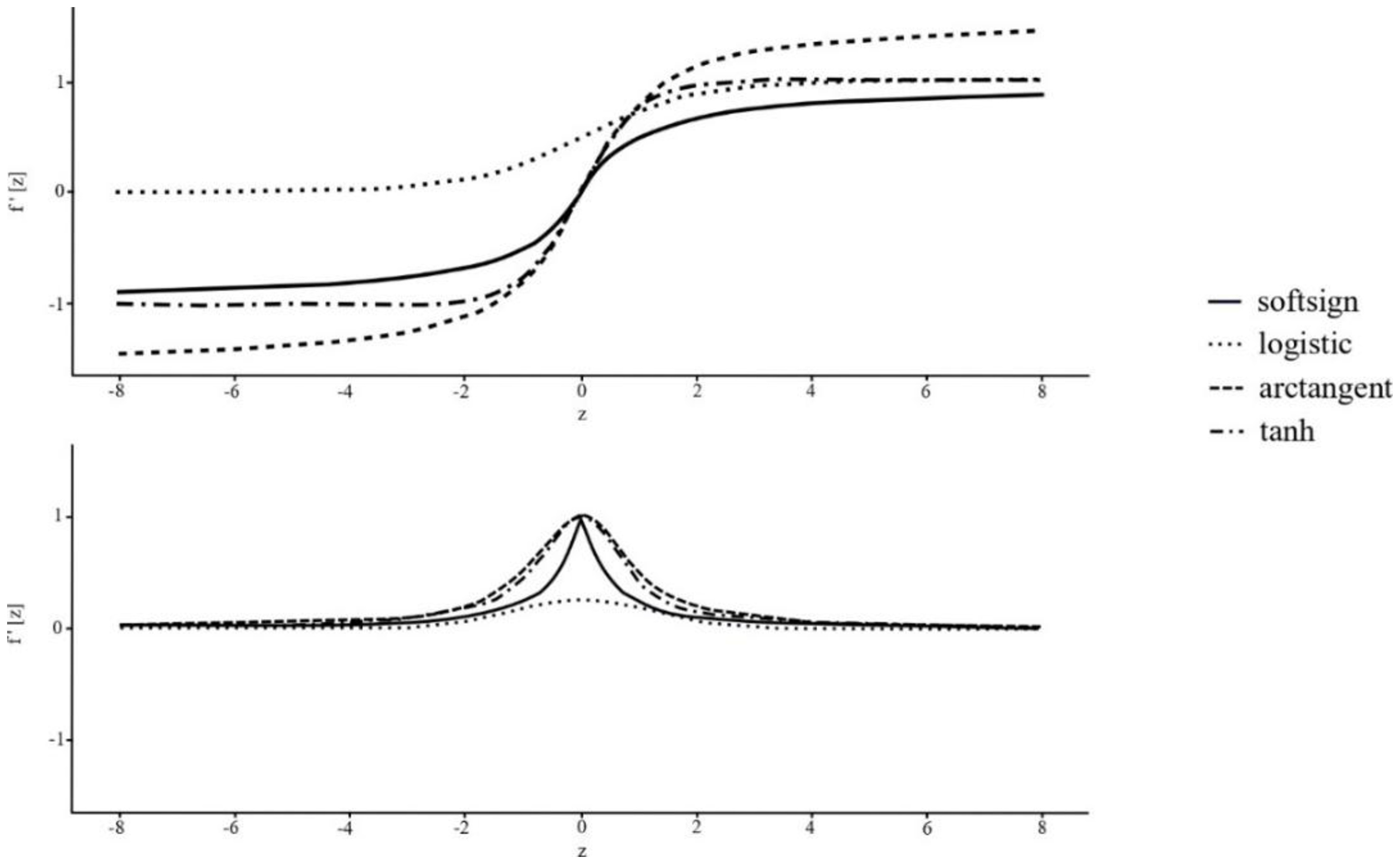
The sigmoid function (Figure 2) is a differentiable, bounded mathematical function that maps input values to a specific range, such as (0, 1) or (-1, 1). This property makes it particularly well-suited for binary classification tasks (Lederer, 2021). Its characteristic S-shaped curve ensures smoothness and continuity, which simplifies the optimization of network parameters using gradient-based methods. The hyperbolic tangent, a type of sigmoid function, is denoted by and is defined by Equation 3.

Figure 2
Sigmoid activation functions used in artificial neurons (adapted from Lederer, 2021).

$f_{tanh}\left(z\right)=\frac{e^z-e^{-z}}{e^z+e^{-z}}$ (3)

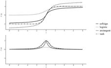
Despite its strengths, the sigmoid function faces the issue of vanishing gradients when applied to deep neural networks (Glorot et al., 2011; Lederer, 2021). This problem arises because the sigmoid's derivatives become very small for extreme input values - whether positive or negative - leading to gradients that are nearly zero. As a result, the network struggles to train and update its weights efficiently (Lederer, 2021).

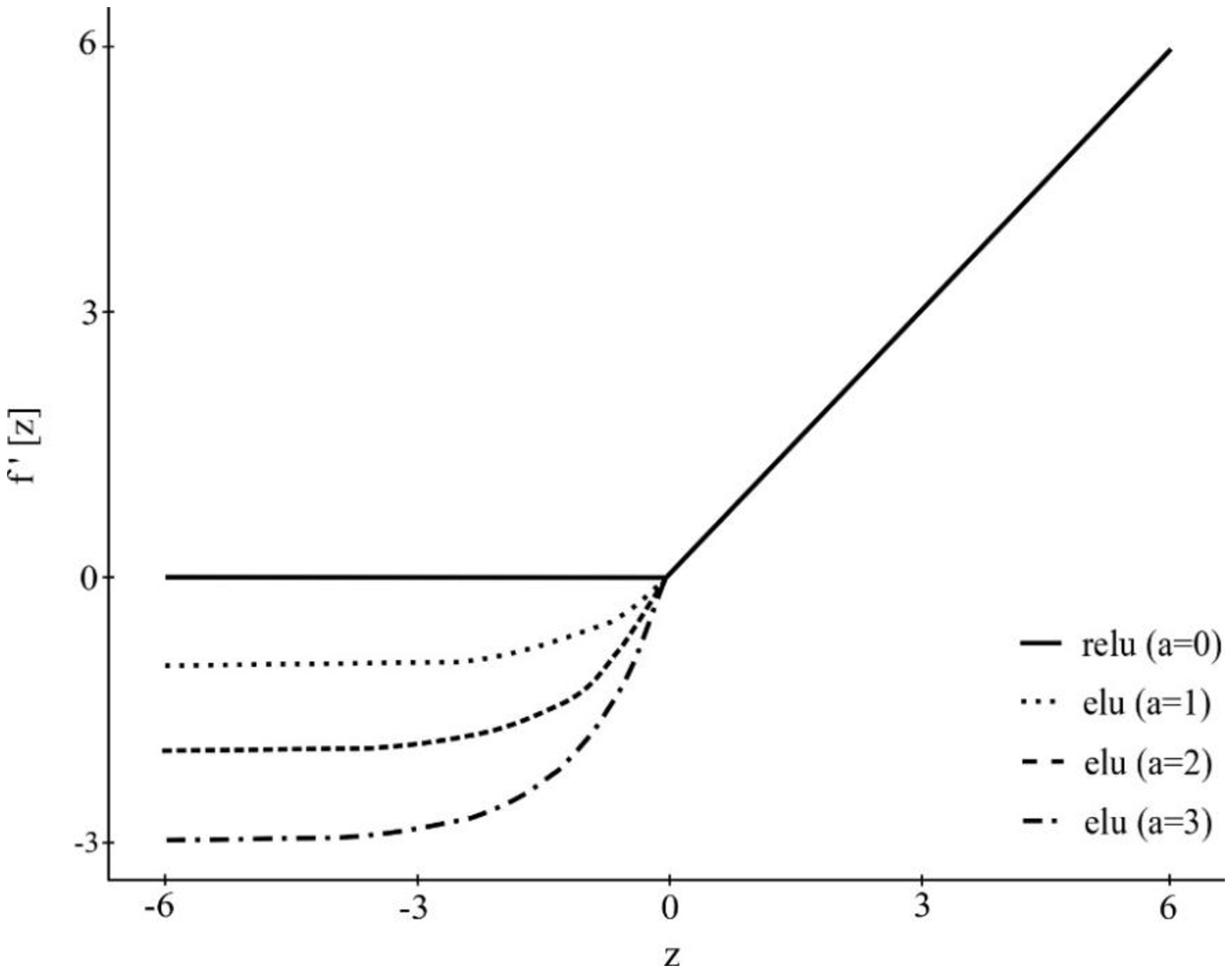
Piecewise linear activation functions (Figure 3), such as ReLU (Rectified Linear Unit) and its variants, are composed of linear segments, offering greater computational efficiency than functions that rely on more complex operations, such as exponential functions. ReLU is defined in Equation 4.

Figure 3
Piecewise linear activation functions in artificial neurons (adapted from Lederer, 2021).

$ReLU\left(x\right)=\text{max}\left(\mathrm{0,}x\right)$ (4)

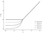
The ReLU function is widely adopted in deep neural networks due to its computational simplicity and the fact that it maintains a non-zero derivative for x>0, which helps mitigate the vanishing gradients problem (Lederer, 2021). However, it has a limitation: it can produce 'dead neurons' when the input is negative. In such cases, the output of ReLU remains consistently zero, preventing weight updates during training. This phenomenon can hinder the learning process, mainly when a significant proportion of inputs result in negative values, making it difficult for the network to adapt to the data's features (Lederer, 2021).

Training artificial neural networks

Training neural networks is an iterative and essential process for optimizing model performance by adjusting its internal parameters, known as weights. The network's parameter vector consists of multiple elements, fine-tuning weights during each training iteration. The structure and values of these parameters vary depending on the number of layers and neurons in the network, reflecting the model's specific architecture and complexity. Proper definition and selection of these parameters are critical to ensuring efficient learning and strong generalization capabilities, as they determine how signals propagate and are processed across the different layers (Hastie, 2009).

The cost function, the error function, is a key metric that quantifies the discrepancy between the model's predictions and observed values. This function plays a vital role in the training process, guiding the necessary adjustments to the model's parameters to improve predictions. In regression problems, the most commonly used error function is the Mean Squared Error (MSE), which corresponds to the sum of squared errors normalized by the number of samples (Haykin, 2001; Hastie, 2009). The MSE can be mathematically represented by Equation 5.

$E_n=\frac{1}{n}{\displaystyle \sum }_{j=1}^m{\left(y_j-{\widehat{y}}_j\right)}^2$ (5)

The cost function$E_n$​ is represented as the function that is aimed to be minimized through parameter optimization. Here,$m$is the total number of examples in the dataset; $y_j$is the actual (observed) value for the i-th example in the dataset;${\widehat{y}}_j$​ is the model's predicted value for the ii-th example; and${\left(y_j-{\widehat{y}}_j\right)}^2$is the squared error for each example.

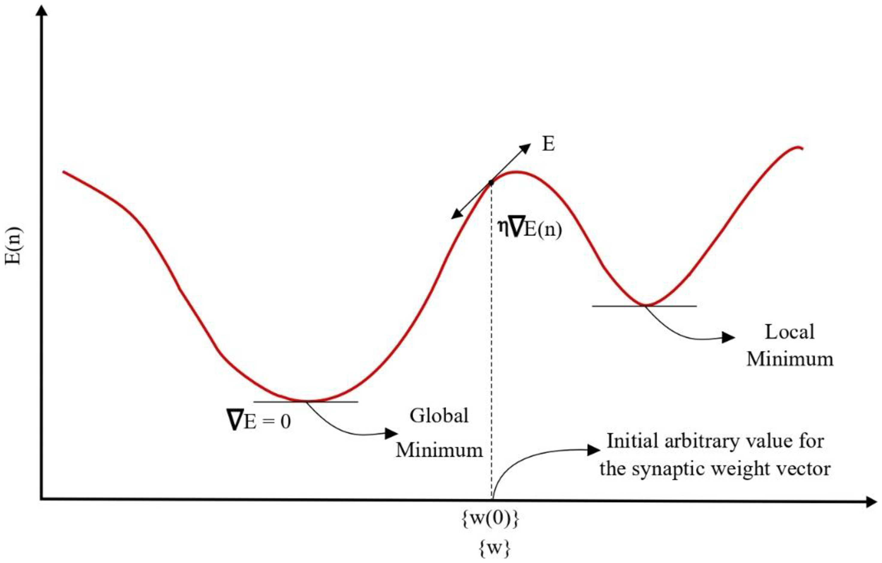
In neural networks, the error function is typically minimized using the backpropagation algorithm, which relies on the iterative nature of the gradient descent (Figure 4). This algorithm is a continuous process, consisting of two key steps that are crucial for adjusting the network's weights (Rumelhart et al., 1986; Haykin, 2001; Hastie, 2009).

Figure 4
Visualization of the cost function minimization.

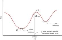
The forward pass is the phase where input data is passed sequentially through a neural network's layers, starting from the input layer and ending at the output layer. During this process, the activations of neurons in each layer are computed based on the current weights and the defined activation functions. The main objective of this step is to generate the network's predicted outputs, which are then compared to the actual values when calculating the cost function. This comparison allows for an assessment of the model's performance.

The backward pass, a critical step, begins with calculating the error, which is the difference between the network's predictions and the actual values. This error is then propagated backward through the network's layers, starting at the output layer and moving toward the input layer. During this phase, the gradients of the error concerning the network's weights are calculated using the backpropagation algorithm. These gradients play a pivotal role in adjusting the weights to reduce the difference between the network's predictions and the actual values, thereby improving the model's accuracy (Rumelhart et al., 1986).

The update of the weights in each iteration$n+1$is given by Equation 6.

$w_{km}\left(n+1\right)=w_{km}\left(n\right)-\eta \frac{\partial E}{\partial w_{km}}$ (6)

Here$w_{km}\left(n\right)$represents the weight between neuron m in layer k at iteration n; η is the learning rate at iteration n, which controls the magnitude of the weight updates; and$\frac{\partial E}{\partial w_{km}}$​ is the gradient of the cost function, measuring the sensitivity of the error E concerning the weight$w_{km}$.

Gradient descent is one of the most fundamental optimization techniques in training neural networks. Its core principle revolves around iteratively updating the network's parameters (weights) in the direction opposite to the gradient of the cost function, thereby progressively minimizing its value. While the algorithm is conceptually straightforward, it can become computationally demanding, particularly in deep neural networks or when dealing with many parameters. This is because calculating each sample's gradient requires substantial computational resources. Furthermore, the performance of gradient descent highly depends on the choice of the learning rate. Poorly selected learning rates can lead to slow convergence, stagnation, or even divergence, underscoring the importance of carefully tuning this hyperparameter to ensure the efficiency and effectiveness of the training process (Haykin, 2001; Hastie, 2009).

The LBFGS (Limited-memory Broyden–Fletcher–Goldfarb–Shanno) algorithm, introduced by Nocedal (1980), represents a more advanced gradient-based optimization technique, renowned for its efficiency in handling problems involving a large number of parameters. As a member of the quasi-Newton family of methods, LBFGS leverages approximations of the inverse Hessian matrix to accelerate convergence rates. Unlike traditional methods that require storing the entire Hessian matrix, LBFGS adopts a limited-memory approach, retaining only information about gradients and previous iterations. This strategy significantly reduces memory and computational requirements, making LBFGS particularly well-suited for high-dimensional problems, such as training neural networks with extensive parameter sets (Hastie, 2009; Ali, 2021).

The parameter updates in the LBFGS algorithm are determined by Equation 7.

$w_{n+1}=w_n-\eta .H_n^{-1}.\nabla E\left(w_n\right)$ (7)

Here,$H_n^{-1}$denotes the inverse approximation of the Hessian matrix, and$\nabla E\left(w_n\right)$represents the gradient of the cost function with respect to the weights.

The Adam (Adaptive Moment Estimation) algorithm is another widely adopted optimization method that integrates the strengths of stochastic gradient descent with techniques based on first- and second-order moments. Adam dynamically adjusts the learning rate for each model parameter by leveraging exponentially decaying averages of the gradient's mean and variance. Renowned for its computational efficiency, rapid convergence, and numerical stability, Adam has become a popular choice for optimizing deep neural networks and other large-scale applications (Kingma & Ba, 2015).

Cross validation

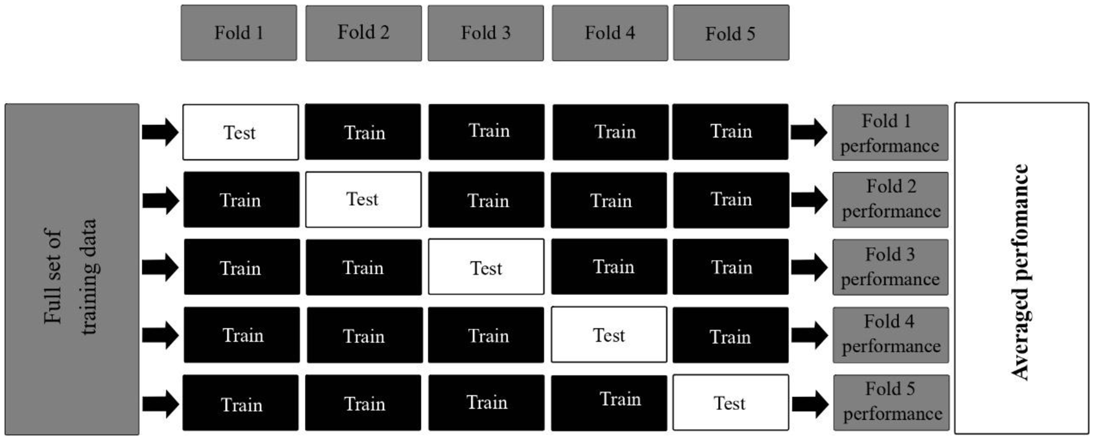
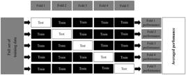
Cross-validation is a key technique for assessing the generalization ability of machine learning models, mainly when working with limited datasets. Unlike a simple train-test split, this method offers a more reliable estimate of model performance by minimizing variations that arise from arbitrary data splits. The process involves systematically dividing the original dataset into multiple subsets or folds. The model is then iteratively trained on a portion of the data and tested on the remaining portion. This approach ensures that every data point is used for training and testing across different iterations, reducing the impact of statistical biases and providing a more accurate evaluation of the model's predictive power (Kohavi, 1995).

Cross-validation begins by systematically splitting the dataset into kk subsets, known as folds, typically of equal size (Figure 5). Each fold represents a distinct subset of the data, allowing every observation to serve for training and validation across the iterations. During the iterative training and testing process, the model trains on k−1k−1 folds, while the remaining fold serves exclusively for validation. The algorithm repeats this process kk times, ensuring that the model evaluates each fold exactly once as the test set. This iterative approach minimizes the influence of specific data splits on the results, reducing statistical variability and improving model performance.

Figure 5
Performance evaluation through cross-validation (adapted from Iacomcafé, 2025).

MATERIALS AND METHODS

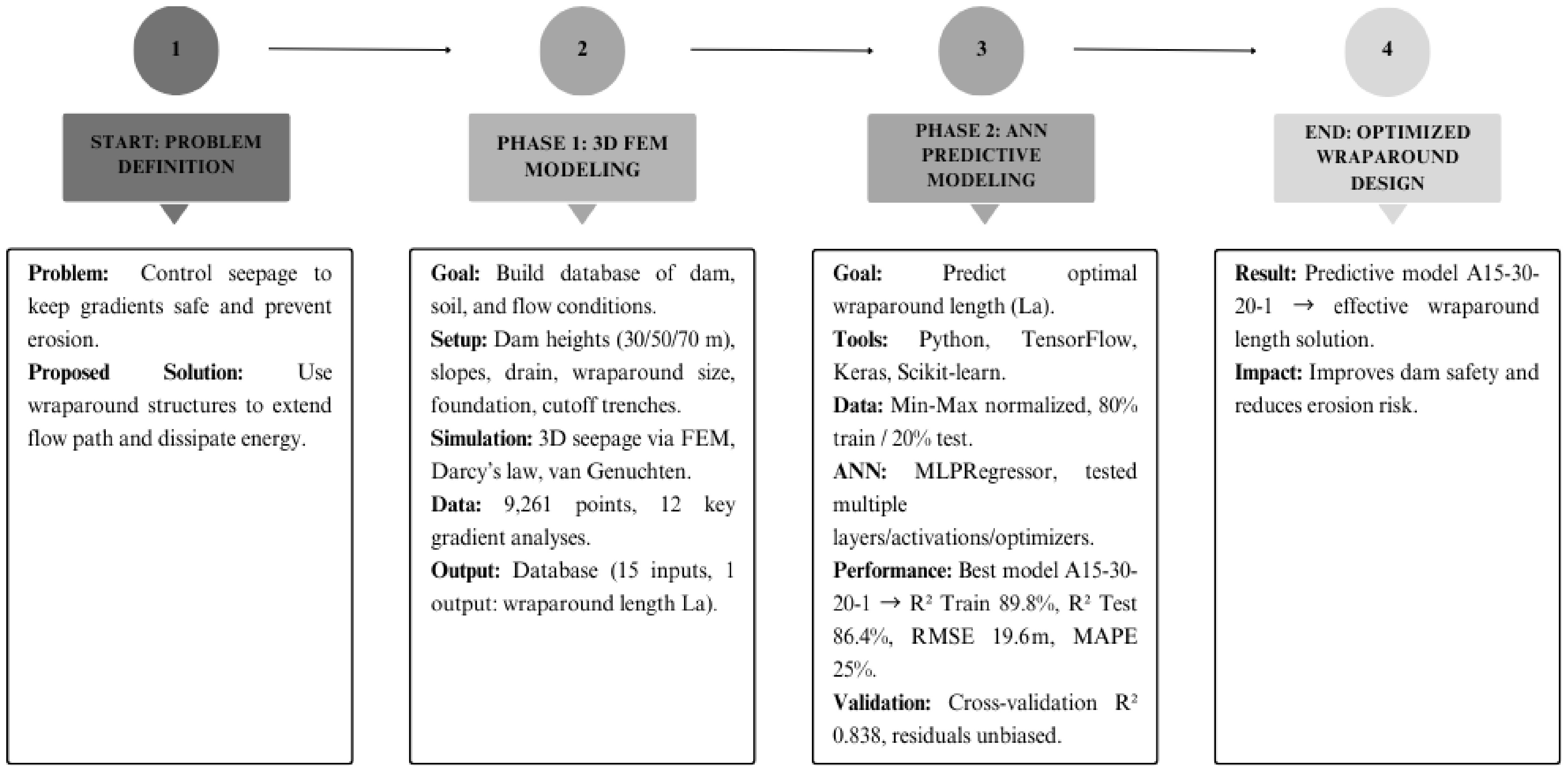
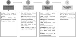
The development of the predictive model followed a structured approach in two integrated and complementary stages: three-dimensional computational modeling and the implementation of a predictive model using a multilayer perceptron (MLP) artificial neural network (ANN). The first stage involved running 3D simulations to build a comprehensive database covering various geometric, geotechnical, and hydrological conditions. This allowed for a thorough assessment of the key factors affecting system performance. The data collected served as the foundation for training a neural model designed to estimate the optimal length of the wraparound. The overall procedure is summarized in the FEM-ANN Integrated Workflow presented in Figure 6.

Figure 6
FEM-ANN Integrated Workflow.

Building the database from 3D numerical flow simulations in earth dams

A control structure known as a wraparound is implemented to mitigate the risks associated with uncontrolled internal seepage, particularly internal erosion. This structural feature, designed as an extension of the spillway's concrete wall, increases the effective seepage path, promoting the gradual dissipation of hydraulic energy. By reducing hydraulic gradients along the soil-structure interface, the wraparound helps prevent erosion-related instability and ensures the dam's structural integrity.

The introduction of the wraparound transforms the seepage problem from a two-dimensional flow scenario into a fully three-dimensional one. Its presence alters the velocity distribution of the percolating water, introducing components in all three spatial directions. Because of this, accurately capturing the flow behavior at the soil-structure interface requires 3D numerical simulations. The wraparound makes the seepage path more complex, increasing the interaction between the soil and concrete and causing the flow to traverse multiple planes and directions before reaching the downstream slope. This redirection of flow energy helps dissipate hydraulic forces and reduces localized gradients at the critical interface, ultimately enhancing the structure's stability.

Mathematically, three-dimensional flow through porous media is governed by the generalized Darcy equation, as expressed in Equation 8.

$\frac{\partial }{\partial x}\left(k_x\frac{\partial h}{\partial x}\right)+\frac{\partial }{\partial y}\left(k_y\frac{\partial h}{\partial y}\right)+\frac{\partial }{\partial z}\left(k_z\frac{\partial h}{\partial z}\right)=S_s\frac{\partial h}{\partial t}$ (8)

In this equation, $h\left(x,y,z,t\right)$ represents the hydraulic head (in meters), which corresponds to the potential energy of water within the porous medium. The terms $k_x$ , $k_y$, and $k_z$ ​denote the hydraulic conductivity (in m/s) along the $x$, $y$, and $z$ directions, respectively, and can vary depending on the material’s anisotropy. The parameter $S_s$is the specific storage (in $m^{-1}$), which defines the medium’s capacity to store or release water, while $t$ represents time in seconds.

This equation is solved numerically using the Finite Element Method (FEM) within the modeling software, allowing for a detailed analysis of the interaction between the soil and the wraparound structure. By altering the flow dynamics, the wraparound helps dissipate hydraulic forces and reduces localized gradients at the critical interface, ultimately contributing to the dam’s structural stability.

Analyzed parameters

This study focused on evaluating seepage conditions at the soil-structure interface of dams, with particular emphasis on the effectiveness of the wraparound element. Three dam geometries were considered, with heights of 30 m, 50 m, and 70 m, representing different project scales. A set of geometric, geotechnical, and hydraulic parameters was defined for each configuration to capture a wide range of factors influencing hydraulic gradient reduction at the soil-structure interface and its interaction with the wraparound.

Through three-dimensional numerical simulations, 9,261 raw data points were generated, covering a broad spectrum of geometric configurations and hydraulic conditions. Table 1 summarizes these observations and details the variables considered in each scenario. The geometric variations included crest width, slope inclination, and the presence of reinforcement elements such as riprap and drainage systems. The wraparound was parameterized based on its width and length, enabling an assessment of its effectiveness in seepage control, particularly in redistributing hydraulic gradients.

Table 1
Design parameter analysis for wraparound structure evaluation.

Parameter	30m high and 200m long dam	50m high and 333m long dam	70m high and 467m long dam
Crest width	6, 10, 14, 18, 22 meters	10, 22, 36 meters	14, 31, 50 meters
Slope inclination	1:1, 1:2, 1:2.5, 1:3	1:1, 1:2, 1:2.5, 1:3	1:1, 1:2, 1:2.5, 1:3
Riprap width	10, 15, 20, 25, 30 meters	17, 25, 33 meters	24, 35, 46 meters
Drainage blanket with riprap	15, 20, 25, 30, 35, 40 meters	25, 33, 42 meters	35, 46, 59 meters
Foundations	Permeable substrate, 25m thick. Cutoff depth: 5, 8, and 10 meters	Permeable substrate, 42m thick. Cutoff depth: 8, 13, and 17 meters	Permeable substrate, 59m thick. Cutoff depth: 11, 18, and 24 meters
Wraparound length	10, 30, 50, 70, 90 meters	50, 100, 117 meters	70, 140, 187 meters
Wraparound width	1, 2, 3 meters	1.67, 3.33, 5 meters	2.34, 4.66, 7 meters

The dam foundations were modeled with substrates of varying depths and permeability coefficients, allowing for a detailed analysis of how geotechnical conditions and treatment interventions affect subsurface flow behavior. A cutoff wall was incorporated as one of the control measures, with its depth adjusted according to the dam’s characteristics.

The adopted parameterization generated a comprehensive set of computational scenarios, facilitating an in-depth evaluation of how each variable influences hydraulic performance and dam stability. The primary goal was to quantify the percentage reduction in hydraulic gradient by comparing scenarios with and without the control device. This approach provided a clear assessment of the wraparound’s effectiveness in mitigating seepage-related risks and offered technical insights for optimizing its design under different geotechnical conditions.

Table 2 lists the final parameters used as input and output variables in the analysis, along with their respective units and descriptions.

Table 2
Parameters and units used in the analysis.

Type	Symbol	Description	Min	Max	Unit
X1	km	Permeability of the embankment soil	8.25 × 10−5	9.50 × 10−9	m/s
X2	H	Height of the dam	30	70	m
X3	im	Upstream slope gradient	1:03	1:01	°
X4	ij	Downstream slope gradient	1:03	1:01	°
X5	Bc	Crest width	4	36	m
X6	zs	Sill elevation	17.33	60.67	m
X7	Wa	Width of the wraparound	1	7	m
X8	Lt	Length of the horizontal drainage blanket	15	59	m
X9	E	Presence of riprap (0 = no, 1 = yes)	0	1	-
X10	kf	Permeability of the foundation	0.001	8.25 × 10−5	m/s
X11	T	Presence of a cutoff trench (0 = no, 1 = yes)	0	1	-
X12	X	X-coordinate	40	432	m
X13	Y	Y-coordinate	0	87	m
X14	Z	Z-coordinate	44	467	m
X15	Rg	Reduction in hydraulic gradient	0	0.98	%
Y1	La	Length of the wraparound	7	210	m

Three-dimensional numerical simulations

The first phase of this study involved a three-dimensional analysis of dams using the Finite Element Method (FEM) to numerically solve the governing equations of hydraulic flow. These simulations were implemented using the software GeoStudio Seep/W 3D (Seequent, 2024). Multiple finite elements mesh was generated, each with varying numbers of elements and nodes, customized to accommodate different geometries and analysis scenarios. Tetrahedral elements were employed to discretize the domain efficiently, particularly in regions with irregular geometries or at the soil–structure interface. A detailed overview of the modeling setup, input parameters, and output variables is provided in Table 3.

Table 3
Summary of FEM model setup, parameters, and outputs.

Parameter / Aspect	Description	Details / Values
Purpose	Build a database for 3D seepage simulation in earth dams; evaluate wraparound effectiveness.	9261 data points generated for ANN training.
Numerical Method	3D flow in porous media.	Finite Element Method (FEM).
Governing Equation	Generalized Darcy’s law.	∂/∂x(kx ∂h/∂x) + ∂/∂y(ky ∂h/∂y) + ∂/∂z(kz ∂h/∂z) = Ss ∂h/∂t.
Software / Model	Hydrological & geotechnical parameters.	RETEC (2009), Van Genuchten (1980): θs, θr, α, n, Ks.
Mesh	Domain discretization.	Tetrahedral elements; multiple meshes with variable nodes/elements.
Boundary Conditions	Reservoir & slopes.	Variable head upstream; zero-flow lateral slopes.
Dam Assumptions	Simplifications.	Homogeneous dam body; soil–structure interface with 10× permeability.
Analysis Points	Locations for gradient assessment.	3 dam sections × 4 points = 12 (focus on downstream interface).
Dam Height (H)	Design scales.	30 m, 50 m, 70 m.
Slope Ratios	Geometric variation.	1:1, 1:2, 1:2.5, 1:3.
Crest Width (Bc)	Geometric variation.	4–36 m (varies with dam height).
Embankment Permeability (km)	Hydraulic property.	8.25×10−5 to 9.50×10−9 m/s.
Foundation Permeability (kf)	Hydraulic property.	0.001 to 8.25×10−5 m/s.
Weir Elevation (zs)	Reservoir level.	17.33–60.67 m.
Wraparound Width (Wa)	Seepage-control element.	1–7 m (scaled by dam height).
Horizontal Drain Length (Lt)	Seepage-control element.	15–59 m (scaled by dam height).
Rockfill (E)	Reinforcement/drainage.	Binary: 0 (no), 1 (yes). Width 10–46 m.
Cutoff Trench (T)	Seepage-control at foundation.	Binary: 0 (no), 1 (yes). Depth 5–24 m.
Coordinates (X,Y,Z)	Analysis point location.	X: 40–432 m; Y: 0–87 m; Z: 44–467 m.
Wraparound Length (La)	Seepage-control dimension.	7–210 m (scaled by dam height).
FEM Output (Rg)	Effectiveness indicator.	Hydraulic gradient reduction: 0–0.98 (used as ANN input).

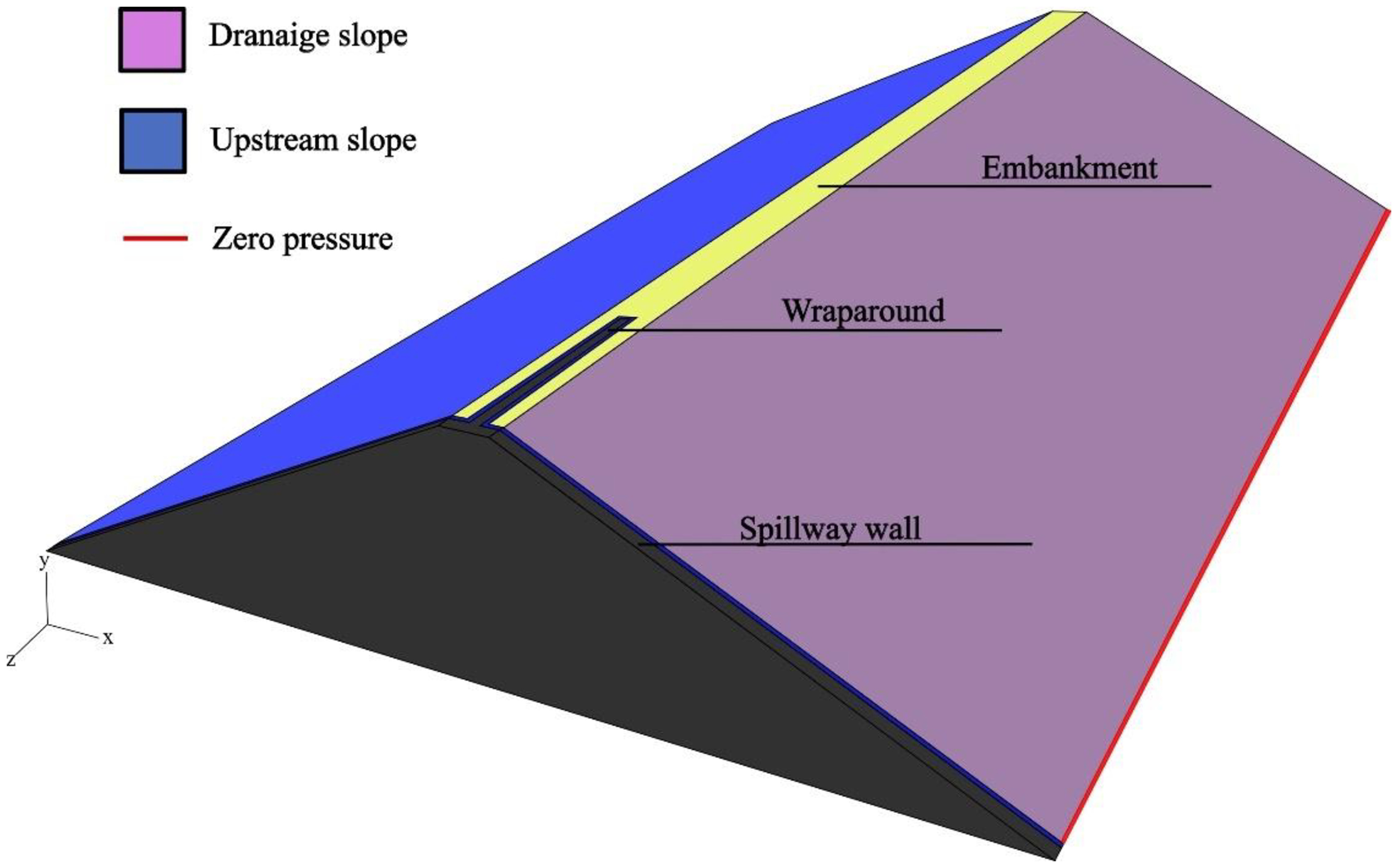
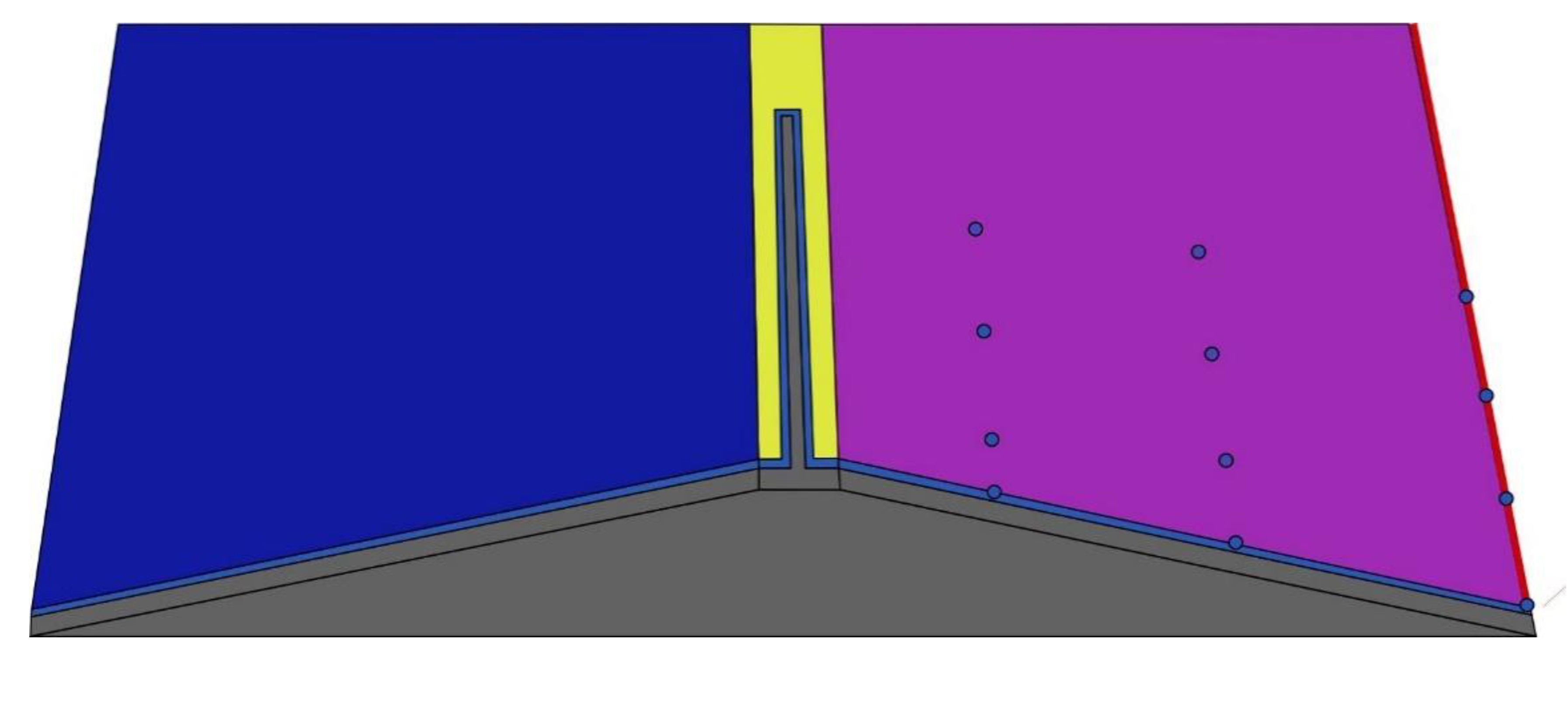
The boundary conditions included an upstream hydraulic head that varied depending on the dam configuration and a zero-flux condition along the slopes, representing impermeable lateral boundaries (Figure 7). This setup ensured an accurate representation of hydraulic behavior and each scenario's unique characteristics.

Figure 7
Three-dimensional model of the dam with representation of the variables involved.

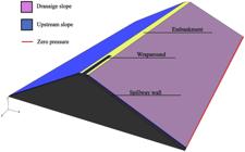
The dam body was assumed to be homogeneous to streamline the modeling process and facilitate the analysis of soil-structure interactions. This simplification eliminated additional complexity caused by soil heterogeneity, allowing for a clearer assessment of the wraparound’s influence on hydraulic performance.

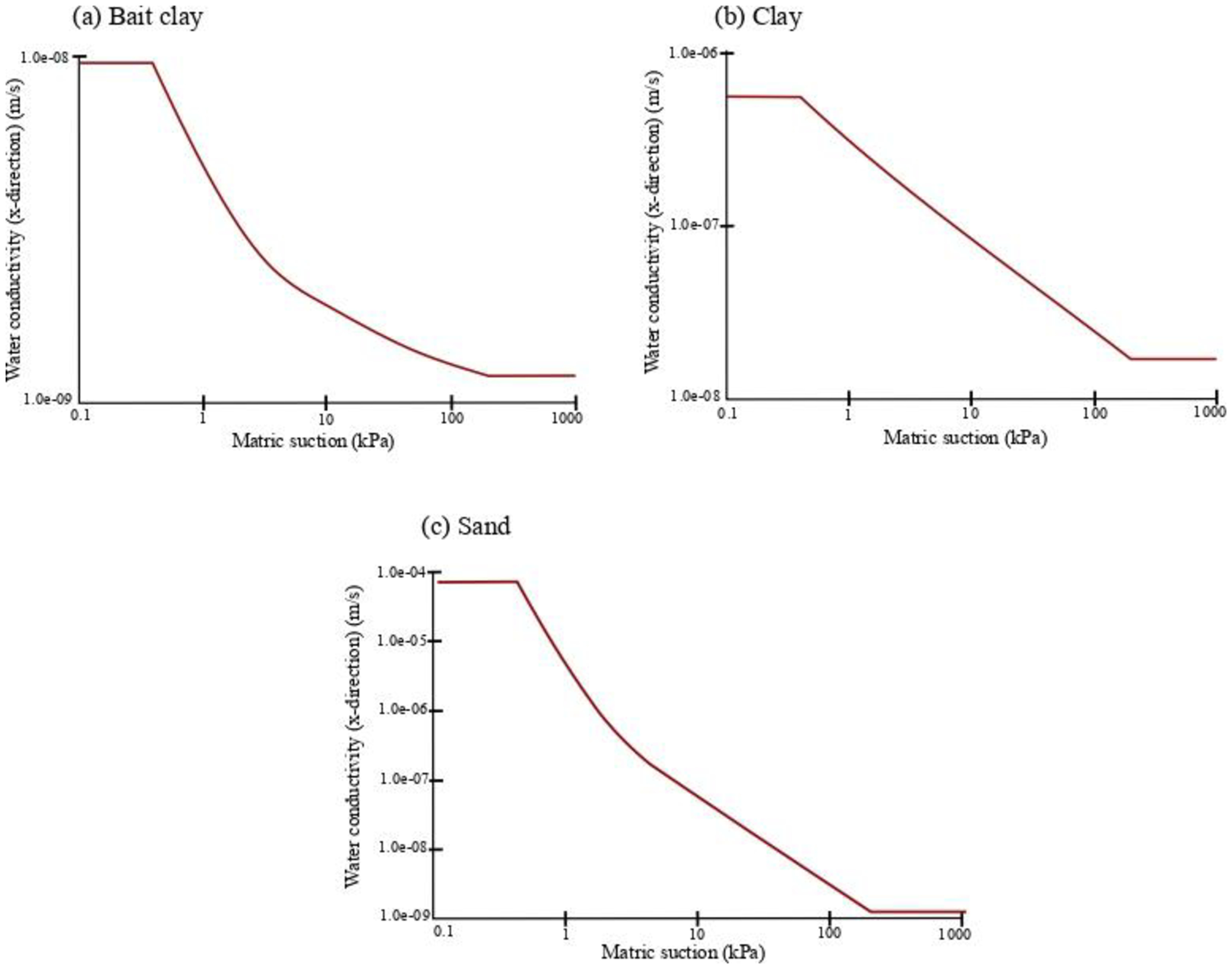
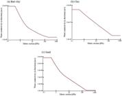
The hydrological and geotechnical parameters for modeling flow in unsaturated porous media were derived from the RETEC software (RETEC, 2009) using the Van Genuchten model (Van Genuchten, 1980). This model requires input parameters such as saturation moisture content (θs), residual moisture content (θr), the α parameter (related to air entry pressure), exponent n (which defines the retention curve shape), and saturated hydraulic conductivity (Ks). These parameters define the relationship between matric suction and moisture content, describing water retention in the soil and governing unsaturated hydraulic conductivity, both essential for accurately modeling seepage in porous media. The hydraulic conductivity functions obtained for the three representative materials, sand, bait clay, and clay, are presented in Figure 8, providing a direct visualization of how the Van Genuchten parameters influence water flow behavior under unsaturated conditions.

Figure 8
hydraulic conductivity functions in the numerical simulations.

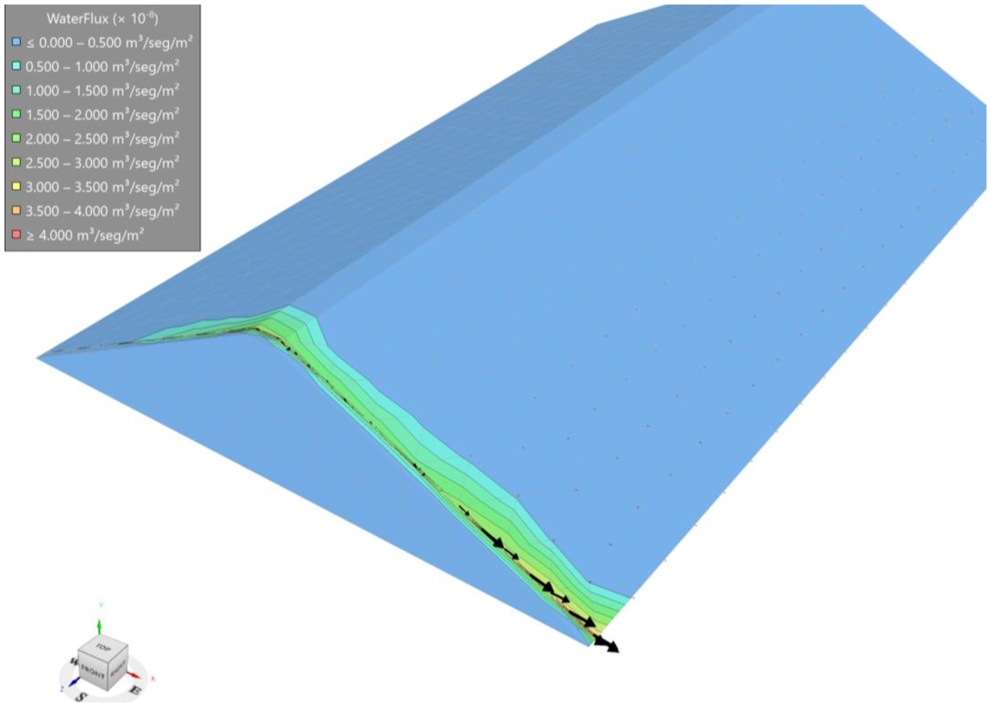
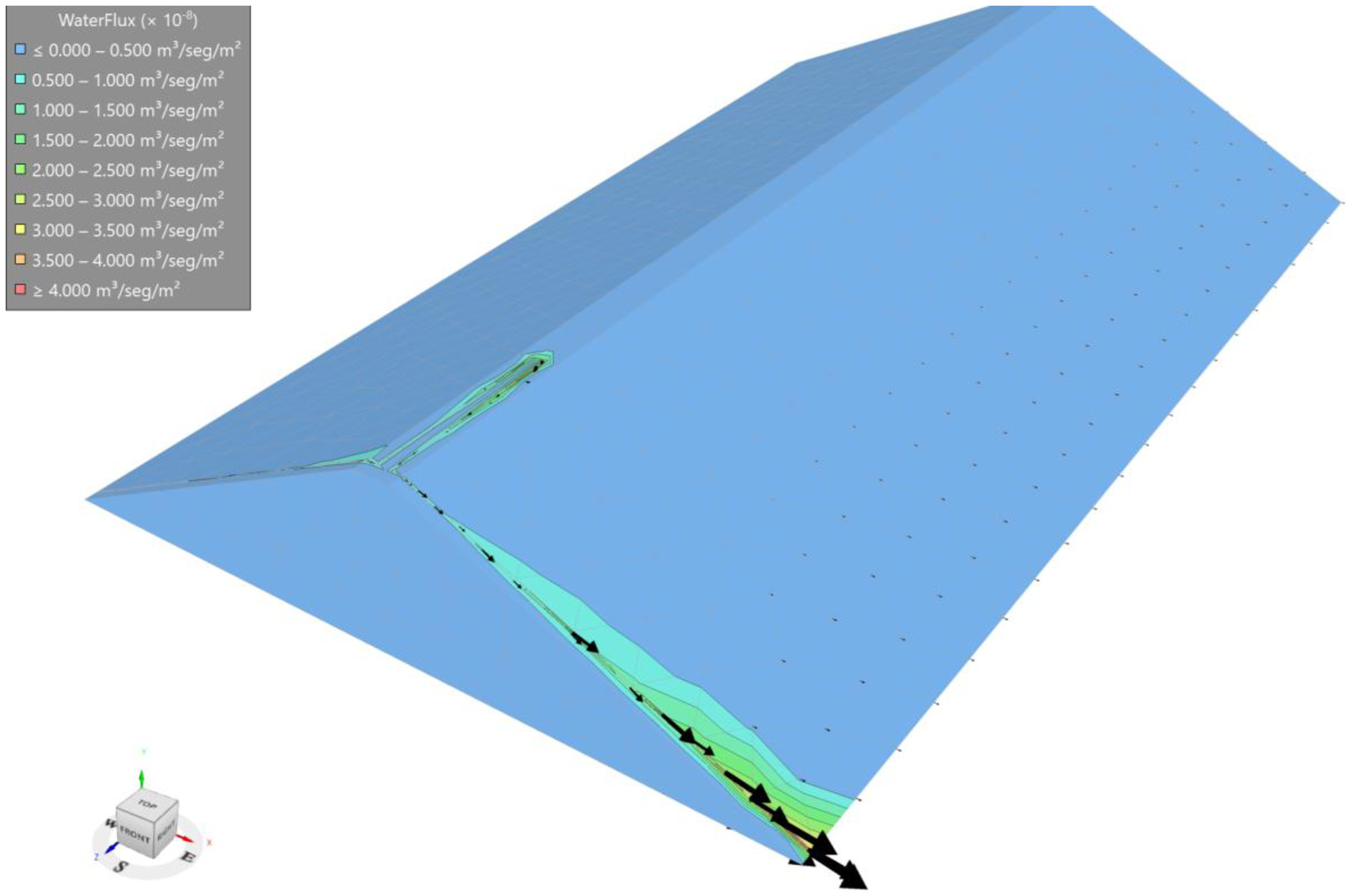
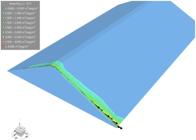
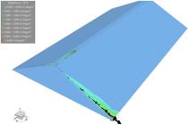
In the numerical simulations, discontinuities at the soil structure interface, such as variations in permeability and hydraulic conductivity, were represented by a thin layer with permeability ten times higher than that of the main dam body. This modeling strategy allowed a more accurate representation of the distinct hydraulic behavior of the interface and its role in flow redistribution. Figure 9 presents the distribution of flow lines and the discharge through the dam without the wraparound device, while Figure 10 shows the same analysis with the device installed. The comparison highlights the efficiency of the wraparound in reducing seepage discharge and controlling hydraulic gradients. These outcomes provide valuable insights into the influence of discontinuity zones on seepage behavior, reinforcing their relevance to the overall stability and safety of the structure.

Figure 9
Seepage flow without wraparound device.

Figure 10
Seepage flow with wraparound device.

Analysis of hydraulic gradients

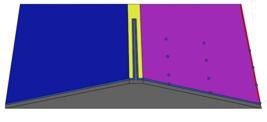
The methodology adopted in this study focused on selecting three key locations along the dam, with four specific analysis points within each of these strategic regions. The primary objective was to characterize and quantify hydraulic gradients by comparing the dam’s original configuration with a modified version that included the seepage control device. This comparison aimed to assess the device’s effectiveness in reducing hydraulic gradients and to support its optimal design.

The selection of analysis locations, illustrated in Figure 11, followed a systematic approach based on identifying critical seepage zones at the soil-structure interface. The analysis points were strategically positioned to evaluate the areas adjacent to the interface, where the wraparound directly influences hydraulic gradient mitigation, and the regions closer to the device. Particular attention was given to points near the downstream section of the dam, as this area is more susceptible to high hydraulic gradients and concentrated hydraulic forces, as highlighted by Sousa (2013).

Figure 11
Points analyzed in the flow analyses.

Development of the prediction model using artificial neural networks

The second phase of the study involved applying Artificial Neural Networks (ANNs), specifically Multilayer Perceptrons (MLPs), to establish a mathematical function that correlates the input variables listed in Table 2 with the output variable$La\text{}$, which represents the optimal length of the seepage control device.

Mathematically, the ANN can be expressed by Equation 9:

$L_a=f\left(X;\theta \right)$ (9)

WhereXis the input vector composed of the 15 variables described in Table 2, and θ represents the network's parameters, including the weights W and biases b, which are adjusted during the training process.

The ANN learns the function $f\left(X;\theta \right)$ through successive nonlinear transformations applied at each hidden layer. Formally, the process of information propagation through the network can be described as follows:

$X^1=\sigma \left(W_{1}X+b_1\right)$ (10)

$X^2=\sigma \left(W_2{X}^1+b_2\right)$ (11)

$L_a=W_n{X}^{n-1}+b_n$ (12)

Where$X^i$ represents the activations of the i-th layer of the network,$\sigma$(.) is the activation function, and$W_i$​ and$b_i$ are the weight matrix and bias vector associated with the i-th layer, respectively.

The implementation of the ANN is presented in Appendix A – Code for Training and Evaluating Different Artificial Neural Network Configurations. The implementation of the ANN was carried out using the Python programming language, supported by specialized machine learning libraries such as TensorFlow, Keras, and Scikit-learn (Géron, 2022). These tools enabled the efficient construction, training, and validation of the model, ensuring the optimization of hyperparameters and the evaluation of the network's performance.

The application of ANNs facilitated the identification of complex, nonlinear patterns within the data and provided an optimized solution to the problem at hand. The adaptive nature of these networks, which autonomously adjust their synaptic parameters based on input data and simulated scenarios, was crucial for determining the optimal length$La\text{}$of the control device. This approach ensured the minimization of the hydraulic gradient, resulting in enhanced performance of the seepage control system and improved operational efficiency of the device.

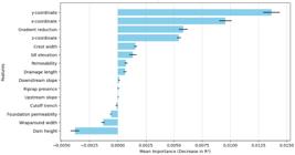
Model interpretability analysis via permutation importance

In this study, it is particularly relevant to quantify the influence of each input variable on the prediction of the output variable, namely the wraparound length (La). Understanding feature importance not only enhances the interpretability of the model but also provides insights into the underlying physical or geotechnical mechanisms that govern the phenomenon being modeled.

To achieve this, we employed permutation importance, a model-agnostic approach that evaluates the contribution of each feature to the overall predictive performance. The method works by randomly shuffling the values of a given feature and measuring the resulting decrease in model accuracy. If the disruption of a feature leads to a substantial drop in performance, this feature is considered highly influential.

The coefficient of determination (R²) was used as the performance metric. The decrease in R² observed after the permutation indicates the relative importance of the feature: the larger the reduction, the more critical the feature is for accurate predictions. This procedure allowed us to rank the variables according to their impact on the predictive capability of the model, offering a clear and quantitative assessment of their relevance.

Data normalization and splitting

Data normalization is critical in preparing datasets for training machine learning models, ensuring that all independent variables are processed on compatible scales. This procedure involves rescaling the values of variables to predefined ranges, such as [0, 1] or [-1, 1], to preserve the relative relationships between data points and prevent variables with larger magnitudes from dominating the model. While normalization does not eliminate the influence of outliers, it plays a vital role in standardizing variable scales and reducing numerical discrepancies that could compromise training stability and model convergence (IPNET, 2023).

Among the various normalization techniques, one of the most widely used is Min-Max Scaling. This method adjusts the values of variables to a predefined range, typically [0, 1], ensuring that all features are proportionally scaled. The transformation is performed using the following mathematical expression:

$X_{norm}=\frac{X-X_{min}}{X_{max}-X_{min}}$ (13)

Where$X$represents the original value of the variable,$X_{min}$​ is the minimum observed value of the variable in the dataset, and$X_{max}$​ is the maximum observed value of the variable in the dataset. This transformation ensures that all values are mapped within the specified range, preserving the relative distribution of the data and maintaining the relationship between the original values.

Data normalization was performed using the Min-Max Scaling method, implemented via the MinMaxScaler class from the scikit-learn library. The scaler was fitted to the training set to calculate the normalization parameters and then uniformly applied to both the training and test sets, ensuring consistency in the scaling of the input and output variables.

The dataset used in this study comprised a total of 9261 raw data points, originally generated from three-dimensional numerical simulations of flow in earth dams. After preprocessing, which involved the removal of missing values using the dropna() function, the effective dataset employed for training the machine learning algorithms was reduced to 1658 entries. For the Artificial Neural Network (ANN) models, the dataset was partitioned into 80% for training (approximately 1326 samples) and 20% for testing/validation (approximately 332 samples), ensuring a consistent and reliable basis for model development and performance evaluation.

Hyperparameters of the neural model

The predictive framework adopted in this study is based on Artificial Neural Networks (ANNs) of the Multilayer Perceptron (MLP) type, implemented through the MLPRegressor module from the scikit-learn library (Pedregosa et al., 2011). MLPs are feedforward neural networks capable of modeling complex nonlinear relationships by iteratively adjusting synaptic weights and biases through optimization algorithms.

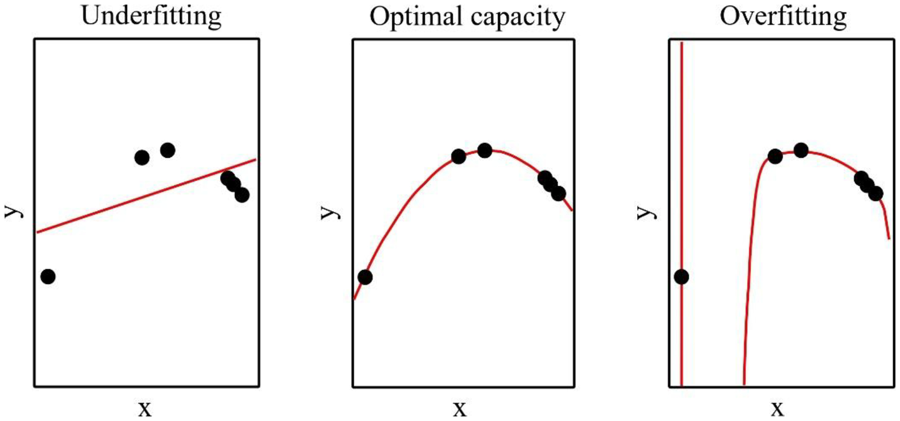
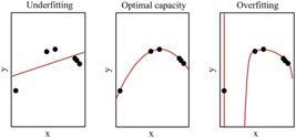
D Defining the architecture of a neural network is a critical step, since inappropriate design choices can result in underfitting, when the model fails to capture the underlying data complexity, or in overfitting, when it loses its ability to generalize (Figure 12). As emphasized by Goodfellow et al. (2016), structural tuning is essential to balance learning efficiency and predictive accuracy. The determination of an optimal architecture, including the number of hidden layers and neurons, is therefore fundamental to model performance. Studies have shown that an excessive increase in adjustable parameters, or hyperparameters, does not necessarily lead to higher accuracy and may instead cause overfitting. In many cases, architectures with fewer hidden layers can achieve better generalization, depending on the complexity of the hydraulic problem being modeled (Souza et al., 2021).

Figure 12
Underfitting and Overfitting (adapted from Goodfellow et al., 2016).

The hyperparameterization process involved systematic testing of activation functions, optimization algorithms, and network architectures:

• Activation functions: Rectified Linear Unit (ReLU), sigmoid, and hyperbolic tangent (tanh).

• Optimization algorithms: Adam (Kingma & Ba, 2015) and LBFGS (Nocedal, 1980).

• Network architectures: Configurations ranged from shallow to deeper topologies, including:

  • A15-100-1 (single hidden layer with 100 neurons),

  • A15-10-10-1, A15-30-20-1, A15-50-50-1, A15-100-50-1,

  • A15-100-100-1 (two hidden layers with 100 neurons each),

  • A15-7-7-7-1 (three hidden layers with seven neurons each).

The dataset was divided into training (80%) and testing/validation (20%) subsets using train_test_split with random_state = 42 to ensure reproducibility. Input (X) and output (y) variables were normalized through Min-Max Scaling, rescaling values to the [0,1] interval to preserve proportionality and enhance training efficiency; the scaler was fitted on the training set and subsequently applied to the testing set.

Each network configuration was trained for a maximum of 2,000 iterations (max_iter = 2000) under a triple-loop procedure combining activation functions, optimization algorithms, and architectures. Performance was then evaluated using standardized metrics to ensure comparability:

• R² (Coefficient of Determination)

• MAE (Mean Absolute Error)

• RMSE (Root Mean Square Error)

• MAPE (Mean Absolute Percentage Error)

This systematic evaluation enabled a detailed assessment of convergence, stability, and predictive accuracy across all tested models.

Analysis of results

During the model performance evaluation phase, a systematic process for selecting and ranking results was adopted, grounded in key quantitative metrics essential for predictive assessment. The metrics used include the Mean Absolute Percentage Error (MAPE), Mean Absolute Error (MAE), Coefficient of Determination (R²), and Root Mean Squared Error (RMSE). The primary objective of this phase was to identify the top three configurations in terms of performance, ensuring a balance between predictive accuracy and computational efficiency. A detailed analysis is presented below.

Initially, the models were ranked in ascending order based on their Mean Absolute Percentage Error (MAPE) values, enabling the identification of configurations with the lowest average percentage deviation between predicted and observed values. MAPE quantifies a model's average error in percentage terms relative to the actual values, providing a scale-independent metric for comparison. The mathematical expression used to calculate MAPE is presented in Equation 14.

$MAPE=\frac{1}{N}{\displaystyle \sum }_{i=1}^N\frac{\left|p_i-r_i\right|}{r_i}$ (14)

Where $p_i$​ represents the predicted values, $r_i$are the observed values, and $N$ is the total number of observations.

The models were then ranked in ascending order based on their Mean Absolute Error (MAE) values, prioritizing configurations with minor average absolute deviations. MAE is the arithmetic mean of the absolute differences between the model predictions ($p_i$​) and the observed values ($r_i$​), assigning equal weight to each error. The mathematical expression for calculating MAE is presented in Equation 15.

$MAE=\frac{1}{N}{\displaystyle \sum }_{i=1}^N\left|p_i-r_i\right|$ (15)

Subsequently, the models were ranked based on their Root Mean Squared Error (RMSE) values. This metric is particularly sensitive to large deviations, penalizing more significant errors more heavily. The mathematical expression for calculating RMSE is given by Equation 16.

$RMSE=\sqrt{\frac{1}{N}{\displaystyle \sum }_{i=1}^N{\left(p_i-r_i\right)}^2}$ (16)

Where $p_i$​ represents the predicted values, $r_i$are the observed values, and N is the total number of observations.

Finally, the models were evaluated based on the Coefficient of Determination ($R^2$) for both training and testing datasets. This analysis prioritized configurations demonstrating consistent predictive performance, ensuring a balance between data fitting and the model’s generalization capability. Its mathematical expression is provided in Equation 17.

$R^2=1-\frac{{{\displaystyle \sum }}_{i=1}^n{\left(r_i-p_i\right)}^2}{{{\displaystyle \sum }}_{i=1}^n{\left(r_i-\overline{r}\right)}^2}$ (17)

Where $r_i$​ are the observed values, $p_i$are the predicted values, $\overline{r}$is the mean of the observed values, and $n$is the total number of observations.

The interpretation of R² ranges from 0 to 1: values close to 1 indicate that the model explains a large portion of the variability in the observed data. In contrast, values near 0 suggest that the model explains little to no variability. Generally, the higher the R², the better the model fits the observed data.

After individually evaluating the models based on each performance metric, an integrated and interpretative analysis of the results was carried out. This approach provided a comprehensive view of each model’s performance, facilitating the selection of the top three configurations for a more detailed analysis.

RESULTS AND DISCUSSION

From the mathematical relationship$La=f\left(X;\theta \right)$, it was possible to identify and quantify the correlations between the wraparound length and the model's input variables. These variables, totaling 15 features, represent the main control parameters of the system under study. The output variable corresponds to the length of the percolation control device (in meters), the quantity predicted by the model.

Training and testing of the evaluated neural models

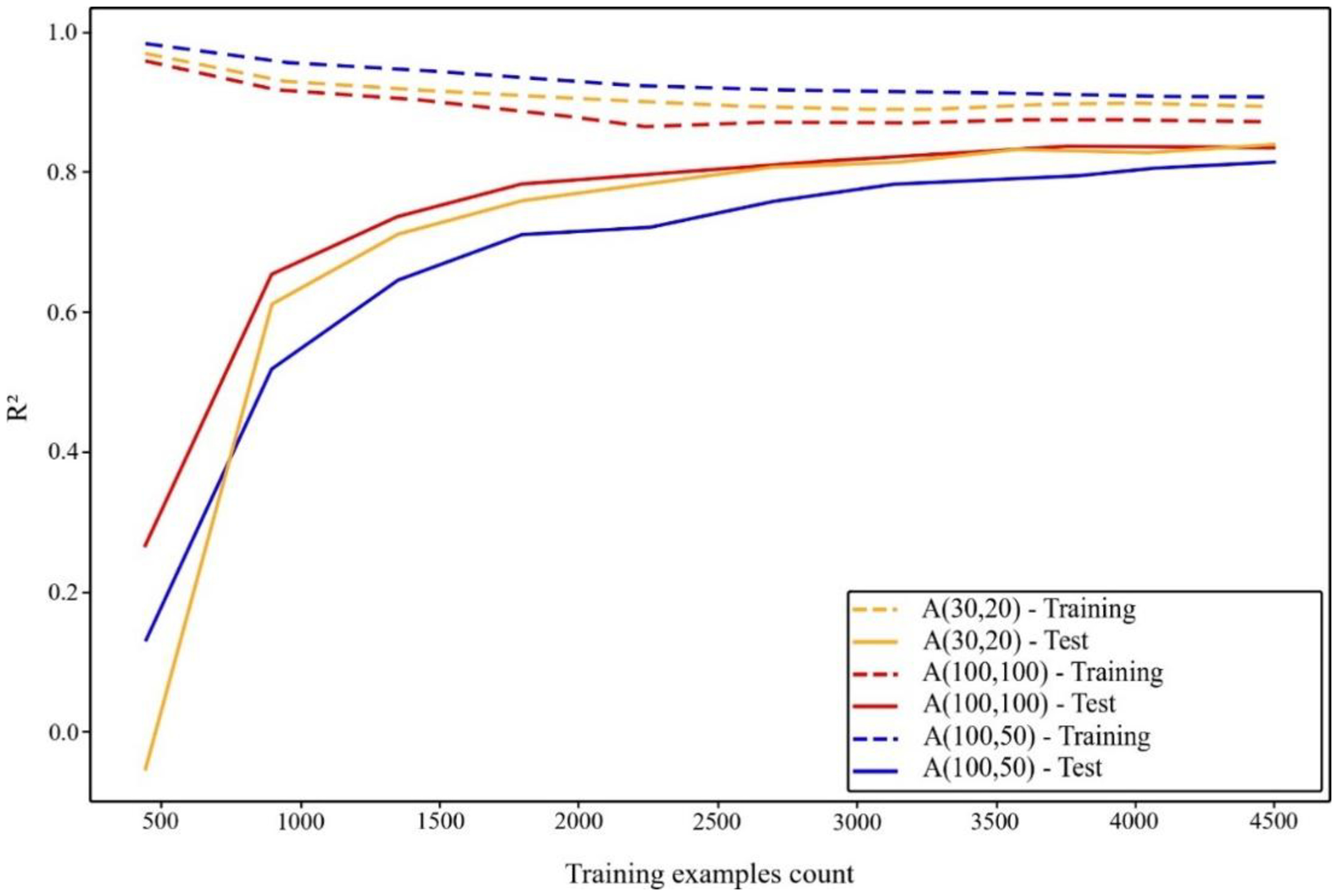
The results from the learning curves (Figure 13) indicate that as the number of training examples increases, all models show continuous performance improvement, reflected in the progressive increase of the coefficient of determination (R²). This behavior suggests that with a larger volume of data, the models can identify more complex patterns and adjust more effectively to the training data. From 3500 examples onward, the performance stabilizes, indicating that the models' generalization capacity reaches a saturation point.

Figure 13
Combined learning curves.

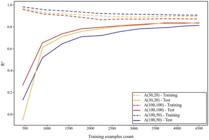
However, the difference between performance on the training and validation sets reveals variations in each model's generalization capability. When this difference is too significant, it suggests that the model may suffer from overfitting, meaning it is excessively tailored to the training data and struggles to predict new data accurately. This behavior indicates that some architectures are more prone to overfitting than others, affecting their reliability in real-world scenarios.

The A15-30-20-1 architecture demonstrated consistent performance across training and validation sets, showing a good generalization ability to new data. This balance suggests that the model successfully captured the underlying patterns in the data without overfitting or losing critical information. In contrast, the A15-100-100-1 architecture exhibited a more pronounced discrepancy between training and validation performance, indicating slight overfitting. While this difference does not render the model unusable, it suggests the need for refining hyperparameters or expanding the training dataset. Finally, the A15-100-50-1 architecture showed the most significant disparity between the two sets, characterizing a potential case of overfitting.

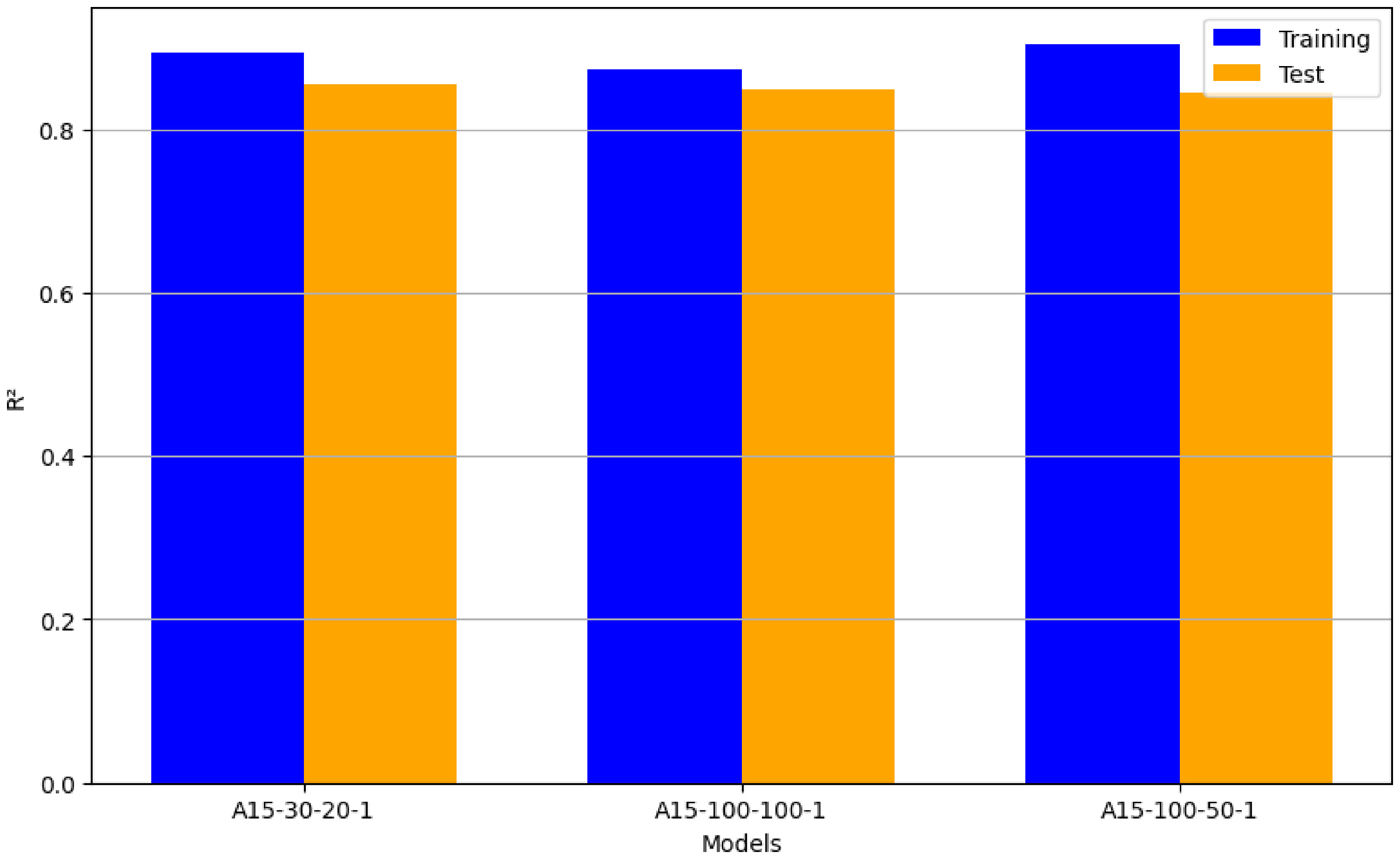
The analysis of the results reveals that the coefficients of determination (R²) on the training sets remained high, around 0.9 for all evaluated architectures, demonstrating the models' ability to capture the underlying patterns in the data, as shown in Figure 14. However, the discrepancy between R² values on the training and test sets indicates generalization capability. Among the analyzed architectures, A15-30-20-1 showed the slightest discrepancy between the sets, standing for more excellent stability. On the other hand, the A15-100-100-1 and A15-100-50-1 architectures exhibited more pronounced differences in R² values, indicating slight overfitting, although they still maintain satisfactory predictive performance.

Figure 14
Comparison of R² for training and testing the top three models with 2000 iterations.

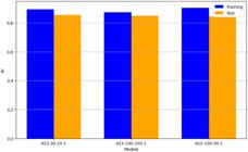
Table 4 presents the performance results of the three main neural network architectures evaluated based on metrics such as the coefficient of determination (R²), mean absolute error (MAE), root mean square error (RMSE), and mean absolute percentage error (MAPE). These data allow for a detailed comparison of each configuration's effectiveness.

Table 4
Performance metrics for different neural network architectures.

Metrics	Architectures
	A15-30-20-1	A15-100-100-1	A15-100-50-1
Activation Function	tanh	tanh	relu
Optimizer	lbfgs	lbfgs	lbfgs
R2 (Training)	89.79%	87.38%	90.50%
R2 (Test)	86.39%	84.93%	84.43%
MAE	13.5m	14.39m	14.82m
RMSE	19.6m	20.62m	20.96m
MAPE	25.00%	25.53%	26.12%

Among the tested architectures, A15-30-20-1 achieved the most balanced and robust performance. It obtained an R² of 89.79% on the training set and 86.39% on the test set, with the lowest RMSE (19.6 m) and MAPE (25.00%). These values indicate strong generalization capability, predictive efficiency, and a reliable fit to the analyzed data.

The A15-100-100-1 architecture performed slightly worse, with R² values of 87.38% (training) and 84.93% (test), alongside moderately higher RMSE (20.62 m) and MAPE (25.53%). Although still within an acceptable range, these results suggest a minor reduction in predictive power compared to the A15-30-20-1 model.

By contrast, A15-100-50-1 showed the highest R² on the training set (90.50%) but experienced a more pronounced drop on the test set (84.43%), suggesting overfitting, an excessive adjustment to the training data that limits generalization. This model also produced the highest RMSE (20.96 m) and MAPE (26.12%), reinforcing its lower predictive accuracy relative to the other two.

To contextualize the models’ accuracy within the scale of the dependent variable (wraparound device length), the RMSE was expressed as a percentage of the variable’s range (203 m, corresponding to 210 m – 7 m). The proportions were calculated as follows:

• A15-30-20-1: (19.6 / 203) × 100 ≈ 9.66%

• A15-100-100-1: (20.62 / 203) × 100 ≈ 10.16%

• A15-100-50-1: (20.96 / 203) × 100 ≈ 10.33%

These results show that the A15-30-20-1 architecture achieved the lowest RMSE proportion relative to the data scale (9.66%), reflecting superior predictive efficiency. While the values for A15-100-100-1 (10.16%) and A15-100-50-1 (10.33%) were slightly higher, they still fall within an acceptable range, typically between 10 and 15%, depending on the application context.

A more detailed assessment of the A15-30-20-1 model confirms its robustness:

1. Coefficient of Determination (R²): High values for both training (89.79%) and testing (86.39%) indicate excellent explanatory power with minimal loss of generalization.

2. Mean Absolute Error (MAE): An average deviation of 13.5 m between predictions and observed values demonstrates reliable predictive precision.

3. Root Mean Square Error (RMSE): With 19.6 m, the model maintains prediction errors well below 10% of the total variable range, confirming strong predictive efficiency.

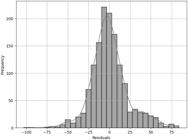
4. Residual Distribution: Residual analysis revealed an approximately symmetric distribution around zero, with density curves suggesting near-normal behavior and no significant systematic bias. While some extreme residuals were observed, likely due to data outliers or highly complex cases, the overall distribution confirms the model’s suitability for most of the analyzed data.

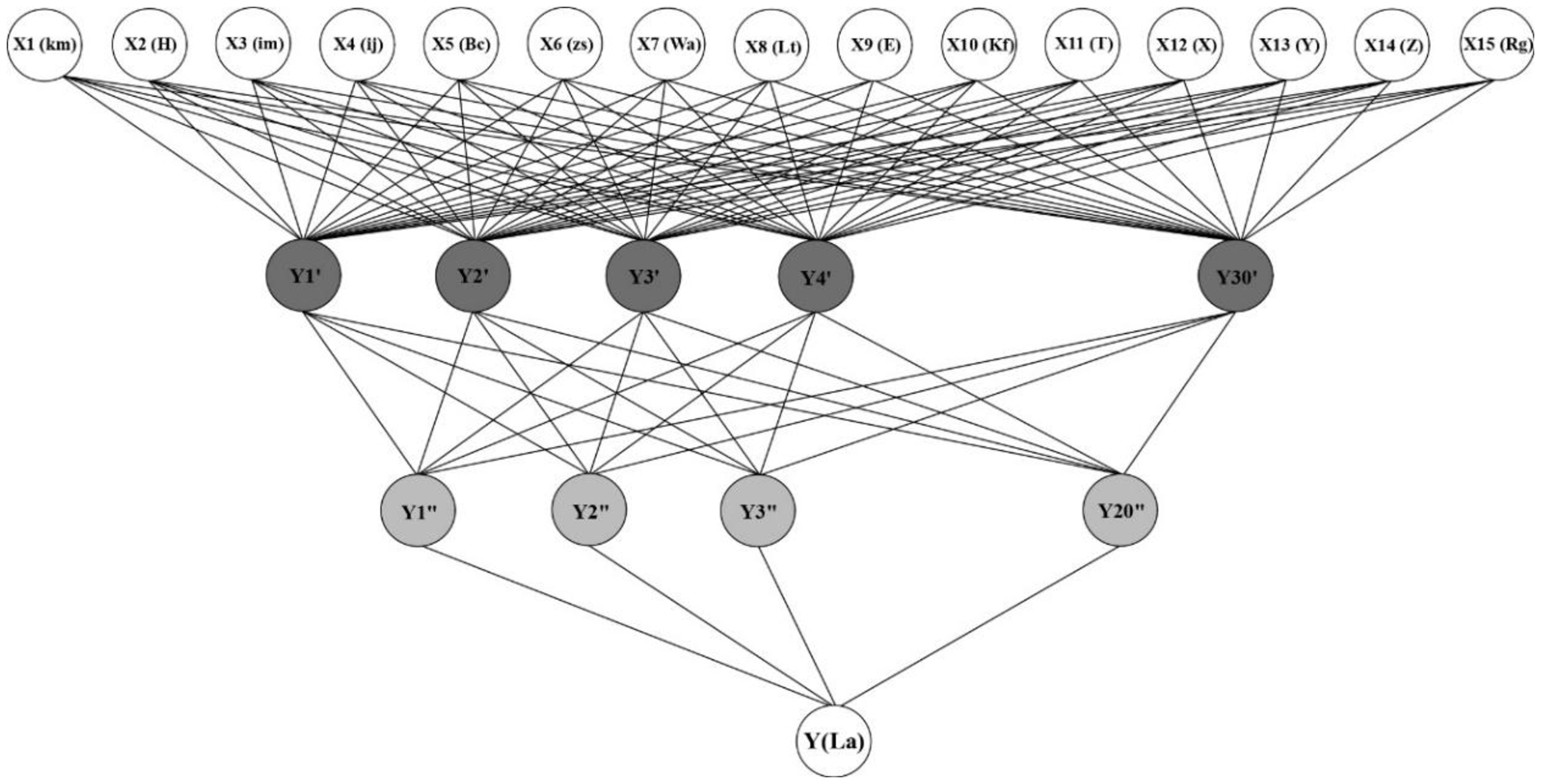
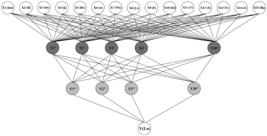
In summary, the A15-30-20-1 architecture (Figure 15) stands out as the most effective neural network configuration evaluated. Its combination of high R² values, low error metrics, and well-behaved residuals highlights its strong generalization capability and predictive reliability in estimating the wraparound device length in earth dams.

Figure 15
Best-Performing ANN Architecture: A15-30-20-1.

Cross-validation for the best-performing neural model

The metrics obtained from the cross-validation analysis confirm the performance of the A15-30-20-1 model, which was identified as the best architecture in the performance metrics evaluation. During the cross-validation process, this model achieved an average coefficient of determination (R²) of 0.8377, demonstrating that, on average, it could explain 83.77% of the data variability across the different subsets analyzed. This result highlights the model's efficiency in capturing the underlying patterns of the data, ensuring a high level of generalization even when faced with different dataset partitions.

Additionally, the standard deviation of the R² values was 0.0153, indicating low dispersion in the performance obtained for each cross-validation fold. This low variability suggests that the A15-30-20-1 model exhibits consistency and stability, showing minimal sensitivity to variations between the training and testing subsets.

Feature importance in the MLP model

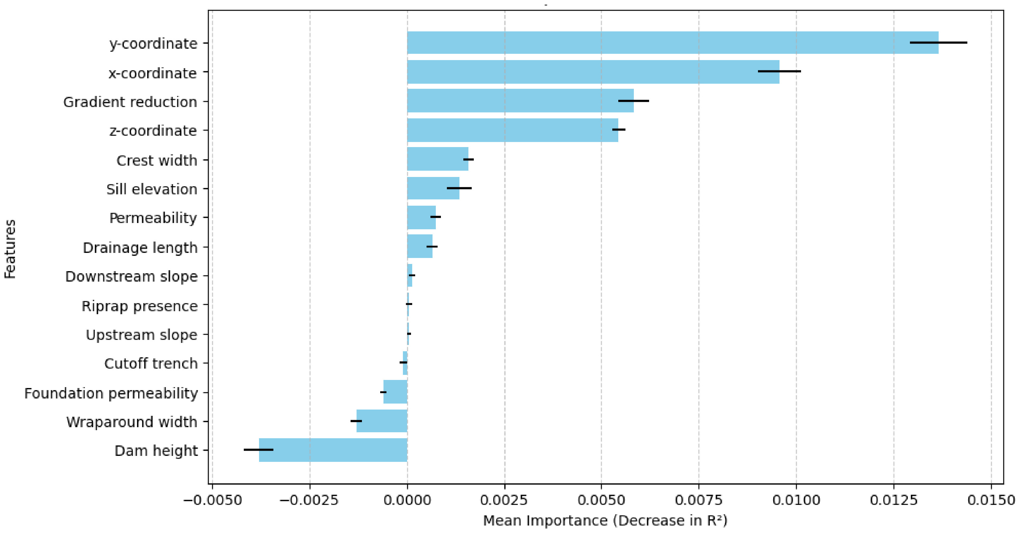
The model identified the spatial coordinates x, y, and z, representing the locations where the hydraulic gradient was measured, as the most influential variables for predicting the wraparound length. These variables had the strongest impact on the model’s predictions, indicating that the spatial position within the dam is a key determinant for determining the required wraparound length. The reduction of the hydraulic gradient due to the implementation of the wraparound device also showed a moderate effect, though less pronounced than the spatial coordinates.

Variables such as crest width, sill elevation, soil permeability, and drainage length exhibited moderate influence, suggesting that geometric and hydraulic properties contribute to variations in wraparound length but are secondary to spatial factors. In contrast, downstream slope, riprap presence, upstream slope, cutoff trench, foundation permeability, wraparound width, and dam height had low or negligible impact on predictions, implying that these factors play a minor role in determining wraparound length or may introduce noise.

Overall, these results, presented in Figure 16, indicate that the model primarily relies on spatial information to predict wraparound length, while geometric and structural parameters have limited influence. This highlights the critical role of measurement location and the moderate effectiveness of the wraparound device in influencing hydraulic gradient management within the dam.

Figure 16
Influence of each input on the network response.

Residual analysis for the best-performing neural model

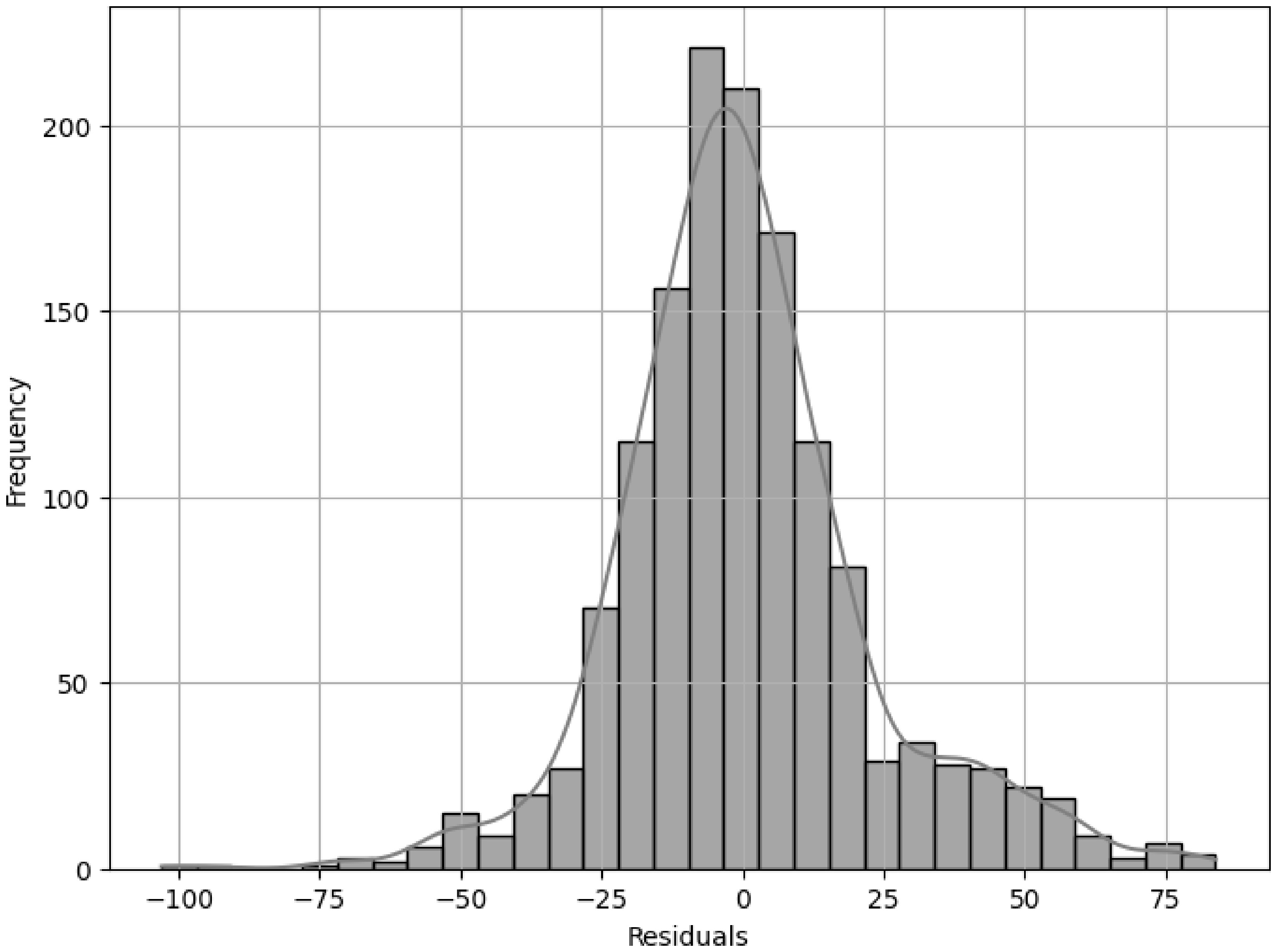
The histogram analysis (Figure 17) for the A15-30-20-1 model reveals an approximately symmetric distribution of residuals centered around zero, indicating the absence of systematic bias in the predictions. This behavior suggests that the errors are balanced, with no predominant tendency for overestimation or underestimation, reflecting the quality of the model's fit. The density curve overlaid on the histogram further reinforces the adherence of the residuals to a normal distribution. However, extreme residuals indicate potential outliers in the data or limitations of the model in capturing complex patterns in specific cases.

Figure 17
Residual histogram for the A15-30-20-1 architecture.

Practical limitations and efficiency gains of the hybrid MEF–machine learning approach in dam engineering

The integrated approach combining three-dimensional Finite Element Method (FEM) simulations with machine learning (ML) techniques offers significant computational efficiency gains compared to relying solely on conventional FEM analyses for the design of control devices in dams. FEM provides detailed simulations of geotechnical and hydraulic behavior, allowing for a comprehensive assessment of flow under diverse conditions. However, three-dimensional FEM simulations are computationally intensive and time-consuming. Performing a full FEM simulation for each new design scenario would be prohibitively slow and expensive, which motivated the adoption of numerical simplifications in the model.

By generating a robust dataset with FEM simulations covering a wide range of geotechnical, hydraulic, and geometric conditions, and then training ML models on this dataset, the methodology allows almost instantaneous prediction of the optimal wraparound length for new dam configurations without requiring repeated costly FEM runs. Machine learning techniques, particularly Artificial Neural Networks (ANNs), are capable of capturing nonlinear and highly complex relationships between input variables (dam and soil parameters) and the output variable (wraparound length). Once trained, these models generalize effectively, providing accurate predictions for unseen scenarios without requiring extensive recalculations. Each ML approach offers specific advantages: ANNs are highly flexible and can model intricate data patterns, although they demand greater computational resources during training. Overall, the hybrid FEM–ML methodology constitutes an efficient and economically viable approach, replacing the need for repeated FEM simulations with rapid predictions generated by a trained ML model.

Despite these benefits, several practical limitations must be considered before applying the models in real-world dam engineering projects. The models were trained exclusively on synthetic FEM-generated data rather than experimental or field measurements. Without empirical validation, the reliability of predictions under actual operational conditions remains uncertain. Furthermore, the FEM simulations relied on assumptions of embankment homogeneity and fixed anisotropy ratios, which may not fully capture the complexity and variability of real-world dams, including heterogeneous soils, stratified layers, or complex anisotropic behavior. Additionally, while the models demonstrate good accuracy on synthetic datasets, their “black-box” nature limits interpretability. Geotechnical engineers require a clear understanding of causal relationships to make informed decisions in the field. The absence of real-time monitoring data and the lack of consideration for dynamic factors, such as flood cycles or extreme weather events, further restrict the extrapolation of predictions to operational scenarios.

A promising avenue to overcome these limitations lies in the integration of the proposed hybrid system with dam safety monitoring frameworks. Such integration would enable real-time updates of predictive models and more robust risk assessments, directly supporting dam safety management.

First, real-time updates and continuous monitoring could be achieved by incorporating data from in-field instrumentation, such as piezometers, seepage flow meters, and automated water level sensors. These empirical datasets are essential for validating and recalibrating the predictive models, thereby enhancing both accuracy and applicability in operational contexts. In practice, this integration would allow continuous verification of the model’s predictions regarding the optimal wraparound length, dynamically adjusting results in accordance with the actual hydraulic performance of the dam.

Second, dynamic and real-world complexities could be better represented. At present, the FEM–ML approach does not explicitly account for transient and evolving conditions, such as reservoir filling and drawdown cycles, extreme hydrological events linked to climate variability, or progressive processes such as internal erosion and crack propagation. By coupling predictive models with monitoring data streams, it becomes possible to incorporate transient flow simulations, heterogeneous soil structures with anisotropic permeability, and deterioration effects over time, thereby expanding the operational relevance of the methodology.

Third, enhanced risk assessment would be facilitated through continuous model refinement. The primary purpose of the hybrid FEM–ML model is to optimize percolation control devices and mitigate critical hydraulic gradients that may trigger internal erosion and compromise dam safety. With access to field monitoring data in real time, predictions could be iteratively validated and refined, providing engineers and regulatory agencies with a more precise and continuously updated risk profile. This integration would not only support more informed decision-making but also enable proactive interventions, such as operational adjustments or preventative engineering measures, before critical safety thresholds are reached.

In summary, while the hybrid FEM–ML methodology already provides substantial efficiency gains for dam design by reducing computational costs and enabling rapid scenario evaluation, its full potential will only be realized through systematic integration with real-time dam monitoring systems. Such integration will bridge the current gap between synthetic simulation-based predictions and real-world operational complexity, ensuring more reliable, interpretable, and actionable insights for dam safety management. Future studies must prioritize this empirical validation and integration to consolidate the hybrid approach as a practical tool for both design optimization and real-time risk assessment in dam engineering.

CONCLUSIONS

This paper presented an innovative approach for sizing internal percolation control devices in earth dams using Multilayer Perceptron Artificial Neural Networks (ANNs). The proposed methodology integrated three-dimensional numerical simulations of water flow, conducted through the Finite Element Method (FEM), with machine learning techniques to optimize the sizing of percolation control devices, known as wraparound. The study demonstrated that applying ANNs is a promising tool for geotechnical engineering, particularly in scenarios where the complexity of interactions between geometric, hydraulic, and geotechnical parameters demands sophisticated approaches.

The analysis of the results revealed that the ANN model configured with two hidden layers containing 30 and 20 neurons, respectively (architecture A15-30-20-1), exhibited the best overall performance. This model achieved a coefficient of determination (R²) of 89.79% on the training set and 86.39% on the test set, demonstrating a high generalization capability and accuracy in predicting the optimal wraparound length. Additionally, the model recorded the lowest values of Root Mean Square Error (RMSE) and Mean Absolute Percentage Error (MAPE), indicating a minor discrepancy between actual and predicted values. The proportion of RMSE relative to the range of the dependent variable was approximately 9.66%, further reinforcing the model's efficiency within the analyzed scale.

Cross-validation confirmed the robustness of the A15-30-20-1 model, with an average coefficient of determination (R²) of 0.8377 and a standard deviation of 0.0153, indicating consistency and stability across different data partitions. The residual analysis showed an approximately symmetric distribution with no systematic bias, suggesting that the model can adequately capture the underlying patterns in the data. However, some extreme residuals indicate potential limitations in specific cases.

Compared to other tested architectures, such as A15-100-100-1 and A15-100-50-1, the A15-30-20-1 model stood out for its ability to balance computational complexity with predictive effectiveness. While architectures with more neurons showed signs of overfitting, the A15-30-20-1 model maintained consistent performance across training and validation, demonstrating a better ability to generalize to new data.

In summary, the approach proposed in this paper offers a well-founded technical solution for sizing percolation control devices in earth dams, addressing a significant gap in the scientific literature and providing practical support for engineers involved in designing and constructing these structures. The use of ANNs, combined with three-dimensional numerical simulations, proved effective in capturing complex and nonlinear relationships between variables, optimizing wraparound length, and mitigating critical hydraulic gradients. Future work could explore the application of this methodology to other types of dams or scenarios with more significant geotechnical variability and investigate the impact of different activation functions and optimization algorithms on model performance.

DATA AVAILABILITY STATEMENT

Research data is only available upon request.

ACKNOWLEDGEMENTS

I would like to thank the Graduate Program in Geotechnics of the Department of Hydraulic and Environmental Engineering at the Federal University of Ceará (DEHA-UFC) for the valuable opportunities it provided and the Coordination for the Improvement of Higher Education Personnel (CAPES) for the essential financial support that made this work possible, grant number 88887.826088/2023-00.

Appendix A Code for training and evaluating different artificial neural network configurations

A.1 Importing Modules and Loading Data

# Import necessary modules

import numpy as np

import pandas as pd

import matplotlib.pyplot as plt

import seaborn as sns

from sklearn.preprocessing import RobustScaler, StandardScaler, MinMaxScaler

from sklearn.decomposition import PCA

from sklearn.neural_network import MLPRegressor

from sklearn.metrics import mean_absolute_error, mean_squared_error, explained_variance_score, r2_score

from sklearn.model_selection import KFold, cross_val_score, GridSearchCV, train_test_split, learning_curve

# Load dataset

df2 = pd.read_csv('/content/drive/MyDrive/doutorado/dados_10.csv', sep=',', encoding='iso-8859-1')

df = df2.dropna()

# Separate independent and dependent variables

X = df.iloc[:, 0:16].values

y = df.iloc[:, 16].values

A.2 Data Preprocessing

# Split data into training and testing sets

x_train, x_test, y_train, y_test = train_test_split(X, y, test_size=0.2, random_state=42)

# Normalize input features

x_scaler = MinMaxScaler()

x_train_scaled = x_scaler.fit_transform(x_train)

x_test_scaled = x_scaler.transform(x_test)

# Normalize output variable

y_scaler = MinMaxScaler()

y_train_scaled = y_scaler.fit_transform(y_train.reshape(-1, 1))

y_test_scaled = y_scaler.transform(y_test.reshape(-1, 1))

A.3 Model Training and Evaluation

# Define model configurations

activation_functions = ['relu', 'logistic', 'tanh']

solvers = ['adam', 'lbfgs']

hidden_layer_configurations = [(7, 7, 7), (10, 10), (30, 20), (50, 50), (100, 50), (100, 100), (100,)]

# Loop to train models with different configurations

results = []

for activation in activation_functions:

for solver in solvers:

for hidden_layer_sizes in hidden_layer_configurations:

print(f"Training model with activation={activation}, solver={solver}, layers={hidden_layer_sizes}")

try: model = MLPRegressor( hidden_layer_sizes=hidden_layer_sizes, activation=activation, solver=solver, max_iter=2000, random_state=42 ) model.fit(x_train_scaled, y_train_scaled.ravel()) # Model evaluation r2_train = model.score(x_train_scaled, y_train_scaled) r2_test = model.score(x_test_scaled, y_test_scaled) y_pred_scaled = model.predict(x_test_scaled) y_pred_inverse = y_scaler.inverse_transform(y_pred_scaled.reshape(-1, 1)) # Calculate metrics mae = mean_absolute_error(y_test, y_pred_inverse) rmse = np.sqrt(mean_squared_error(y_test, y_pred_inverse)) mape = np.mean(np.abs((y_test - y_pred_inverse.flatten()) / y_test)) * 100 explained_var = explained_variance_score(y_test, y_pred_inverse) # Store results results.append({ 'activation': activation, 'solver': solver, 'hidden_layer_sizes': hidden_layer_sizes, 'r2_train': r2_train, 'r2_test': r2_test, 'mae': mae, 'rmse': rmse, 'mape': mape, 'explained_variance': explained_var }) except Exception as e: print(f"Error training model: {e}")

A.4 Visualization and Analysis of Results

# Train the best model

best_model = MLPRegressor( hidden_layer_sizes=(30, 20), activation='tanh', solver='lbfgs', max_iter=2000, random_state=42)

best_model.fit(x_train_scaled, y_train_scaled.ravel())

# Predictions and residuals

y_pred_scaled = best_model.predict(x_test_scaled)

y_pred_inverse = y_scaler.inverse_transform(y_pred_scaled.reshape(-1, 1))

residuals = y_test - y_pred_inverse.flatten()

# Scatter plot: Actual vs Predicted

plt.figure(figsize=(8, 6))

plt.scatter(y_test, y_pred_inverse, alpha=0.7, color="blue")

plt.plot([y_test.min(), y_test.max()], [y_test.min(), y_test.max()], color="red", linestyle="--", linewidth=2)

plt.title("Actual vs Predicted Values (Best Model)")

plt.xlabel("Actual Values")

plt.ylabel("Predicted Values")

plt.grid()

plt.show()

# Histogram of residuals

plt.figure(figsize=(8, 6))

sns.histplot(residuals, kde=True, bins=30, color='gray', alpha=0.7)

plt.title("Residuals Histogram: Best Model")

plt.xlabel("Residuals")

plt.ylabel("Frequency")

plt.grid()

plt.show()

# Comparison of R² for the top three models

models = ["Best Model", "Second Best Model", "Third Best Model"]

r2_train_vals = [ best_model.score(x_train_scaled, y_train_scaled), second_model.score(x_train_scaled, y_train_scaled), third_model.score(x_train_scaled, y_train_scaled)]

r2_test_vals = [ best_model.score(x_test_scaled, y_test_scaled), second_model.score(x_test_scaled, y_test_scaled), third_model.score(x_test_scaled, y_test_scaled)]

# Bar chart x = np.arange(len(models)) width = 0.35

plt.figure(figsize=(10, 6))

plt.bar(x - width/2, r2_train_vals, width, label="Training", color="blue")

plt.bar(x + width/2, r2_test_vals, width, label="Testing", color="orange")

plt.title("R² Comparison (Training vs Testing) of the Top Three Models")

plt.xlabel("Models")

plt.ylabel("R²")

plt.xticks(x, models)

plt.legend()

plt.grid(axis="y")

plt.show()

REFERENCES

• Ali, M. M. (2021). Modified limited-memory Broyden-Fletcher-Goldfarb-Shanno algorithm for unconstrained optimization problem. Indonesian Journal of Electrical Engineering and Computer Science, 24, 1027.
• Beiranvand, B., & Rajaee, T. (2022). Application of artificial intelligence-based single and hybrid models in predicting seepage and pore water pressure of dams: A state-of-the-art review. Advances in Engineering Software, 173, 103268.
• Brasil. (2010). Lei nº 12.334, de 20 de setembro de 2010. Lei de Segurança de Barragens.Diário Oficial [da] República Federativa do Brasil, Brasília, seção 1. Retrieved in 2025, February 20, fromhttp://www.planalto.gov.br/ccivil_03/_Ato2007-2010/2010/Lei/L12334.htm
  » http://www.planalto.gov.br/ccivil_03/_Ato2007-2010/2010/Lei/L12334.htm
• Dawson, C. W., & Wilby, R. L. (2001). Hydrological modelling using artificial neural networks. Progress in Physical Geography, 25(1), 80-108.
• Demuth, H. B., Beale, M. H., De Jess, O., & Hagan, M. T. (2014).Neural network design (2nd ed.). Stillwater, OK: Martin Hagan.
• Géron, A. (2022).Hands-on machine learning with Scikit-Learn, Keras, and TensorFlow Sebastopol, CA: O’Reilly Media, Inc.
• Glorot, X., Bordes, A., & Bengio, Y. (2011). Deep sparse rectifier neural networks. In G. Gordon, D. Dunson, & M. Dudík (Eds.), Proceedings of the Fourteenth International Conference on Artificial Intelligence and Statistics (pp. 315-323). Cambridge, MA: ML Research Press.
• Goodfellow, I., Bengio, Y., & Courville, A. (2016).Deep learning Cambridge, MA: MIT Press.
• Hamedi, S., Dehdashti Jahromi, H., & Lotfiani, A. (2023). Artificial intelligence-aided nanoplasmonic biosensor modeling. Engineering Applications of Artificial Intelligence, 118, 105646.
• Hamedi, S., & Dehdashti Jahromi, H. (2021). Performance analysis of all-optical logical gate using artificial neural network. Expert Systems with Applications, 178, 115029.
• Hastie, T. (2009). The elements of statistical learning: data mining, inference, and prediction. Berlin: Springer.
• Haykin, S. (2001).Redes neurais: Princípios e prática Porto Alegre: Bookman Editora.
• Iacomcafé. (2025). A importância da validação cruzada em Machine Learning Retrieved in 2025, February 20, fromhttps://iacomcafe.com.br/importancia-validacao-cruzada-machine-learning/
  » https://iacomcafe.com.br/importancia-validacao-cruzada-machine-learning/
• IPNET. (2023). A importância da normalização e padronização dos dados em machine learning Retrieved in 2025, February 18, from https://medium.com/ipnet-growth-partner/padronizacao-normalizacao-dados-machine-learning-f8f29246c12
  » https://medium.com/ipnet-growth-partner/padronizacao-normalizacao-dados-machine-learning-f8f29246c12
• Jain, A. K., Mao, J., & Mohiuddin, K. M. (1996). Artificial neural networks: A tutorial. Computer, 29(3), 31-44.
• Jahromi, H. D., & Hamedi, S. (2021). Artificial intelligence approach for calculating electronic and optical properties of nanocomposites. Materials Research Bulletin, 141, 111371.
• Jin, W., Liu, S., & Wang, K. (2022). Internal erosion experiments on sandy gravel alluvium in an embankment dam foundation emphasizing horizontal seepage and high surcharge pressure. Water, 14(20), 3285.
• Ke, L., & Takahashi, A. (2014). Experimental investigations on suffusion characteristics and its mechanical consequences on saturated cohesionless soil. Soil and Foundation, 54, 713-730.
• Kingma, D. P., & Ba, J. (2015). Adam: A method for stochastic optimization. In International Conference on Learning Representations (ICLR) San Diego: ICLR.
• Kohavi, R. (1995). A study of cross-validation and bootstrap for accuracy estimation and model selection. In Proceedings of the 14th International Joint Conference on Artificial Intelligence (IJCAI) (pp. 1137-1143). Montreal: IJCAI.
• Lederer, J. (2021). Activation functions in artificial neural networks: A systematic overview.arXiv preprint
• Maier, H. R., & Dandy, G. C. (2000). Neural networks for the prediction and forecasting of water resources variables: A review of modelling issues and applications. Environmental Modelling & Software, 15(1), 101-124.
• McCulloch, W. S., & Pitts, W. A. (1943). A logical calculus of the ideas immanent in nervous activity. The Bulletin of Mathematical Biophysics, 5, 115-133.
• Miranda, S. A. (2009).Análise paramétrica do regime de fluxo numa barragem de terra assente em solos permeáveis: Estudo de caso: PCH Canoa Quebrada (Dissertação de mestrado). Universidade Federal de Ouro Preto, Ouro Preto.
• Nocedal, J. (1980). Updating quasi-Newton matrices with limited storage. Mathematics of Computation, 35(151), 773-782.
• Pedregosa, F., Varoquaux, G., Gramfort, A., Michel, V., Thirion, B., Grisel, O., & Blondel, M. (2011). Scikit-learn: Machine learning in Python. Journal of Machine Learning Research, 12, 2825-2830.
• Poso, F. D., & De Jesus, K. L. M. (2022). Neural network-particle swarm optimization model for predicting slope stability of homogeneous earth dams. In 2022 IEEE 14th International Conference on Humanoid, Nanotechnology, Information Technology, Communication and Control, Environment, and Management (HNICEM) New York: IEEE.
• RETEC. (2009).Soil hydraulic and retention models, version 6.02 RETEC Software.
• Rumelhart, D. E., Hinton, G. E., & Williams, R. J. (1986). Learning representations by back-propagating errors. Nature, 323(6088), 533-536.
• Salgado, S. R. T., Carvalho, E., Viseu, M. T., & Oliveira, O. F. (2025). Evaluating dam safety in Brazil: a comparative analysis of international classification systems. Revista Brasileira de Recursos Hídricos, 30, e46.
• Salazar, F., Toledo, M. A., Oñate, E., & Morán, R. (2015). An empirical comparison of machine learning techniques for dam behaviour modelling. Structural Safety, 56, 9-17.
• Saré, A. R. (2003).Análise das condições de fluxo na barragem de Curuá-Una, Pará (Dissertação de mestrado). Pontifícia Universidade Católica, Rio de Janeiro.
• Seequent. (2024). GeoStudio (Version 24.2.1) [Software]. Bentley Systems. Retrieved in 2025, February 18, from https://www.seequent.com/products-solutions/geostudio/
  » https://www.seequent.com/products-solutions/geostudio/
• Silva, A. C., Silva, F. G. B., Valério, V. E. M., Silva, A. T. Y. L., Marques, S. M., & Reis, J. A. T. (2024). Application of data prediction models in a real water supply network: comparison between arima and artificial neural networks. Revista Brasileira de Recursos Hídricos, 29, e12.
• Silva, D. L., Jesus, K. L. M., Adina, E. M., Mangrobang, D. V., Escalante, M. D., & Susi, N. A. M. (2021). Prediction of tensile strength and erosional effectiveness of natural geotextiles using artificial neural network. In 2021 13th International Conference on Computer and Automation Engineering (ICCAE) (pp. 121-127). New York: IEEE.
• Sousa, A. D. (2013). Analise do comportamento hidraulico em interfaces solo/estrutura em barragens de terra. Revista de Engenharia Geotecnica, 35(2), 45-59.
• Souza, R. G. M., Brentan, B. M., & Lima, G. M. (2021). Optimal architecture for artificial neural networks as pressure estimator. Revista Brasileira de Recursos Hídricos, 26, e37.
• Tayfur, G., Swiatek, D., Wita, A., & Singh, V. P. (2005). Case study: finite element and artificial neural network models for flow through Jeziorsko earthfill dam in Poland. Journal of Hydraulic Engineering, 131(6), 431-440.
• Topok, Z. F., & Cigizoglu, H. K. (2008). Predicting longitudinal dispersion coefficient in natural streams by artificial intelligence methods. Hydrological Processes, 22(20), 4106-4129.
• Ünes, F. (2021). Dam reservoir level modeling by neural network approach: A case study. Neural Network World, 31(2), 123-132.
• Van Genuchten, M. T. (1980). A closed-form equation for predicting the hydraulic conductivity of unsaturated soils. Soil Science Society of America Journal, 44(5), 892-898.
• Xu, Z. X., & Li, J. Y. (2002). Short-term inflow forecasting using an artificial neural network model. Hydrological Processes, 16(12), 2423-2439.
• Xue, X., Yang, X., & Chen, X. (2014). Estimating piping potential in earth dams and levees using generalized neural networks. Acta Geotechnica Slovenica, 11(2), 59-69.

Edited by

• Editor-in-Chief:
  Adilson Pinheiro

• Associated Editor:
  Edson Cezar Wendland

Publication Dates

• Publication in this collection
  20 Apr 2026
• Date of issue
  2026

History

• Received
  20 Feb 2025
• Reviewed
  27 Jan 2026
• Accepted
  28 Jan 2026