Figure 1
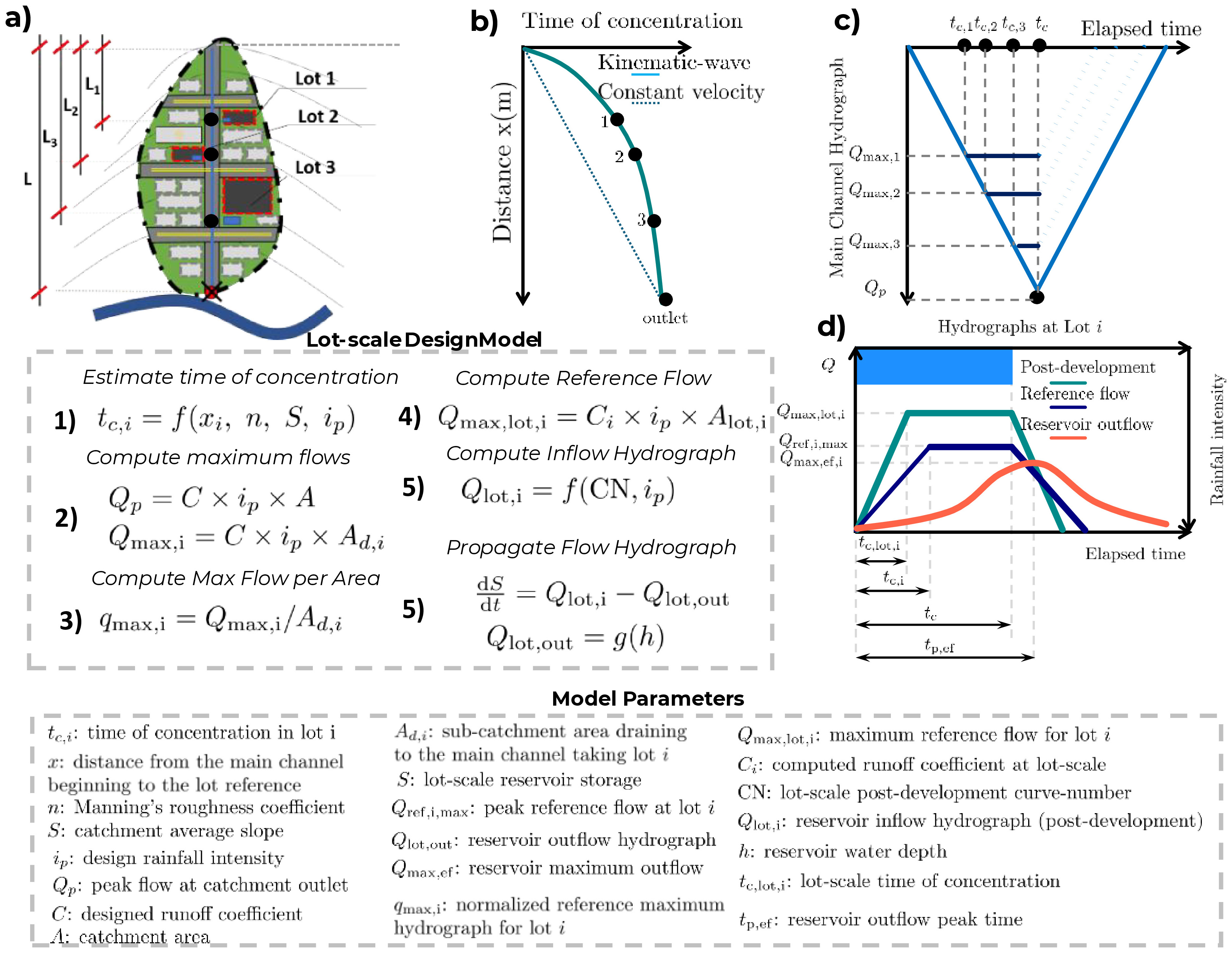
Problem schematics, where (a) shows a plan representation of a small, urbanized catchment with a main urban drainage channel. Distances L are taken from the main channel reference. Grey dashed boxes represent residential areas, whereas black, red dashed boxes represent lots that will be designed in the examples presented in this manuscript. The blue box represents a small rectangular detention pond, and the red crossed circle is the catchment outlet. In (b), a schematic of the non-linear kinematic-wave time of concentration is shown, indicating this variable for lots 1, 2, 3, and for the outlet. For reference, a constant-velocity scheme is contrasted with deviations from a simpler time-of-concentration method toward a physically based approach. Part (c) shows the hydrograph at section x1, x2, x3 (representing the lots' position), and at the outlet. If normalized by their upstream sub-catchment area, these hydrographs can represent the maximum flow discharge per area that a lot can convey to the receptor drainage system. The dark blue lines indicate a constant-flow hydrograph due to rainfall duration exceeding the reference time of concentration, and the dotted cyan lines are the recession hydrographs at these sections. The brief summary of the pseudocode for the simulation is shown in steps (1) to (5) with model parameters below, later fully described in the paper, and part (d) shows a schematic representation of the flow propagation in a lot-scale reservoir designed with the methods presented in this paper.
Figure 2
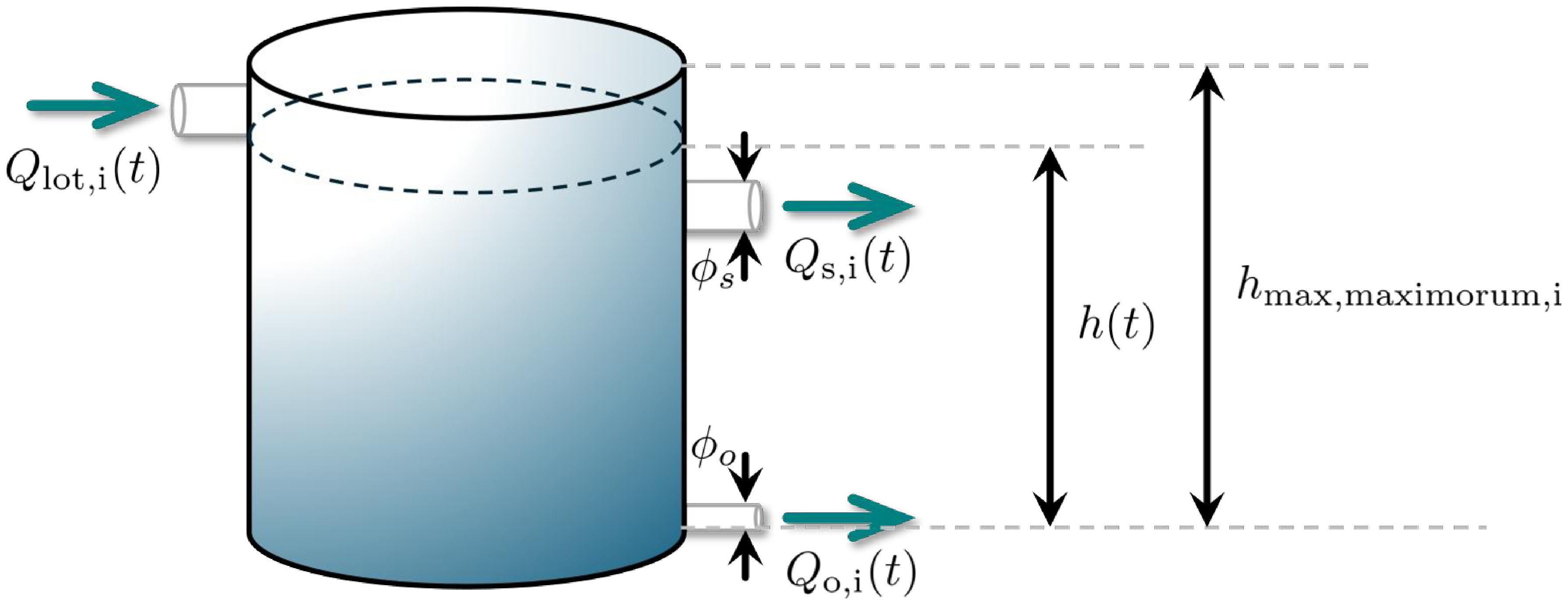
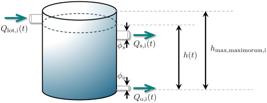
Lot-scale reservoir and its hydraulic devices for a double outlet where ϕs, ϕh, are the diameter of the orifice and spillway, respectively, and h(t) is the water depth. The maximorum height (hmax,maximorum) defines the maximum water depth h. The orifice is assumed to be without any internal water storage below, and the spillway centerline is defined at the elevation cs from the reservoir bottom.
Figure 3
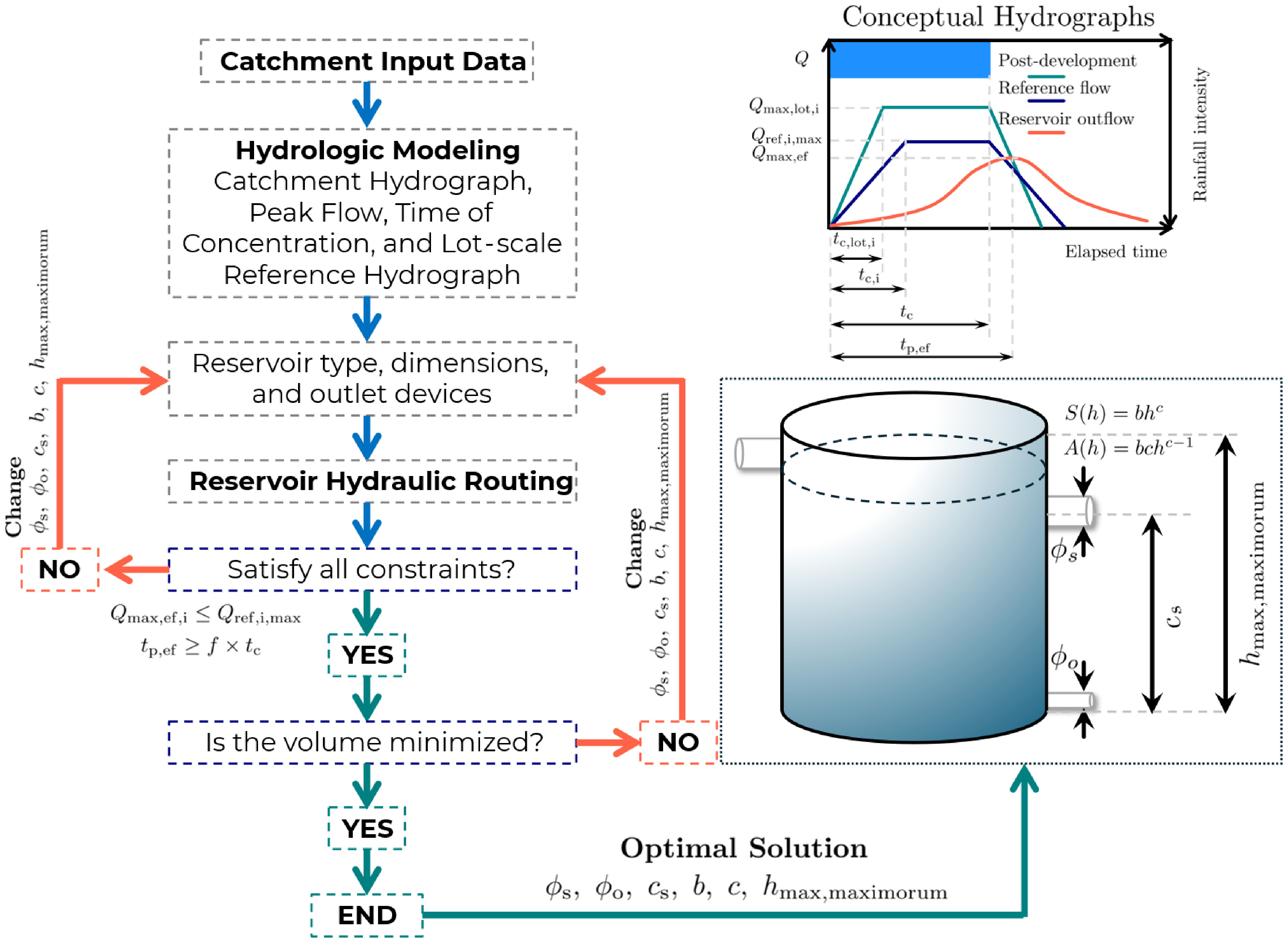
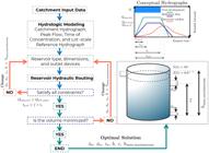
Design of lot-scale reservoir flowchart.
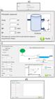
Figure 4
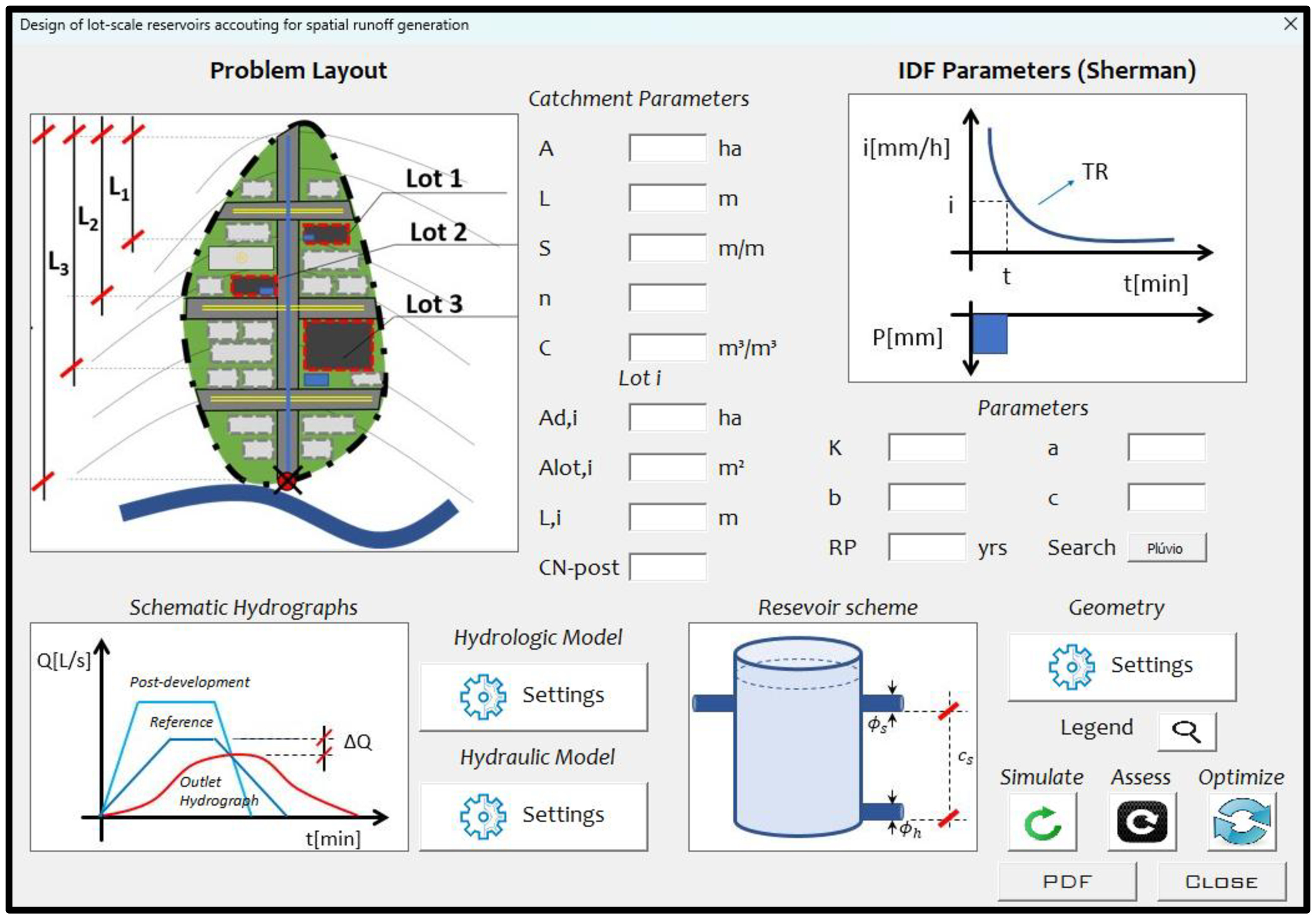
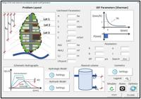
Main Guided User Interface (GUI) of the developed tool. The gray rectangular boxes in the schematic catchment represent residential or commercial lots, whereas red-dashed black boxes are fully impervious areas that require lot-scale reservoirs to mitigate excess of runoff. The main input files are the Catchment Parameters - which define the catchment and lot properties, followed by the toolboxes Hydrologic Model and Hydraulic Model Geometry input data.
Figure 5
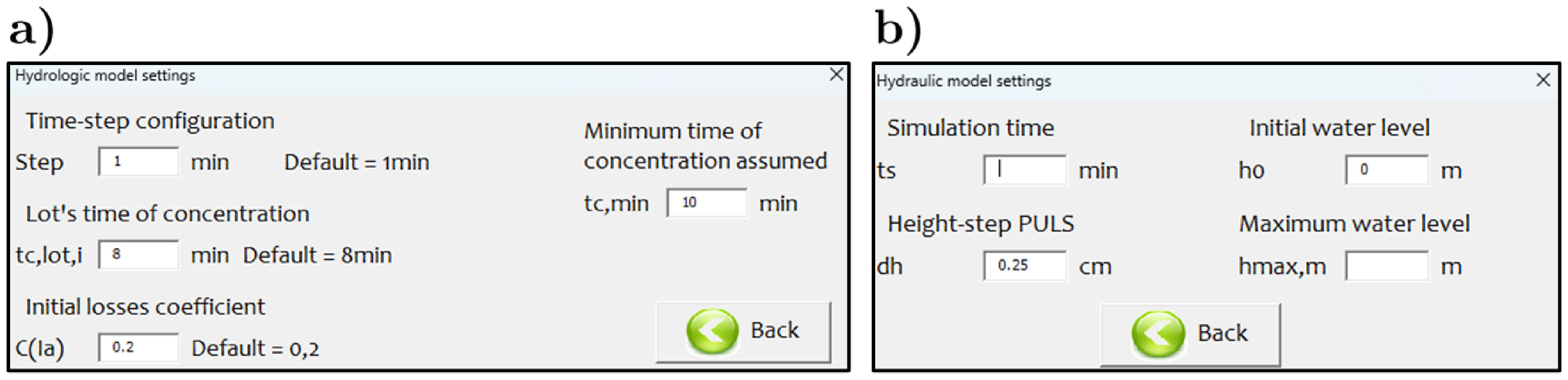
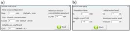
Hydrologic (a) and Hydraulic settings (b) where one can set time-step, lot-scale time of concentration, initial losses coefficient, simulation time, solver time, space discretization, initial conditions, and maximum depth.
Figure 6
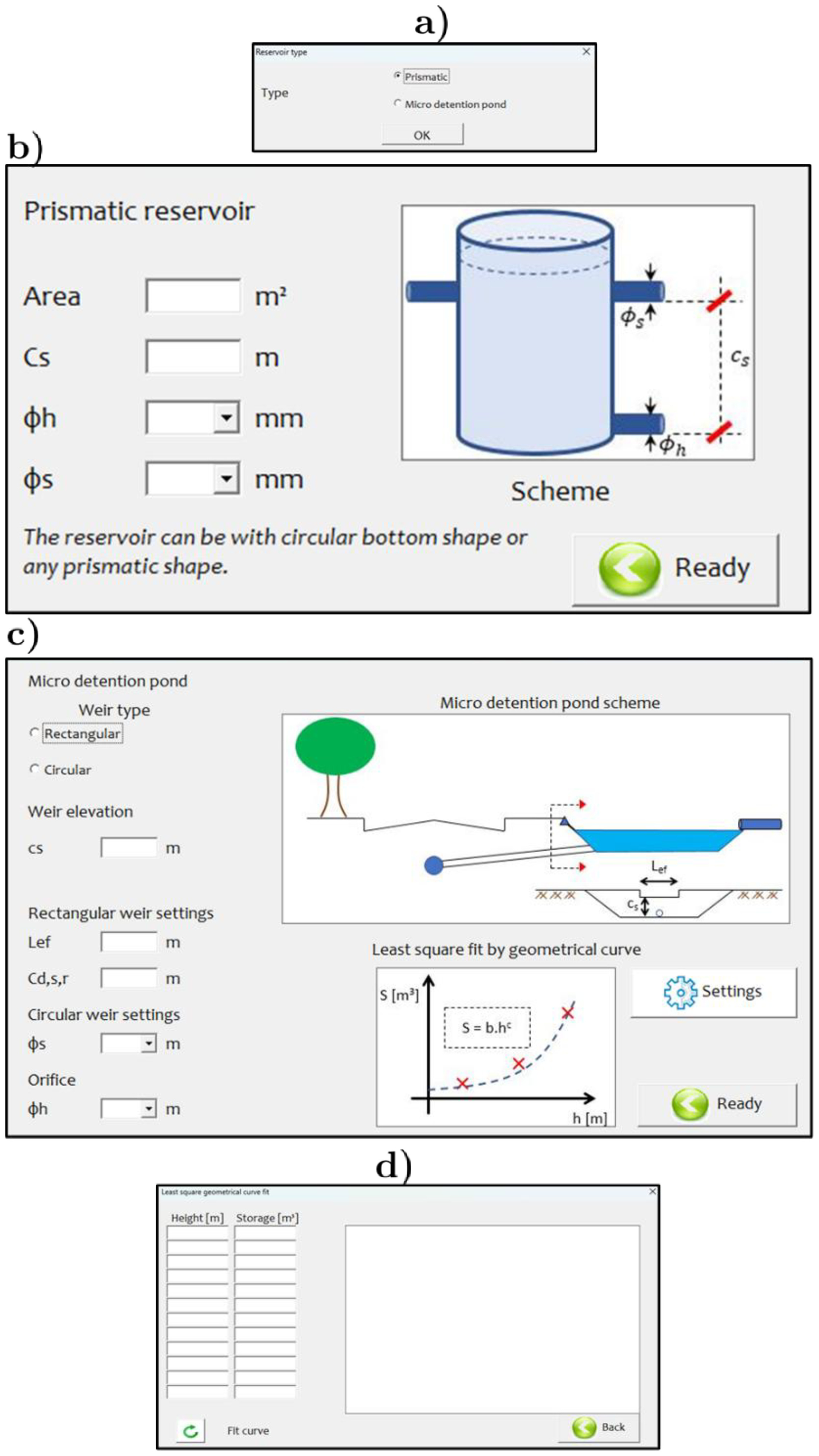
Lot-scale reservoir geometry settings, where (a) allows users to change reservoir shape, (b) shows the prismatic reservoir interface, (c) shows the micro detention pond shape, and (d) shows the tabular stage-storage input data for the micro detention design toolkit.
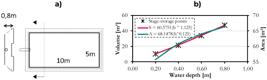
Figure 7
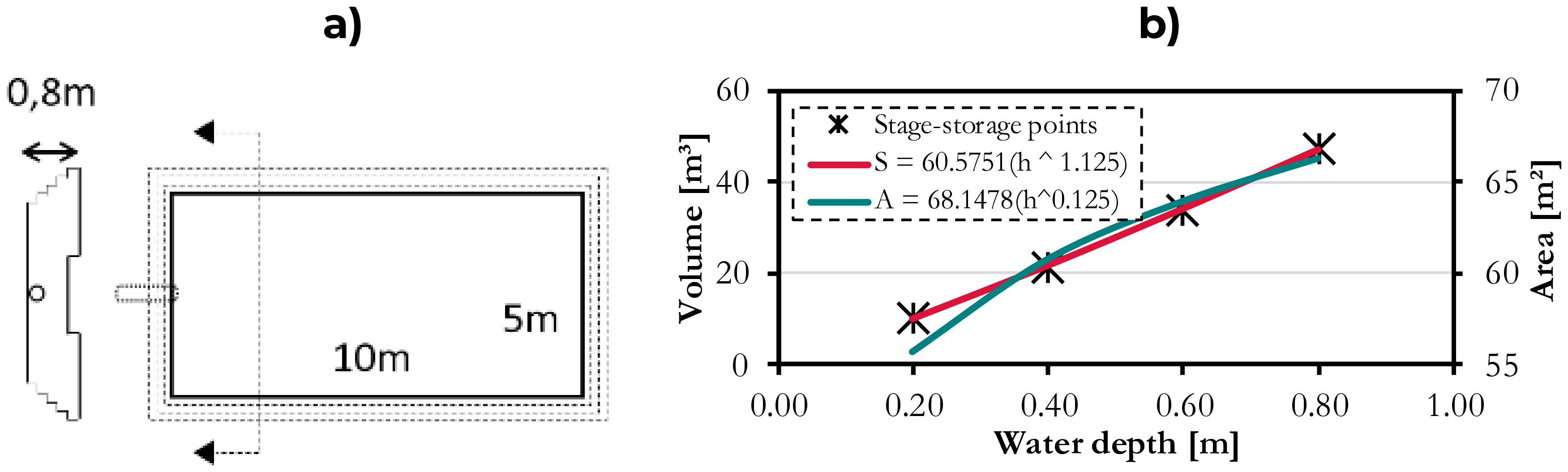
(a) Reservoir schematics plan view and (b) least-square stage-storage-area fit.
Figure 2
Lot-scale reservoir and its hydraulic devices for a double outlet where ϕs, ϕh, are the diameter of the orifice and spillway, respectively, and h(t) is the water depth. The maximorum height (hmax,maximorum) defines the maximum water depth h. The orifice is assumed to be without any internal water storage below, and the spillway centerline is defined at the elevation cs from the reservoir bottom.
Figure 3
Design of lot-scale reservoir flowchart.
Figure 4
Main Guided User Interface (GUI) of the developed tool. The gray rectangular boxes in the schematic catchment represent residential or commercial lots, whereas red-dashed black boxes are fully impervious areas that require lot-scale reservoirs to mitigate excess of runoff. The main input files are the Catchment Parameters - which define the catchment and lot properties, followed by the toolboxes Hydrologic Model and Hydraulic Model Geometry input data.
Figure 5
Hydrologic (a) and Hydraulic settings (b) where one can set time-step, lot-scale time of concentration, initial losses coefficient, simulation time, solver time, space discretization, initial conditions, and maximum depth.
Figure 6
Lot-scale reservoir geometry settings, where (a) allows users to change reservoir shape, (b) shows the prismatic reservoir interface, (c) shows the micro detention pond shape, and (d) shows the tabular stage-storage input data for the micro detention design toolkit.
Figure 7
(a) Reservoir schematics plan view and (b) least-square stage-storage-area fit.
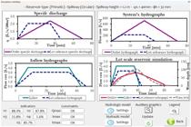
Figure 8
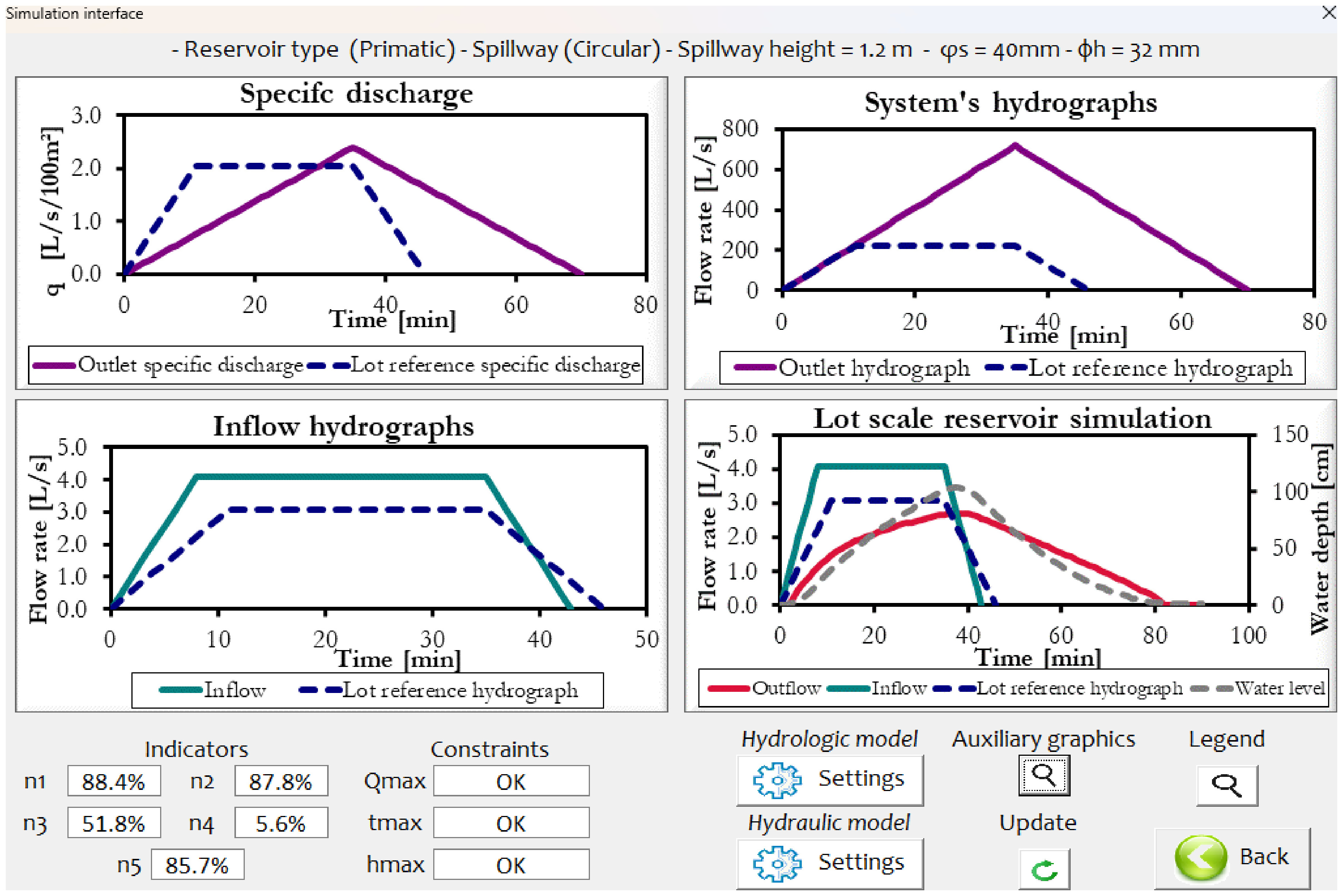
Simulation results of Example 1. At the top header, the current tested solution is indicated. The performance indicators are shown in the bottom left, and the model constraints of maximum outflow, minimum time to peak, and maximum water depth are satisfied in this example. In the tool, users can also adjust hydrologic and hydraulic parameters and visualize PULS auxiliary graphics to solve the mass balance equations.
Figure 9
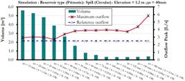
Outlet orifice diameter Monte-Carlo analysis, where all feasible internal diameters are tested to identify the minimum volume that attends the maximum flow discharge and peak time constraints.
Figure 10
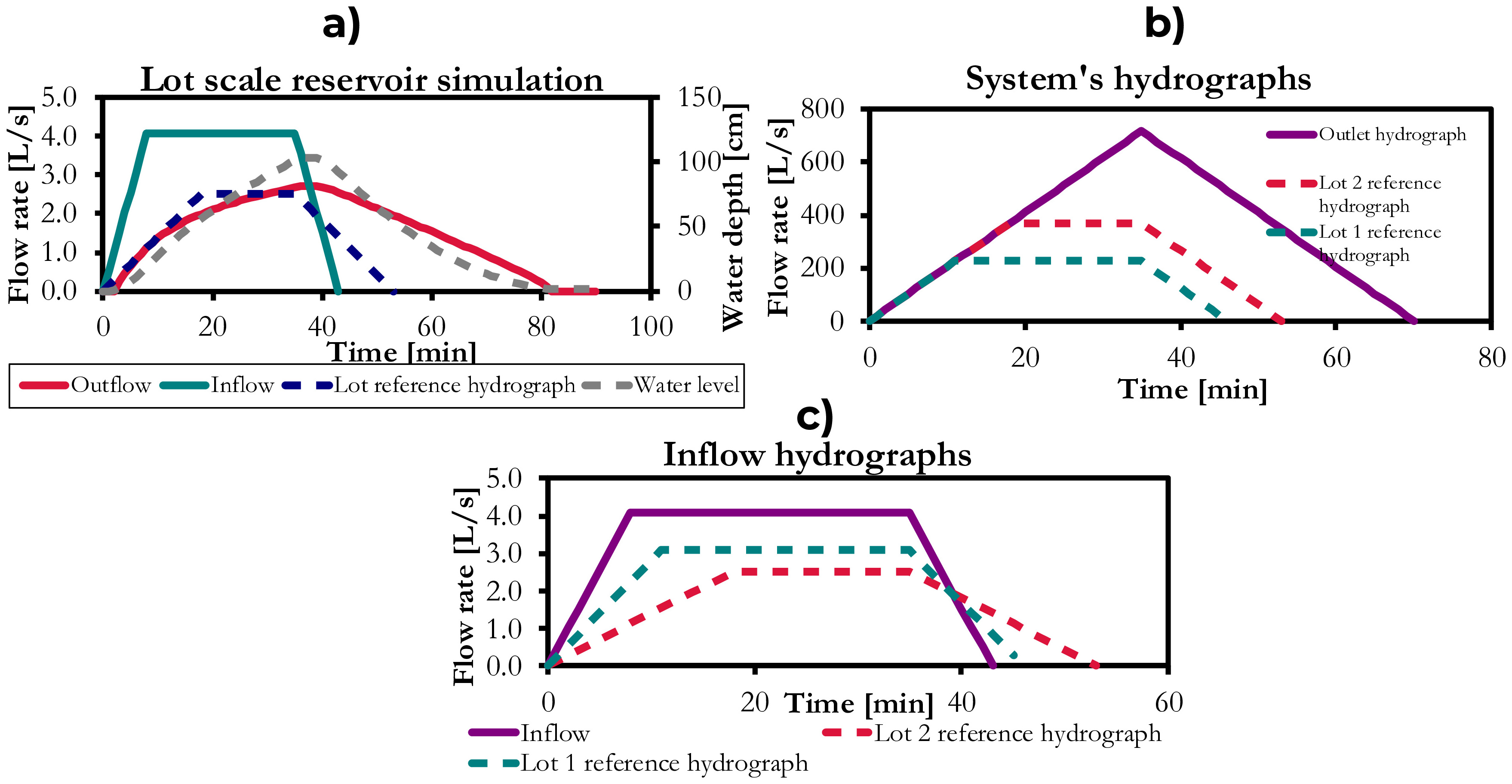
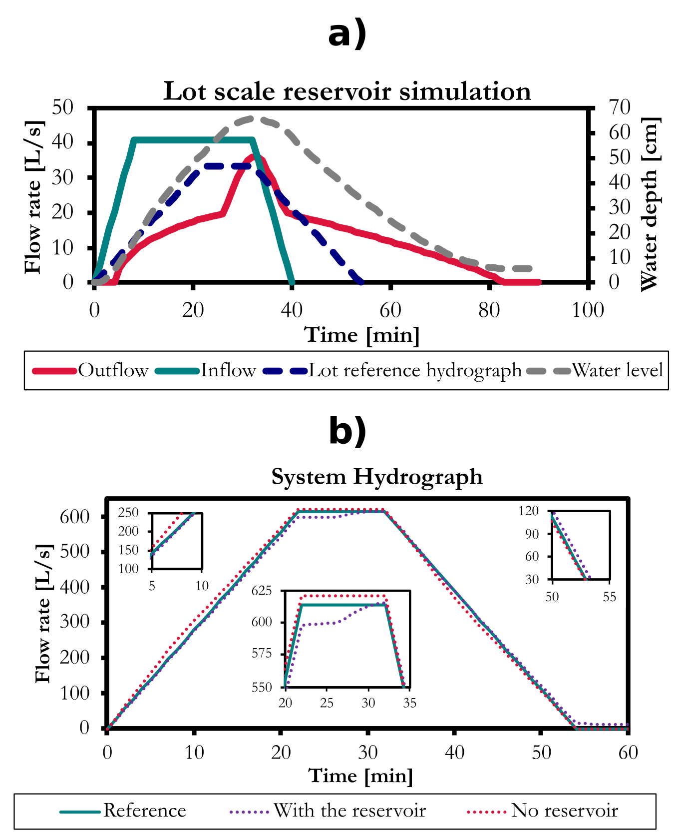
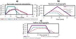
(a) Inflow, outflow, and water level in the reservoir for Example 1 results, (b) System’s hydrographs, and (c) Inflow and reference hydrographs for lots 1 and 2.
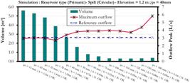
Figure 11
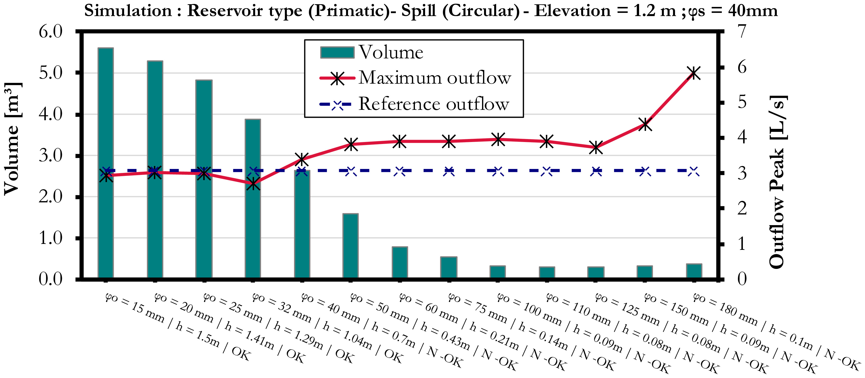
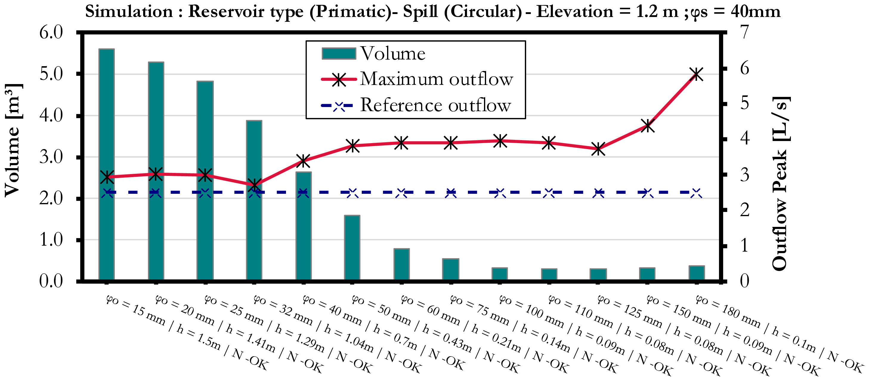
Lot’s 2 reservoir orifice assessment showing the performance of different orifice configurations for the same overall design of Example 1, which consisted of a circular spillway 1.2 m from the bottom with a 40 mm diameter and the reservoir with a 3.75 m.
Figure 12
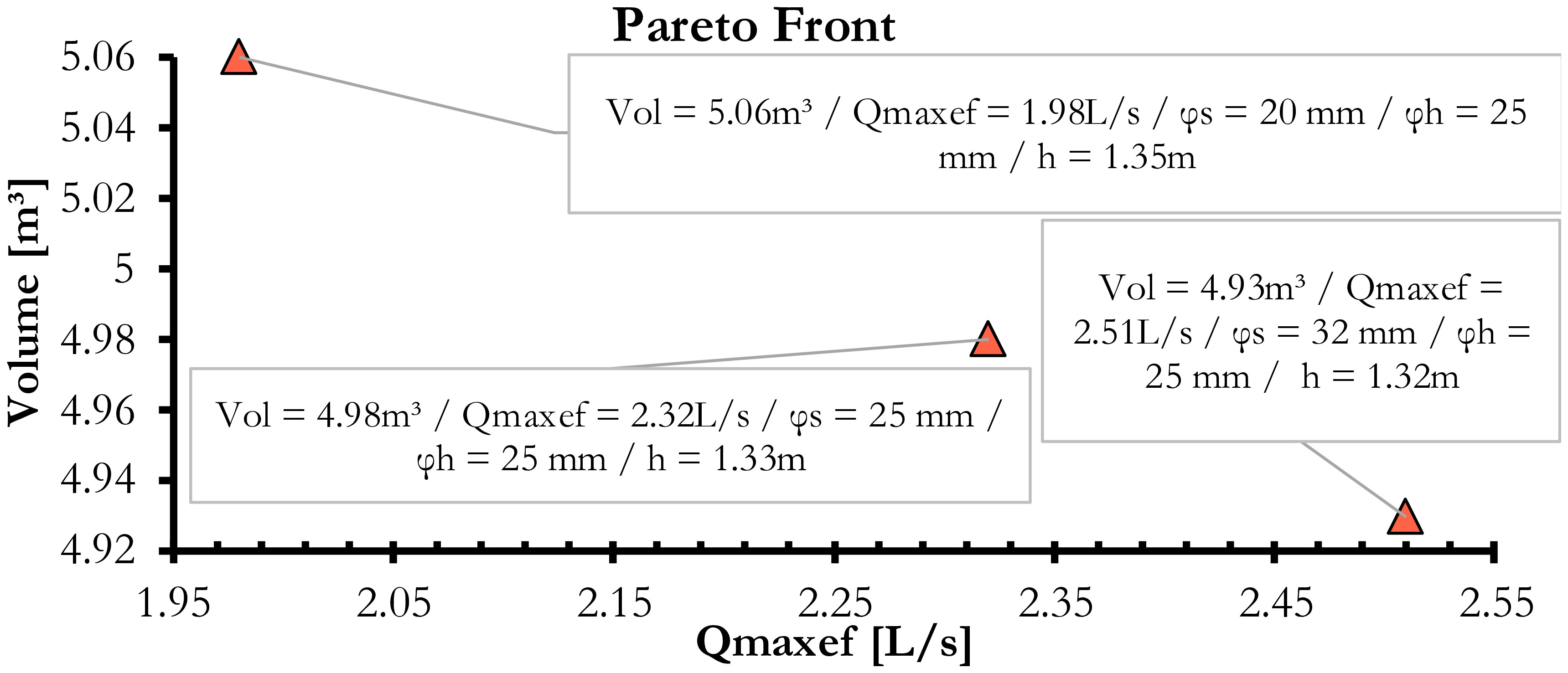
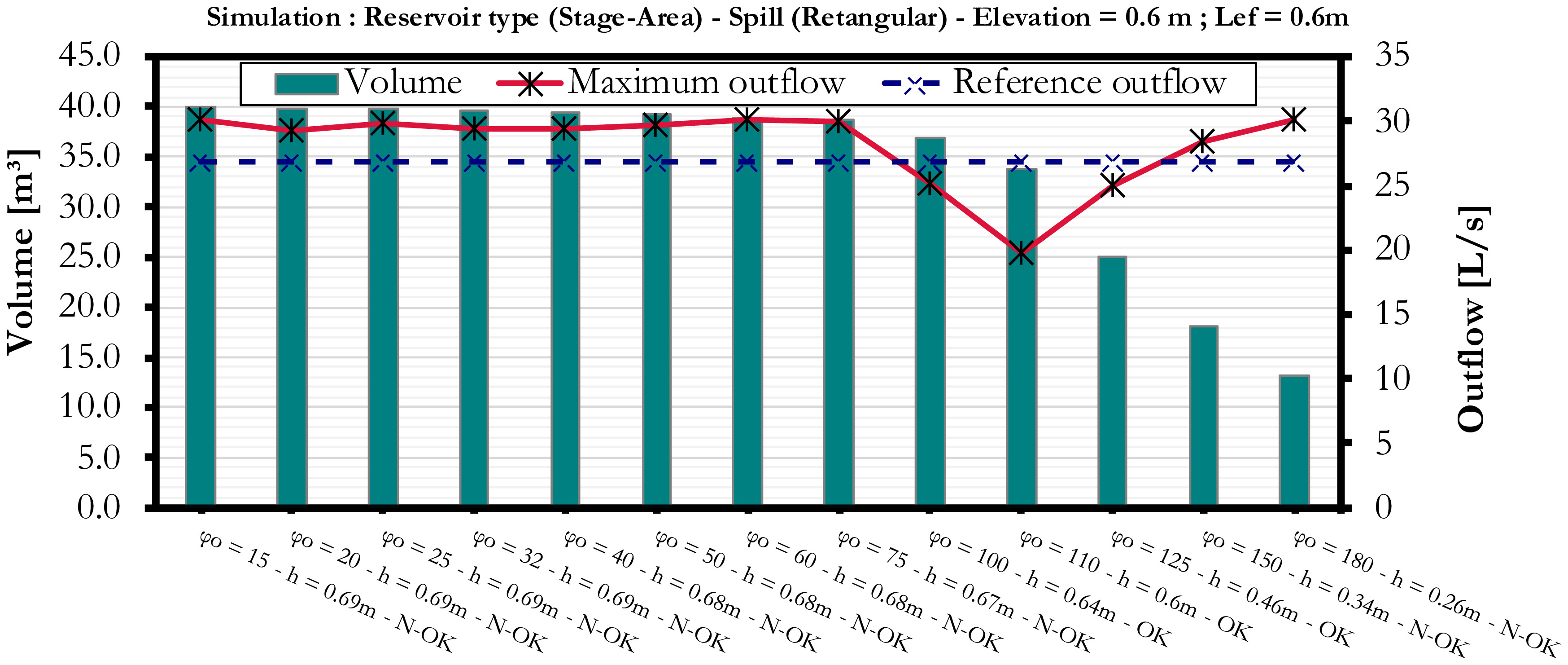
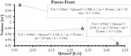
Pareto Front of non-dominated solutions when comparing reservoir volume with the maximum outflow.
Figure 13
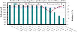
Orifice outflow assessment for example 3 – the micro detention pond – for a 10-yr storm event focusing on evaluating the orifice capacity while avoiding spillway flow.
Figure 14
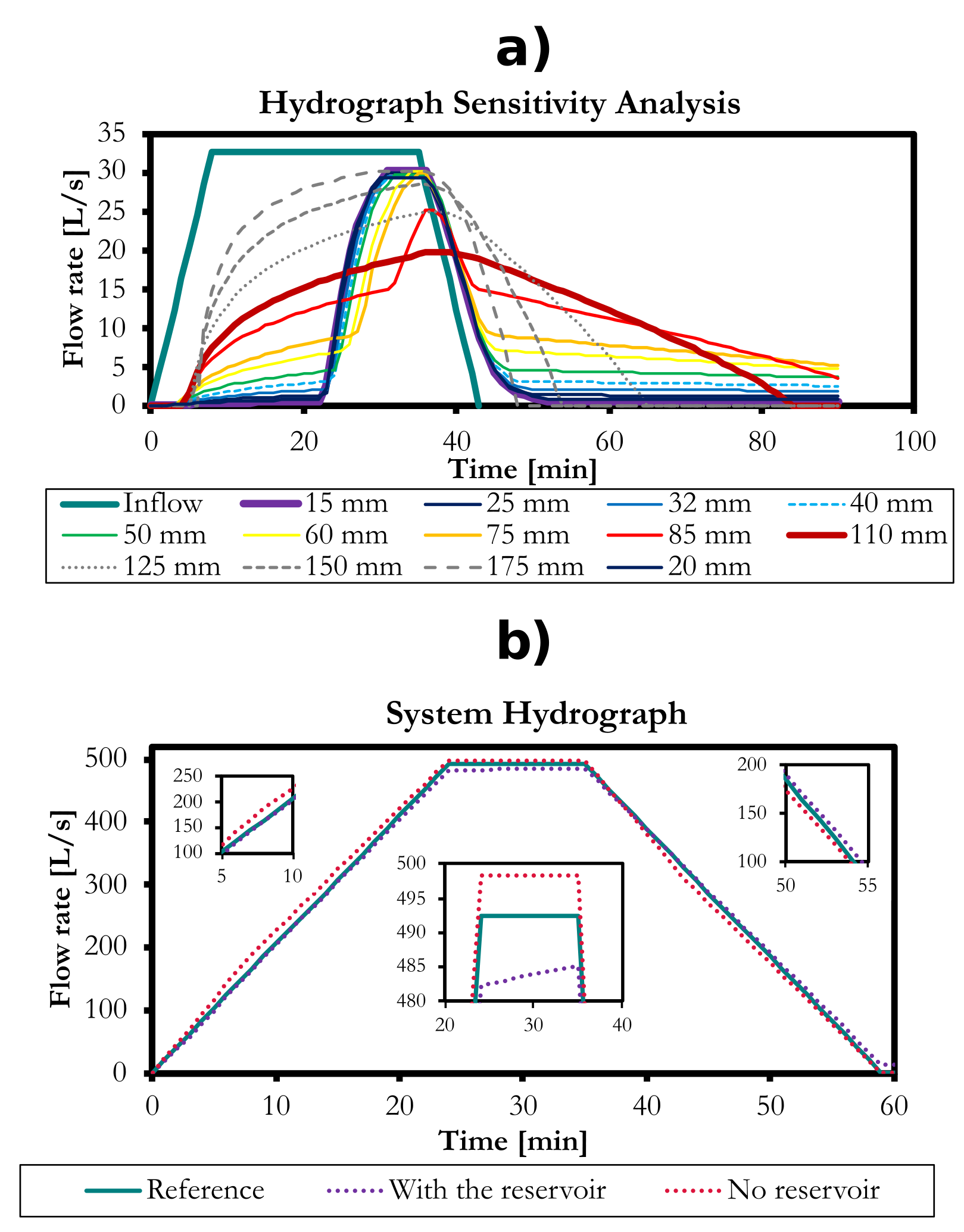
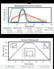
Outflow hydrograph sensitivity analysis where the 110 mm diameter is the optimal solution for the 10-yr design (a), and the effect of the reservoir dynamics on the lot reference hydrograph (b).
Figure 15
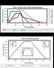
Hydrographs for a 25-yr-storm, where (a) shows the reservoir effects (it was designed for a 10-yr return period), whereas (b) shows the catchment-scale effect of the reservoir. Red dashed lines in (b) show the outlet hydrograph considering the waterproofing in the lot area without LID implementation.
Table 1
Performance indicators, where Vef is the cumulated outflow volume [L3], and Vp is the total rainfall volume over the catchment area [L3]. Variable tc,ef indicates the reservoir effluent time of concentration, and Qmaxef the reservoir effluent peak flow.
Table 2
Hydrologic results for example 2.
Table 3
Comparison between reservoirs of example 1 and 2, where Vol represents the minimum volume.
Table 4
Hydrologic model results for example 3 for the 10-yr and 25-yr storms. Note that, unlike empirical geometry-based time of concentration formulations, the time of concentration decreased with the increase in return period.

 Consideração da variabilidade espacial do escoamento superficial no projeto de LID para bacias urbanas: desenvolvimento de modelo e software
 Thumbnail
 Thumbnail
 Thumbnail
 Thumbnail
 Thumbnail
 Thumbnail
 Thumbnail
 Thumbnail
 Thumbnail
 Thumbnail
 Thumbnail
 Thumbnail
 Thumbnail
 Thumbnail
 Thumbnail