Scenario reduction using machine learning techniques applied to conditional geostatistical simulation

Abstract

One of the basic factors in mine operational optimization is knowledge regarding mineral deposit features, which allows to predict its behavior. This could be achieved by conditional geostatistical simulation, which allows to evaluate deposit variability (uncertainty band) and its impacts on project economics. However, a large number of realizations could be computationally expensive when applied in a transfer function. The transfer function that was used in this study was the NPV net present value. Hence, there arises a necessity to reduce the number of realizations obtained by conditional geostatistical simulation in order to make the process more dynamic and yet maintain the uncertainty band. This study made use of machine-learning techniques, such as multidimensional scaling and hierarchical cluster analysis to reduce the number of realizations, based on the Euclidean distance between simulation grids. This approach was tested, generating 100 realizations by the sequential Gaussian simulation method in a database. Proving that similar uncertainty analysis results can be obtained from a smaller number of simulations previously selected by the methodology described in this study, when compared to all simulations.

keywords:
geostatistical simulation; scenario reduction; machine learning; net present value (NPV)

1. Introduction

The minerals used by mankind come from deposits scattered around the world, and just as always, commodity prices are defined by world supply and demand. Thus, for the mineral to be considered as ore, it depends on the costs that will be applied in the planning, implementation and production phases. In order to turn an enterprise into a profitable one, in a long-term perspective, planners must continually examine and evaluate more efficient and specific methods to streamline processes and reduce costs. To do so, it is necessary to know and understand the deposits's behavior, in addition to mastering the tools / techniques used in estimation and mining processes. Cost savings through efficient and environmentally sustainable mining practices are and will be even more important in the future because of increasing underground mining depths and increasingly stringent regulations (HUSTRULID; KUCHTA; MARTIN, 2013).

Monkhouse and Yeates (2018) define the practice currently employed in the mine planning industry as deterministic; that is, done considering a single estimate, generated by using a unique set of mining assumptions along with pre-defined external economic factors to create a mathematical optimized pit, which will be used as references for subsequent optimization processes, such as mine scheduling. Among the most used and known interpolation algorithms are: kriging, polygons, inverse square distance among others. The optimization process can be applied to several mining variables. However it is most commonly used in Net Present Value (NPV) evaluation, which is the difference between the present value of the cash inflows and the present value of the outputs in a period of time. NPV is used in the capital budget to analyze the profitability of an investment or project.

One of the interpolation algorithm characteristics is the tendency to smooth the local spatial variation details of the attribute of interest being modeled (usually grades), which constitutes a method disadvantage especially in cases with high variation coefficient deposits. Normally, small values are overestimated, while large values are underestimated. In addition, another aggravating factor is the fact that smoothing is not uniform because it is dependent on local data configuration: smoothing is minimal near the places where there is data and increases where the estimated location has little data. The results of kriging could be more variable in densely sampled areas than in poorly sampled ones, thefore may exhibit undesirable artifacts (GOOVAERTS, 1997).

A key factor to understand, and even to predict the deposit's grade behavior is to know the uncertainty associated with it. Uncertainty measurement is performed using simulations and comparison of the value range obtained at the same location. This type of uncertainty is measured generating multiple realizations of the variable value's joint distribution in space. This process is known as stochastic simulation (GOOVAERTS, 1997).

Stochastic simulation provides a way to incorporate various types of uncertainty into the prediction of a complex system response. Usually, some information is available in a parameter of interest, but the transfer function (a groundwater flow model, for example) may require a detailed spatial mapping of this parameter. The exhaustive sampling required to obtain this map is generally not feasible. An alternative is to generate realizations from a random field that shares the information available in the parameter of interest. These outputs serve as input to a transfer function that calculates a system response for each simulation. If the performances characterize the spatial uncertainty of the parameter of interest, the resulting value distribution of the expected system response will reflect this uncertainty (ARMSTROG; DOWN, 2013).

Goovaerts (1997) makes a comparison between kriging and conditional geostatistical simulation, and Journel (1974) states that maps generated by interpolation (kriging) provide a single value when applied to a transfer function; in the case of this article, the NPV. On the other hand, with the conditional geostatistical simulation, it is possible to generate several realizations that respect mineral deposit statistical characteristics, such as histograms and spatial continuity, besides honoring the sampling points. The set of generated outputs provides a visual and quantitative measure (indeed, a model) of spatial uncertainty.

Stochastic spatial simulations are widely used to generate multiple and equiprovable realizations of a spatial process and to evaluate related uncertainties. Uncertainty is the result of our lack of knowledge of the mineral deposit. Therefore, it is an inherent characteristic of geological models. This stems essentially from the fact that it is impossible to characterize the true distribution of the studied property among the data sets. Thus, uncertainty is not an attribute of the studied process itself and, unlike error, cannot be measured in an absolute way (JAKAB, 2016).

Although currently computational technology allows an increased number of geostatistical simulation realizations, in addition to automating it, human inspection is still required to control and analyze the results and its validations. However, post-processing capability for a transfer function (NPV) did not accompany the ability to create the outputs. Processing and analyzing large numbers of outputs in a qualitative and productive way is quite costly even in computational terms. It is difficult to recognize and understand the variations that occur between multiple realizations generated by geostatistical simulation methods. Generally, only a few outputs are displayed and analyzed satisfactorily (ARMSTRONG et al., 2014).

Several challenges need to be addressed when considering reduction of the number of simulation realizations to obtain a minimum number of outputs which characterizes the uncertainty band in the same way, i.e. that are enough to describe the variable's behavior. The first challenge is to define a distance measure between pairs of realizations. This measurement distance is specifically developed for mining, although it may be also suitable for other applications. The second challenge is to improve the procedure for selecting a subset of the exhaustive set of available simulated realizations (ARMSTROG et al., 2013). This subset must satisfactorily aproximate the uncertainty of the NPVs dispersion.

Multidimensional scheduling is a good method to explain these three basic steps. In the first step, a range of distances between all pairs of data is obtained. The second step involves estimating an additive constant and using this estimate to convert the comparative distances to absolute distances. In the third step, the dimensionality of the space needed to explain these absolute distances is determined, and data projections in the axes of that space are obtained (Torgerson, 1952).

Multidimensional Scaling (MDS) has become popular as a technique for analyzing multivariate data. MDS is a method for dimensionality reduction analysis. MDS results in measurements of similarity or dissimilarity of input data under investigation. The primary result of an MDS analysis is a 2D plot\. This new spatial configuration has a lower dimension than the original space. The points in this spatial representation are organized in such a way that their distances correspond to the similarities of objects: similar objects are represented by points close to each other, different objects by distant points (WICKELMAIER, 2003).

Hierarchical cluster analysis (HCA) is a method which seeks to build a hierarchy of clusters, one by one, until clustering all points in a single group. One of the HCA features is to display the data in a two-dimensional space in order to display the groupings, the dendrogram. The distance between the points reflects the similarity of its properties, being useful to determine the similarity between objects. The method relates samples in a way that the most similar are grouped together. The results are presented as a dendrogram, in which it groups the objects in function of similarity (KOHN; HUBERT, 2006).

Thus, this article aims to investigate machine learning techniques (MDS and HCA) to select representative realizations, i.e. reduction in order to calculate economic value (NPV). The goal is to reduce the number of realizations to be postprocessed, maintaining the representativity of the exhaustive set of realizations, ensuring greater agility and lower computational costs. The MDS and HCA techniques were used for this purpose.

Scenery reduction approach

In the reduction stage scenario, the size of the final subset is determined by the user at the beginning of the process. This subset corresponds to the maximum number of outputs that can be conveniently postprocessed. To illustrate the problem, in the case of petroleum deposits, post-processing involves fluid flow simulation using specialized software, while in mining it corresponds to NPV optimization.

The three main components of any reduction method scenario applied to geostatistical simulations are: (i) to define the distance between two simulated realizations. This depends on the goal of the study. In mining, a better knowledge of the mineral deposit or quantification of the uncertainties associated with it can lead to risk reduction, while in the oil industry, the fluid flow properties are crucial; (ii) define the metric to measure similarity / dissimilarity between all pairs of realizations; and (iii) select the algorithm that generates the best subset of predetermined number of simulation at the end.

2. Material and methods

Making use of a two-dimensional synthetic database containing the variable Copper (Cu), the Walker Lake database (ISAAKS; SRIVASTAVA, 1989), the geological uncertainty model was built using the variable Cu with a determined number of equiprovable scenarios, with the geostatistical simulation technique. A hundred simulated scenarios were generated using the Gaussian sequential simulation methodology. After the methodology was carried out, the necessary checks of reproducibility of first and second order and of accuracy were made. It was verified that the results were satisfactory in the reproducibility of the spatial phenomenon.

The simulations where divided into pairs and, each pair of realizations received a similarity value. Armstrong et al. (2013) used as a measure of similarity, the amount of metal in each panel above a set of 16 cut-off points. Another possible option would be to use both tonnage or metal content above the cutoff point. Defined the distance measurement method between pairs of realizations, a distance matrix B of size N × N is constructed, where N is the total number of realizations. Once the distance matrix B was built, the realizations will be mapped into a smaller dimension Euclidean space using multidimensional scaling (MDS). As result from comparison between realizations, the smaller the values the more similar are the realizations, and the larger, the more distinct.

The next step consists of Hierarchical Cluster Analyzes (HCA), where each object is initially considered as a single-element group. At each step of the algorithm, the two most similar groups are combined into a new larger group. This procedure is iterated until all points are members of only a single large group. The result is a tree that can be plotted as a dendrogram. In this way, it is possible to select as many roots as necessary according to the user's demands. In this study, the number chosen was ten; that is, the total number of realizarions was divided into 10 groups (not necessarily of the same size), and from each group a representative realization of the respective group was chosen.

To select one realization per group, a Python language script was built, which measures the distance of one point against all others in the same group. This process is repeated for all points in the same group. Thus, the point that has the lowest distances sum will be the one chosen to represent its group. Initially, the idea was do the same step of Armstrong et al. (2013). However, there have been cases where more than one point was given as optimal, and as only one can be selected per group, the technique mentioned above was developed.

After selecting the 10 representative realizations, a profit function was applied to assign economic values to the blocks in all realizations. The NPV values of the selected realizations using the proposed methodology were compared with the NPV values of the exhaustive simulation. In this way, it was possible to verify if the proposed methodology satisfactorily reproduced the simulation statistics.

In this study, used was NPV as the transference function, and according to the mine scheduling, all 3120 blocks will be mined along the y direction, starting at the northern end of the deposit and advanceing from left to right.

To calculate the NPV for all realizations, an economic value is assigned for all blocks of each realization, using the copper grade of each block. Equation 1 shows the logical procedure used.

(1) $\mathit{evb}=\left\{\begin{array}{c}\left\{\left[\left(\frac{\mathit{Cu}\%}{100}\right)\times \left(\mathit{rec}\right)\times \left(\mathit{sp}-\mathit{rc}\right)\right]-\left[\mathit{mc}-\mathit{bc}\right]\right\}\times \mathit{bm}\mathit{if}\mathit{evb}>-\left(\mathit{mc}\times \mathit{bm}\right)\hfill \\ -\left(\mathit{mc}\times \mathit{bm}\right)\mathit{otherwise}\hfill \end{array}\right.$

• evb - economic value of the block (US $);

• Cu% - grade (%) of copper for the block;

• rec - metal recoveringmetal during mining and processing (until the end of the concentration stage) = 94%;

• sp - long-term sales price per ton of metal = US $ 5600 / t;

• rc - refining cost per ton of metal = US $ 200 / t;

• mc - mining cost (outsourced) per ton of ore = US $ 2.98 / t;

• bc - beneficiation cost per ton of ore = US $ 6.5 / t;

• bm - block mass = 62.5 t, considering the density of all blocks equal to 2.5 t / m³.

The values used in equation 2 were updated to today's values, obtained from an active copper mining.

3. Results and discussion

Since post-processing of all realizations is time consuming, it has been defined that the realizations subset must contain a number that representes 10% of the total generated by the simulation. Since these tests were run with a set containing one hundred realizations, while the generated subsets contain 10 realizations.

One hundred realizations were generated by the Gaussian sequential simulation method (SGSim) in point support. After the production and validation of the simulation, a support change from points to blocks with dimensions of 5 x 5 x 1 m (x, y and z respectively) was made. The dimensions of the final grid are 60 blocks in the North-South direction, 52 in the East-West direction.

To generate the distance matrix all pairs of grids (block support) were compared according to Equation 2.

(2) $\mathit{D}\left({\mathit{G}}_1,{\mathit{G}}_2\right)=\frac{{\sum }_{i=\mathit{1}}^{\mathit{N}}\mathrm{abs}\left({\mathit{G}}_{1}i,{\mathit{G}}_{2}i\right)}{\mathit{N}}$

Where D is the distance between pairs of grids, G are the grids, N is the number of blocks in each grid and i is the grid block under study.

A 100x100 transposed matrix was constructed containing the distances of each pair of grids. Through the script described above, the distance matrix is incorporated into a two-dimensional map using the sklearn.manifold.MDS (Pedregosa et al., 2011) library (Figure 1).

Figure 1
MDS graph with non defined groups.

With the same Python script, the realizations, which after the MDS incorporation are in the form of points, were grouped in 10 sets represented in a dendogram (Jones et al., 2001). This was performed with the HCA technique looking for homogeneous clustered items represented by points in an n-dimensional space in 10 groups, relating them with similarity coefficients. The number of points in each group ranges from 6 to 14 realizations, since regions in space that are more densely occupied will have a greater number of realizations than those with sparse occupation.

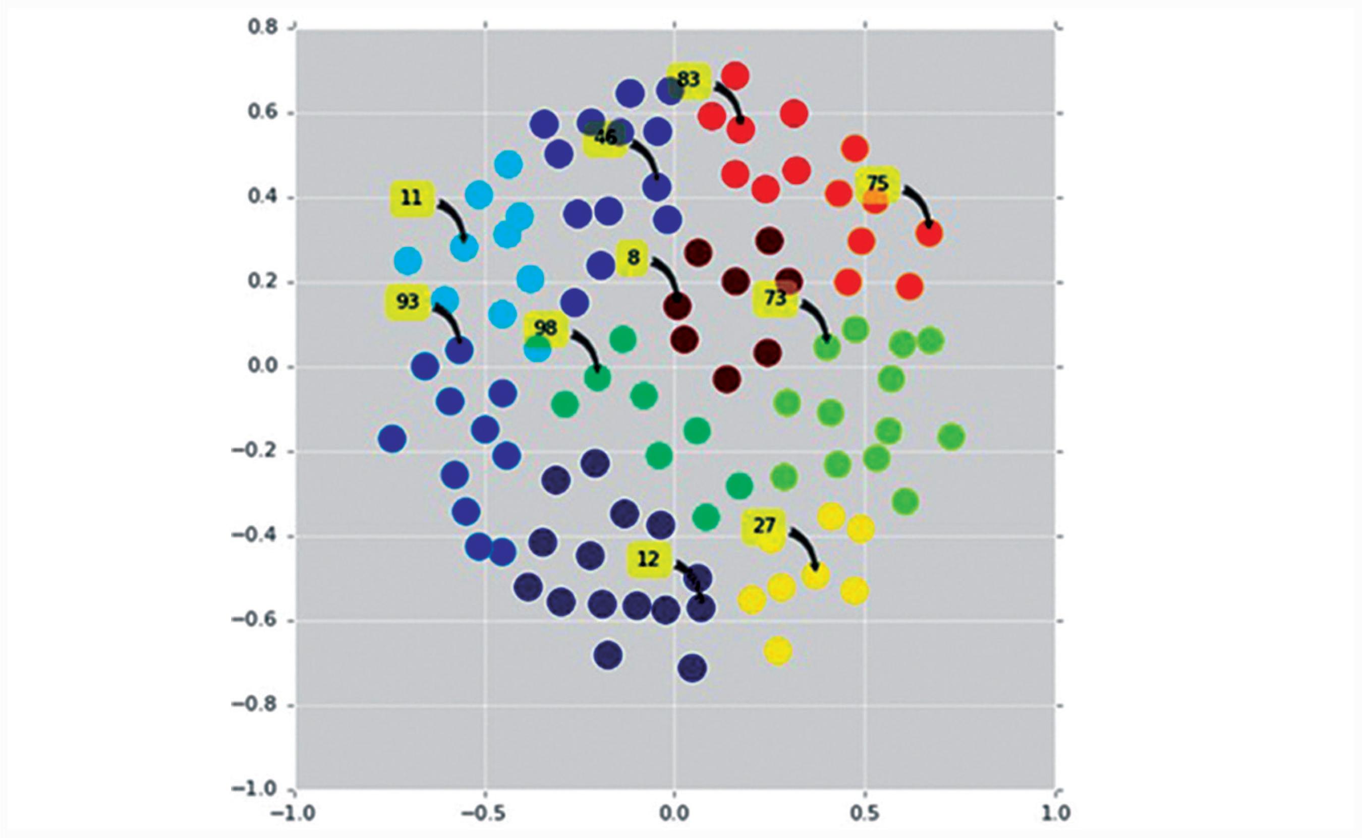
After the realization cluster, one realization (the most representative of each group) was selected using script in python programming language. The selection of a realization from each group was performed with the distance sum of a realization to all others in the same group. The realization with the lowest sum resultant value was chosen according to the stability theory. Figure 2 below shows the realization grouping in the 10 different clusters (each color represents a cluster) and indicates the number of the selected realization to represent each group.

Figure 2
MDS graph separating each cluster of realization by color. Most representative realizations, from each cluster, are indicated by arrows along with their respective numbers.

For each block of each realization, a profit function was applied to obtain its economic value and proceed with the NPV evaluation.

Table 1 shows the maximum and minimum NPV values, the difference between the maximum and minimum, and the amplitude that this difference represents. These values were calculated for the following situations: all 100 realizations; the 10 realizations selected with the method developed in this work; the mean of the maximums and minimums of 10 randomly chosen realizations 50 times; and for 10 randomly selected realizations from the clustering method (HCAR) used in this work, that is, selected without taking into account the sum of the distances. There are interesting parallels with standard practice in the oil industry, selecting only three realizations: the P10, P50 and P90 realizations. As the average does not interest at this moment, only 2 realizations, P10 and P90 (chosen from the amount of metal above the cut-off point) were selected.

Table 1
Resultant values for each scenario evaluated (methods) with maximum, minimum, number of scenarios used by each methodology, difference and their representativeness in relation to the base scenario (all realizations). (Amounts in US dollars).

NPV
	Number of simulations	Maximum	Minimum	Difference	Uncertainty band
Simulation	100	$ 32,125,674	$ 25,904,490	$ 6,221,184	100,00%
Scenario Reduction	10	$ 32,125,674	$ 26,586,308	$ 5,539,366	89,04%
Random (50x)	10	$ 30,907,346	$ 27,108,542	$ 3,798,704	61,06%
P10/P90	10	$ 30,678,148	$ 27,557,455	$ 3,120,693	50,16%
HCAR (50x)	10	$ 31,534,771	$ 27,529,480	$ 4.005,291	64,38%

The analysis evaluating all 100 realizations (exhaustive case), was considered as the base case for comparison with the other evaluated methods, considering that this case provides the best and the worst case. After applying the profit function and NPV calculation, the minimum and maximum values obtained are US$ 25,904,490 and US$ 32,125,674, respectively.

In the scenario of ten realizations selected from the methodology developed in this study, the minimum and maximum values were very similar to those obtained in the base case, corresponding to 89.04% of its uncertainty band, which indicates good representativeness of the exhaustive case

The three other evaluated cases were less representative, with better results obtained by the HCAR method, reproducing a 64.38% of uncertainty band. These results demonstrate that selecting 10 realizations with the method of distances between realizations is quite efficient, considering that it satisfactorily reproduced the variability of the exhaustive case with a lower computational cost.

The database used in this study is not extensive, and the processing time is small both in the exhaustive case and in the cases with selection of 10 realizations, making it difficult to detect the benefit of the selection. However, in extensive databases, the benefit will be apparent, making simulated post-processing much faster and more dynamic.

4. Conclusions

This article proposed a method for selecting a representative subset of geostatically simulated realizations of a mineral deposit from a larger set, based on the reduction method scenario developed in the field of stochastic optimization. Three main parameters were vital in the process of selecting representative subsets of realizations:

1. The distance between two realizations (or scenarios);

2. The metric to measure the similarity / dissimilarity between the simulated set (or scenarios) and a subset of their realizations;

3. The algorithm used to find the "best" subset.

The approach used as a basis to develop the methodology presented herein, proposes a new way of measuring the distance between pairs of geostatistical realizations, focused on mining, through usage of the distance between grids. The innovation in this study relies on the development and use of a non-random search algorithm to find a representative realization subset of the total set of realizations, allowing greater agility in the post-processing of simulated models.

The proposed method was tested in a synthetic copper database. Using only 10 selected realizations, from a universe of 100, it was possible to obtain very similar and representative results of the exhaustive case (approximately 90% of the uncertainty band). This result demonstrates the efficiency of the proposed method, which is representative of the simulation as a whole, but at a much lower computational cost.

Acknowledgments

The authors would like to thank the colleagues and professors of the Laboratory of Mineral Research and Mining Planning (LPM - UFRGS) who have greatly assisted this work.

References

• ARMSTRONG, M., DOWD, P. (2013) Geostatistical simulations. Proceedings of the Geostatistical Simulation Workshop, Fontainebleau, France, 27-28 May 1993. [S.l.]: Springer Science & Business Media, 2013. v. 7.
• ARMSTRONG, M. et al. Scenario reduction applied to geostatistical simulations. Mathematical Geosciences, Springer, v. 45, n. 2, 2013. p. 165-182.
• ARMSTRONG, M. et al. Genetic algorithms and scenario reduction. Journal of the Southern African Institute of Mining and Metallurgy. The Southern African Institute of Mining and Metallurgy, v. 114, n. 3, p. 237-244, 2014.
• GOOVAERTS, P. Geostatistics for natural resources evaluation [S.l.]: Oxford University Press on Demand, 1997. 483 pp.
• HUSTRULID, W. A., KUCHTA, M., MARTIN, R. K. Open pit mine planning and design (Two volume set & CD-ROM pack). CRC Press, 2013.
• ISAAK, S., SRIVASTAVA, R. Applied geostatistical series New York: Oxford University Press, 1989. 561p.
• JAKAB, N. Uncertainty assessment based on scenarios derived from static connectivity metrics. Open Geosciences, De Gruyter Open, v. 8, n. 1, p. 799-807, 2016.
• JONES, E. et al. SciPy: Open source scientific tools for Python. 2001-. Disponível em:, <www.scipy.org>.
  » www.scipy.org
• JOURNEL, A. G. Geostatistics for conditional simulation of ore bodies. Economic Geology, Society of Economic Geologists, v. 69, n. 5, p. 673-687, 1974.
• KÖHN, H.-F., HUBERT, L. J. Hierarchical cluster analysis Wiley StatsRef: Statistics Reference Online, Wiley Online Library, 2006
• MONKHOUSE, P., YEATES, G. Beyond. naive optimisation. In: Advances in Applied Strategic Mine Planning [S.l.]: Springer. 2018. p. 3-18.
• PEDREGOSA, F. et al. Scikit-learn: machine learning in Python. Journal of Machine Learning Research, v. 12, p. 2825-2830, 2011.
• TORGERSON, W. S. Multidimensional scaling: I. theory and method. Psychometrika, Springer, v. 17, n. 4, p. 401-419, 1952.
• WICKELMAIER, F. An introduction to mds. sound quality research unit. Denmark, Citeseer: Aalborg University, 2003. v. 46, n. 5.

Publication Dates

• Publication in this collection
  Jan-Mar 2019

History

• Received
  06 Sept 2018
• Accepted
  13 Dec 2018