Abstract
In the context of multi-environment trials, where a series of experiments is conducted across different environmental conditions, the analysis of the structure of genotype-by-environment interaction is an important topic. This paper presents a generalization of the joint regression analysis for the cases where the response (e.g. yield) is not linear across environments and can be written as a second (or higher) order polynomial or another non-linear function. After identifying the common form regression function for all genotypes, we propose a selection procedure based on the adaptation of two tests: (i) a test for parallelism of regression curves; and (ii) a test of coincidence for those regressions. When the hypothesis of parallelism is rejected, subgroups of genotypes where the responses are parallel (or coincident) should be identified. The use of the Scheffé multiple comparison method for regression coefficients in second-order polynomials allows to group the genotypes in two types of groups: one with upward-facing concavity (i.e. potential yield growth), and the other with downward-facing concavity (i.e. the yield approaches saturation). Theoretical results for genotype comparison and genotype selection are illustrated with an example of yield from a non-orthogonal series of experiments with winter rye (Secalecereale L.). We have deleted 10 % of that data at random to show that our meteorology is fully applicable to incomplete data sets, often observed in multi-environment trials.
Scheffé multiple comparison method; joint regression analysis; test for parallelism; test of coincidence
BIOMETRY, MODELING AND STATISTICS
Analyzing genotype-by-environment interaction using curvilinear regression
Dulce Gamito Santinhos PereiraI,* * Corresponding author < dgsp@uevora.pt> ; Paulo Canas RodriguesII,IV; Iwona MejzaIII; Stanislaw MejzaIII; João Tiago MexiaII
IUniversidade de Évora/Escola de Ciências e Tecnologia CIMA-UE - Depto. de Matemática, R. Romão Ramalho, 59 - 7000-671 - Évora - Portugal
IIFCT/UNL - Centro de Matemática e Aplicações - 2829-516 - Caparica - Portugal
IIIPoznan University of Life Sciences - Dept. of Mathematical and Statistical Methods, ul. Wojska Polskiego 28 - 60-637 - Pozna - Poland
IVISLA Campus Lisboa, Laureate International Universities, Estrada da Correia, 53 - 1500-210 - Lisboa, Portugal
ABSTRACT
In the context of multi-environment trials, where a series of experiments is conducted across different environmental conditions, the analysis of the structure of genotype-by-environment interaction is an important topic. This paper presents a generalization of the joint regression analysis for the cases where the response (e.g. yield) is not linear across environments and can be written as a second (or higher) order polynomial or another non-linear function. After identifying the common form regression function for all genotypes, we propose a selection procedure based on the adaptation of two tests: (i) a test for parallelism of regression curves; and (ii) a test of coincidence for those regressions. When the hypothesis of parallelism is rejected, subgroups of genotypes where the responses are parallel (or coincident) should be identified. The use of the Scheffé multiple comparison method for regression coefficients in second-order polynomials allows to group the genotypes in two types of groups: one with upward-facing concavity (i.e. potential yield growth), and the other with downward-facing concavity (i.e. the yield approaches saturation). Theoretical results for genotype comparison and genotype selection are illustrated with an example of yield from a non-orthogonal series of experiments with winter rye (Secalecereale L.). We have deleted 10 % of that data at random to show that our meteorology is fully applicable to incomplete data sets, often observed in multi-environment trials.
Keywords: Scheffé multiple comparison method, joint regression analysis, test for parallelism, test of coincidence
Introduction
Farmers and scientists aim to identify superior performing genotypes across a wide range of environmental conditions. Here, by environments we mean combinations of locations and years. The main source of differences between genotypes in their yield stability is the fact that the genotype and environment effects are not additive, i.e. genotype-by-environment interaction (GEI) is present in the data. This interaction can be due to contrasting drought stress levels, winter low temperature stress, abiotic stresses, growing cycle duration, availability of nutrients, etc. The GEI can be expressed either as crossovers, when two different genotypes change in rank order of performance when evaluated in different environments, or inconsistent responses of some genotypes across environments without changes in rank order. The study and understanding of these interactions is a major challenge for breeders and agronomic researchers attempting to improve complex traits (e.g. yield) across environmental conditions.
Various techniques have been used to analyze the interaction in general and GEI in particular. Readers interested in those methods are referred to e.g. Aastveit and Mejza (1992); Annicchiarico (2002); Gauch (1992); Kang and Gauch (1996); Romagosa et al. (2009).
Regression is one of the most popular and most applicable methods used for inference about genotype comparison and selection in the context of multi-environmental experiments. In regression analysis two sets of variables are used, the first characterizing genotypes, and the second environments. The so-called adjusted means (or some other genotypic characteristic) for genotypes usually constitute observations of the dependent variable. In our illustration we take the original observations of the phenotypic variable as a realization of each dependent variable. The independent variable is defined by environmental indexes, which represent a measurement of productivity. Although Finlay and Wilkinson (1963) defined these environmental indexes as the average over all environments for every genotype, in this study we compute them with an iterative zigzag algorithm (Mexia et al., 1999; Pereira and Mexia, 2010) which leads to the best linear unbiased estimators of the joint regression parameters. In joint regression analysis (JRA), after selecting the variable of interest (e.g. yield), the joint regression model adjusts a linear regression per genotype across all environments (Pereira et al., 2011; Rodrigues et al., 2011), on a synthetic variable measuring productivity, the environmental index. Several variants of JRA have been proposed. The one in which we will be interested here was first proposed by Gusmão (1985), who showed that the precision in analyzing series of randomized block experiments was increased by considering environment indexes for individual blocks instead of only one environmental index per environment. Mexia et al. (1999) introduced the L2 environmental indexes obtained by minimizing the sum of sums of squares of residuals, both in order to the coefficients of the regressions and to the environmental indexes.
Here a generalization of the joint regression analysis is presented for cases where the response (e.g. the yield) is not linear across environments and can be written as a second (or higher) order polynomial or another non-linear function. In our considerations we shall start with the estimation of the regression functions (linear or curvilinear) independently for all genotypes. In the second step the hypothesis of parallelism of regressions for all genotypes is tested. In general it is expected that the hypothesis of parallel regression lines will be rejected because of the presence of GEI in the data. If we reject the parallelism of regression curves, the next step to investigate GEI is to try to find subgroups of genotypes with similar responses to different environmental conditions. The genotypes can then be divided into groups based on the Scheffé multiple comparison method for regression coefficients, i.e. the genotypes with similar behavior will be grouped together and the calculations performed for each group separately.
The methodology will be illustrated by using a data set for winter rye (Secalecereale L.) from multi-environment trials carried out in the years 1997 and 1998 in Słupia Wielka, Poland (52º13' N, 17º13' E).
Materials and Methods
The zigzag algorithm
For convenience, let us consider data arranged in a two-way array with I rows and b columns. Suppose Yij is a continuous response variate (e.g. yield) for genotype i in block j if present. The joint regression model discussed here is an extension of that of Finlay and Wilkinson (1963) where the environmental indexes are computed for each block instead of for each environment. Assuming that the yield vectors are independent, normal, homoscedastic and that genotype i is present in block j (or replicate), the joint regression model can be written as:

with αi the intercept and βi the slope for genotype i, χj the block environmental index and εij the residuals. These environmental indexes represent the averages over a block/superblock and can be seen as a (spatial) measure of productivity.
Gusmão (1985, 1986) showed that the precision in analyzing series of randomized block experiments was improved considering environmental indexes for individual blocks of only one environmental index per experiment instead of one environmental index per environment. This proposal results in K experiments each with b blocks, i.e. Kb supporting points per regression instead of only K such points used by the classical Finlay-Wilkinson joint regression model (Finlay and Wilkinson, 1963).
To estimate the model parameters, we wish to minimize

where pij is the weight of genotype i in block j. If the genotype is absent we take pij= 0 . When the genotype occurs we take , j = 1, 2,..., b. These weights may differ from block to block to express differences in the representativeness of the blocks. If there are several blocks in the same location, their weights will be the same. In the illustration presented in this paper we use 1 and 0 for the weights, because no information was available about the relevance of the importance of blocks.
The zigzag algorithm (Pereira and Mexia, 2010) is used to minimize the loss function (2) iteratively, with respect to αi , to βi and to the environmental index χ j. For the complete case (i.e. all the genotypes are present in each environment) the average yield per block can be a good initial value for searching the environmental indexes (Gusmão, 1985). When incomplete blocks are used one may take the average yields for the corresponding superblock as the initial values. In the worst case any initial values may be taken, since the computation time does not increase much.
We assume that the yield vectors have components normally and independently distributed, so that the zigzag algorithm will lead to maximum likelihood estimators and enable us to make inferences while comparing genotypes.
The zigzag algorithm may be described as follows:
(i) Calculate the initial values for the environmental indexes
, which range within the interval [a0,b0], where and α0 = Min{χ01,...,χ0b} and b0 = Max {χ01,...,χ0b};
(ii) Minimize the function S(αJ, βJ|
and
;
(iii) To minimize S( xb|
(iv)
, j = 1, 2,..., b,
to obtain the new vector
(v) Standardize the vector of environmental indexes to keep the range unchanged. With
= Min{χ'01,...,χ'0b},
= Max {χ'01,...,χ'0b} take
; to obtain the vector,
, the new environmental indexes.
Repeat steps (ii) to (iv) until successive sums of sums of squares of weighted residuals differ by less than a fixed value.
At the end of each iteration, a standardization of the adjusted environmental indexes is carried out so that the range does not change from iteration to iteration. The procedure is carried out until the goal function stabilizes. The environmental indexes adjusted in this way are called L2 environmental indexes, because the L2 norm was used. The described zigzag algorithm is a version of the iterative algorithms existing in the literature; see for example, Digby (1979); Gabriel and Zamir (1979) and Ng and Williams (2001). Pereira and Mexia (2010) proved the convergence of the zigzag algorithm and that the adjusted parameters could be seen as maximum likelihood estimators. The alternative algorithms only considered the numerical adjustment.
Test for coincidence
Considering as before Yij, the phenotypic observation for genotype i in block j, j = 1,...,b; i = 1,..., I, and Xj, the environmental index for environment j, can be written as

where βik (k = 0, 1,..., t) are the t+1 unknown regression coefficients, zkj (=fk(xj)) are known functions of the environmental indexes xj, eij are independent and identically distributed random variables following normal distribution with E(eij) = 0, for all i, j, and

After identifying the regression functions for all genotypes, a test of coincidence for regressions can be used to check whether the yield responses for genotypes are similar with respect to environmental indexes. This test can be performed in two stages (Kleinbaum et al., 2008; Williams, 1967): (i) a test for parallelism of regression curves; and (ii) a test of coincidence for those regressions.
Equation (3) can be rewritten as

After centering the observations we have

The null hypothesis to test the parallelism of regression functions can be written as

where βck denotes the common kth regression coefficient, equal for all genotypes.
Let us consider now the case when some of the observations Yij are missing. Then, let ni (< b) be the number of environments in which the genotype i is observed, and  .
.
Classical regression techniques are used to estimate the parameters by the least squares method, independently for each genotype. Then we have

where bi is the vector of estimators of regression parameters for the genotype i, Zi is an (ni x t) matrix of centered values of explanatory variables, Yi = [Yi1, Yi2, ..., Yini]', i = 1, 2, ..., I. The SSi,e has ni - t - 1 degrees of freedom.
Table 1 gives the analysis of variance to test the parallelism of regression functions. The statistic FC,I, under H0, follows an F central distribution with (I - 1)t and N - It - I degrees of freedom. After rejecting the hypothesis that all intercepts are equal we can test the hypothesis of the form:

To test H01 it is necessary to calculate the estimator of common regression coefficients bC (under hypothesis H0). These estimators can be obtained by solving normal equations of the form

where,

By SSc =  we denote the comon sum of squares for deviation from regression with ve = N - I - t degrees of freedom.
Let  be the vector of all N observations corresponding to the vector
 of t regression parameters and an N × t matrix of observed values of
  . Using the standard regression technique we obtain the sum of squares for the residual

The overall analysis of variance to test the hypotheses H0 and H01 is presented in Table 2. The statistic FI, under H01, follows an F-distribution with I - 1 and N - It -I degrees of freedom.
Plant materials
To illustrate the described methodology, we use the yield data from a winter rye (Secalecereale L.) experiment, obtained in multi-environment trials carried out at Słupia Wielka (Poland) in 1997 and 1998. In each design there were four superblocks, with four blocks of four plots each. Each genotype occurred in one plot per superblock. The data set used in this illustration is a subset with five genotypes (CHD_296, RAH_596, RAH_697, RAH_797 and URSUS) and 32 blocks. From this two-way table with 32 rows and five columns, 10 % of the data values were deleted to simulate the possibility of having missing values due to pests, animals or other likely factors. The removal of missing values was performed so as to produce an identical number of missing cells per genotype. The summary of the two-way data is presented in Table 3.
Results and Discussion
After applying the zigzag algorithm to the non-orthogonal series of experiments described in the previous section, the environmental indexes are obtained and used as independent variable for the regression curves. The response function (i.e. yield) with respect to environmental index was estimated by several functions and the adjusted coefficient of determination, R2, obtained. Table 4 shows the adjusted R2 for all the considered functions and all five genotypes.
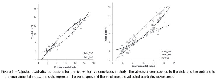
Although all the adjusted R2 are high and very similar, we have decided to use quadratic regression to express the responses of genotypes because this model is that for all genotypes it gives the best fit of the data, as can be seen from Table 4. The adjusted regression coefficients of the quadratic model, R2 and p-values arepresented in Table 5. Figure 1 represents the adjusted quadratic regressions for the five winter rye genotypes in study.
After rejecting the hypothesis that the regression is not a quadratic curve for each of the genotypes (p < 0.001, Table 5) we are led to test whether the regression curves are parallel for all five genotypes (cf. Table 1). The hypothesis that the regression lines are parallel is rejected (Table 6), as expected after analyzing Figure 1 and from a preliminary analysis where GEI was found in this data.
In the next step of investigating GEI we tried to find subgroups of genotypes where responses are parallel (or coincident). By simple inspection of the coefficients (Table 5), we can consider two groups of genotypes: (1) CHD_296; RAH_797 and URSUS; (2) RAH_596 and RAH_697. In this case this is in accordance with the preliminary analysis presented in Figure 1.
To quantify the differences we can use multiple comparison methods such as Scheffé (Scheffé, 1959; Miller, 1991). When using the Scheffé method, representing by f1-a, r, g the 1 - a quantile of the central F distribution with r and g degrees of freedom, and  , i = 1,...,I, m = 0,12 the variance of the regression coefficient bim, the pairs of quadratic regression coefficients which satisfy the condition ,
  m = 0, 1, 2, are different at the significance level α.
Since the regression coefficients b1 and b2 do not differ among environments (p < 0.05), we present in Table 7 only the results for the Scheffé multiple comparison method of the b0 coefficients.
The groups obtained with the Scheffé method at significance level 1 % are the same as those given by the simple inspection of the coefficients or by analysis of Figure 1.
The multiple comparison method of Scheffé made it possible to divide the genotypes into two groups: one group with upward-facing concavity (i.e. potential yield growth) and other with downward-facing concavity (i.e. the yield approaches saturation). Inspecting the coefficients, especially b2, it is possible to see the form of the yield curves. If b2 is positive, the curve will be convex, otherwise concave.
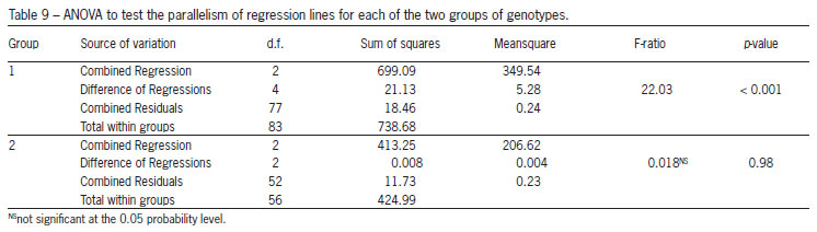
Table 8 shows the common regression coefficients for all genotypes together and each of the two groups obtained using the Scheffé multiple comparison method, while Table 9 gives the ANOVA to test the parallelism of regression lines for each of the two groups of genotypes. The hypotheses of parallelism between the quadratic regressions were rejected for the first group of genotypes (Table 9). However, we do not reject the same hypothesis for the second group. Hence, in this case, we can go one step further and test whether the regressions in the second group are coincident (hypothesis H01). From the ANOVA presented in Table 10 we reject that hypothesis, i.e. although the quadratic regression lines are parallel they are distinct. Therefore the adjusted regression functions for the genotypes RAH_596 and RAH_697 can be written as:
 RAH_596 = 6.229 - 0.397X + 0.066X2;
RAH_697 = 6.717- 0.397X + 0.066X2,
where the b1 and b2 are the common regression coefficients from Table 8 and the b0 coefficients are calculated according to expression (6).
We point out that we did not find groups of genotypes with identical regressions; this may be due to the high level of GEI. All that we can say is that genotypes RAH_596 and RAH_697 have yields parallel, with that of the second genotype a little higher.
Conclusions
The hypothesis of parallelism of regression curves was rejected, which is natural in multi-environment trials with interaction between genotype and environment. The main difference in the two subgroups of genotypes where the responses are parallel is that one group had upward-facing concavity (i.e. potential yield growth) and the other had downward-facing concavity (i.e. the yield approaches saturation), which can help breeders in their genotype selection. The approach proposed in this paper is general and applicable to any series of experiments conducted in multi-environment trials or simply to the case of two-way classified data.
Acknowledgments
Dulce G. Pereira is a member of the CIMA-UE, a research center financed by the Science and Technology Foundation, Portugal. The work was partially supported by Ministry of Science and Higher Education Grant N N310 447838, and by the Fundação para a Ciência e a Tecnologia (Portuguese Foundation for Science and Technology) through PEst-OE/MAT/UI0297/2011 (CMA). We thank the anonymous referees and the Associated Editor for their suggestions, which greatly improved the paper.
Received June 30, 2011
Accepted May 04, 2012
Edited by: Thomas Kumke
- Aastveit, A.H.; Mejza, S. 1992. A selected bibliography on statistical methods for the analysis of genotype x environment interaction. Biuletyn Oceny Odmian 25:83-97.
- Annicchiarico, P. 2002. Genotype x Environment Interactions: Challenges and Opportunities for Plant Breeding and Cultivar Recommendations. Food and Agricultural Organization, Rome, Italy. (FAO Plant Production and Protection Paper, 174).
- Digby, P.G.N. 1979. Modified joint regression-analysis for incomplete variety x environment data. Journal of Agricultural Science 93:81-86.
- Finlay, K.W.; Wilkinson, G.N. 1963. Analysis of adaptation in a plant-breeding programme. Australian Journal of Agricultural Research 14:742-754.
- Gabriel, K.R.; Zamir, S. 1979. Lower rank approximation of matrices by least-squares with any choice of weights. Technometrics 21:489-498.
- Gauch, H.G. 1992. Statistical Analysis of Regional Yield Trials: AMMI Analysis of Factorial Designs. Elsevier, Amsterdam, Netherlands.
- Gusmão, L. 1985. An adequate design for regression analysis of yield trials. Theoretical and Applied Genetics 71:314-319.
- Gusmão, L. 1986. Inadequacy of blocking in cultivar yield trials. Theoretical and Applied Genetics 72:98-104.
- Kang, M.S.; Gauch, H.G., eds. 1996. Genotype-by-environment interaction. CRC Press, Boca Ratón, FL, USA.
- Kleinbaum, D.G.; Kupper, L.L.; Nizam, A.; Muller, K.E. 2008. Applied Regression Analysis and Other Multivariable Methods. 4ed. Thompson Higher Education, Belmont, CA, USA.
- Mexia, J.T.; Pereira, D.G.; Baeta, J. 1999. L2 environmental indexes. Biometrical Letters 36:137-143.
- Miller, R.G. 1991. Simultaneous Statistical Inference. Springer, New York, NY, USA.
- Ng, M.P.; Williams, E.R. 2001. Joint-regression analysis for incomplete two-way tables. Australian & New Zealand Journal of Statistics 43:201-206.
- Pereira, D.G.; Mexia, J.T. 2010. Comparing double minimization and zig-zag algorithms in joint regression analysis: the complete case. Journal of Statistical Computation and Simulation 80:133-141.
- Pereira, D.G.; Rodrigues, P.C.; Mejza, S.; Mexia, J.T. 2011. A comparison between joint regression analysis and AMMI: a case study with barley. Journal of Statistical Computation and Simulation 82:193-207.
- Rodrigues, P.C.; Pereira, D.; Mexia, J.T. 2011. A comparison between JRA and AMMI: the robustness with increasing amounts of missing data. Scientia Agricola 68:679-686.
- Romagosa, I.; van Eeuwijk, F.A.; Thomas, W.T.B. 2009. Statistical analyses of genotype by environment data. v.3. In: Phohens, J.; Nuez, F.; Carena, M.J. eds. Handbook of Plant Breeding. Elsevier, New York, NY, USA.
- Scheffé, H. 1959. The Analysis of Variance. Wiley, New York, NY, USA.
- Williams, E.J. 1967. Regression Analysis. Wiley, New York, NY, USA.
Publication Dates
-
Publication in this collection
14 Nov 2012 -
Date of issue
Dec 2012
History
-
Received
30 June 2011 -
Accepted
04 May 2012