Applying the NDVI from satellite images in delimiting management zones for annual crops

ABSTRACT:

The utilization of Normalized Difference Vegetation Index (NDVI) data obtained through satellite images can technically improve the process of delimiting management zones (MZ) for annual crops, resulting in socio-economic and environmental benefits. The aim of this study was to compare delimited MZ, using crop productivity data, with delimited MZ using the NDVI obtained from satellite images in areas under a no-tillage system. The study was carried out in three areas located in the state of Rio Grande do Sul, Brazil. Three crop productivity maps, from 2009 to 2015, were used for each area, whereby the NDVI was calculated for each crop productivity map using images from the Landsat series of satellites. Descriptive and geostatistical analysis were conducted to determine the productivity and NDVI data. The MZ were then delimited using the fuzzy c-means algorithm. Spearman's correlation matrix was used to compare the methodologies used for delimiting the MZ. The MZ based on NDVI calculated from the satellite images correlated with the MZ based on crop productivity data (0.48 < r < 0.61), suggesting that the NDVI can replace or be complementary to productivity data in delimiting MZ for annual cropping systems.

Keywords:
fuzzy c-means clustering; productivity data; aerial images; vegetation index

Introduction

Increasing the productivity of an agricultural system, coupled with attractive economic return and minimal environment impacts, is one of the main challenges of the 21^st century (Godfray et al., 2010). Under this scenario, it is imperative that decision makers (e.g., farmers, consultants, extension agents) have access to specific information about the soil, cropping system and climate that directly and indirectly support the adoption of better management practice choices in each agricultural production system (Lee and Ehsani, 2015; Srbinovska et al., 2015).

The use of management zones (MZ) is an important approach that, among other benefits, it enables reductions in the production cost, while reducing the environmental impacts of agricultural activities (Kaffka et al., 2005; Moral et al., 2011). For farmers to be able to use MZ, the first step is to delimit those zones based on parameters that are generated which take into account different soil attributes (Santi et al., 2016; Damian et al., 2016), topographical components (Fraisse et al., 2001; Fridgen et al., 2004), vegetation indexes (Zhang et al., 2010; Chang et al., 2014), and the intrinsic parameters of each crop (El Nahry et al., 2011; Tagarakis et al., 2013). Among many options, crop productivity data has been considered the most important parameter for efficiently defining MZ in annual cropping systems (Buttafuoco et al., 2010; Betzek et al., 2018).

Crop productivity maps are created from the yield data collected by a set of sensors coupled to the harvesters together with positioning information systems (Blackmore and Moore, 1999). However, from the harvesting operation to elaboration of the productivity maps, errors attributed to the sensors, data logger, operating conditions, positioning or operator, can compromise the quality of the mapping (Arslan and Colvin, 2002). An interest in using vegetation indices as an alternative to productivity maps has emerged in recent years. Globally, the NDVI, calculated from satellite images (Tarnavsky et al., 2008) has been widely used, since it is closely correlated with crop productivity (Boken and Shaykewich, 2002; Sultana et al., 2014; Lopresti et al., 2015; Peralta et al., 2016). In addition, high resolution satellite images can be acquired at a low price, which allows for mapping large areas with low investments.

Understanding the relationship between MZ generated from productivity maps and those generated from NDVI obtained from satellite images is essential to increasing the efficiency of delimiting management zones. In this respect, the aim of this study was to evaluate the effectiveness of using NDVI obtained from satellite images compared to crop productivity maps to characterise management zones in areas under a no-tillage system in southern Brazil.

Materials and Methods

Study sites

The study was carried out in three areas in northern Rio Grande do Sul (RS) state, Brazil (Figure 1). Area 1 (27°42'38” S − 53°20'04” W; 559 m a.s.l) covering 117 ha and Area 2 (28°08'20” S − 53°31'07” W; 491 m a.s.l) covering 97 ha are located near Boa Vista das Missões city, whereas Area 3 (27°44'07“ S − 53°21'03“ W; 602 m a.s.l) covering 75 ha is located near Condor city. The climate in the region is humid subtropical with hot summers, type Cfa, with average maximum temperatures ≥ 22 °C, average minimum temperatures from −3 to 18 °C, and average annual precipitation between 1,900 and 2,200 mm (Alvares et al., 2013).

Figure 1
Geographical location of the experimental areas used in the study.

The regional landscape is characterized by gently rolling terrain, with the soil classified as a clayey Typic Hapludox (Soil Survey Staff, 2014) in the study areas. The management system used in the selected areas included the adoption of a no-tillage system (NTS) for more than 20 years, and the use of precision agriculture tools in the last 10 years, such as georeferenced soil sampling, soil mapping, variable rate application of lime and fertilisers, and crop yield mapping.

Productivity maps

The crop productivity data were collected by a yield monitor for grain yield and moisture mapping of harvested grains. The system consisted of an impact-plate instant grain sensor installed at the end of the clean grain elevator. In addition, the harvester had a speed monitoring system coupled with information on platform width, and stored the yield information based on georeferenced GPS signals.

The gross productivity databases were filtered to eliminate outliers as described by Menegatti and Molin (2003). The elimination criterion for the outliers included points that had a coefficient of variation (CV) greater than 30 %, which characterize inconsistent productivity (Suszek et al., 2011). For this study, three productivity maps with complete dataset were used for each area: i) Area 1: White Oats (2010), Wheat (2013), and Soybean (2014-2015); ii) Area 2: Wheat (2009), Wheat (2014) and Soybean (2014-2015); and iii) Area 3: Maize (2009-2010), Wheat (2010) and Soybean (2011-2012).

Satellite images

The images from the Landsat series of satellites (Landsat 7 and 8) were obtained from USGS Earth Explorer, a free access database. The images were downloaded in GeoTiff format (Level 1), presenting pixel sizes of 30 m. Atmospheric correction was performed using the semi-automatic classification plugin in QGIS 2.18 (Congedo, 2016) in order to obtain surface reflectance without the interference of atmospheric gases. Landsat 7 images were used for crop seasons from 2009 to 2012, and Landsat 8 images for crop seasons from 2013 to 2015.

One satellite image was selected for each area and crop under study with a date that represented the crop cycle, as described in Table 1. Satellite images were chosen that displayed the best quality, i.e. with no cloud cover in the area of study. The NDVI was calculated from the satellite images using the QuantumGIS (OSGeo) software according to Equation 1:

(1) $$NDVI=\frac{\left(NIR-R\right)}{(NIR+R}$$

Table 1
Dates for the sowing and harvesting of crops, and the acquisition of satellite imagery, used in calculating the NDVI for annual crops in southern Brazil.

Site	Crop	Crop cycle		Acquisition of satellite images
		Sowing	Harvest	Date	Phenological stage
Area 1	White Oats	05/26/2010	10/19/2010	08/20/2010	60 (end of earing)1
	Wheat	06/17/2013	11/01/2013	09/13/2013	55 (50 % earing)1
	Soybean	11/08/2014	03/25/2015	01/22/2015	R 5.3 (pods with 26 % and 50 % seeding)2
Area 2	Wheat	06/13/2009	10/28/2009	08/17/2009	52 (20 % earing)1
	Wheat	06/05/2014	10/21/2014	09/08/2014	50 (first ear visible)1
	Soybean	11/10/2014	03/28/2015	01/14/2015	R 4 (completely developed pods)2
Area 3	Maize	10/20/2009	03/09/2010	01/24/2010	R 4 (pasty grain)3
	Wheat	06/10/2010	10/30/2010	08/20/2010	52 (20 % earing)1
	Soybean	11/15/2011	03/25/2012	01/06/2012	R 5.1 (10 % seeding)2

• ¹
  Zadoks et al. (1974);
• ²
  Ritchie et al. (1982);
• ³
  Ritchie et al. (1993).

where: NDVI is the Normalised Difference Vegetation Index (unitless); NIR the near-infrared region; R the red region. In Landsat 7 the NIR corresponds to band 4 (spectral resolution of 0.76 − 0.90 μm) and the R to band 3 (spectral resolution of 0.63 − 0.69 μm). In Landsat 8 the NIR corresponds to band 5 (spectral resolution of 0.85 − 0.89 μm) and the R to band 4 (spectral resolution of 0.63 − 0.68 μm).

To avoid errors due to the overlapping of satellite images in the study area, especially considering the edges of the area that were close to trees, water reservoirs, or bare soil among others, the NDVI data was filtered for each situation under evaluation by excluding NDVI values in a 10 m strip around the perimeter of the area.

After calculating the NDVI, for each pixel a centroid was added corresponding to the NDVI value at the centre of the pixel, with the centroids inheriting the same attributes as the polygons generated from the pixels. This procedure was used to standardise the NDVI and productivity data, allowing for a comparison between these parameters.

Data analysis

A regular 30 × 30 m mesh (0.09 ha) was overlapped on the productivity and NDVI maps. This procedure standardised the same number of points (cells) for each map, allowing for a temporal comparison of the maps. The size of the grid was defined by the pixel size of the satellite image (30 m).

Exploratory analysis (descriptive statistic) was conducted to verify data distribution using the SAS software (Statistical Analysis System, version 9.3). The statistical parameters determined were: minimum, mean, maximum, standard deviation and the coefficients of variation (CV %), asymmetry (Cs) and kurtosis (Ck). Based on the values for CV (%), data dispersion was classified as low for a CV < 15 %; moderate for a CV of 15 to 35 %; and high for a CV > 35 % (Wilding and Drees, 1983). The existence of a central tendency (normality) in the original data was verified by means of the W-test (p > 0.05).

Considering that the majority of the productivity and NDVI data did not follow a normal distribution of frequency, Spearman's nonparametric correlation matrix was used to evaluate the spatio-temporal correlation between these two variables. Only the productivity and NDVI data for crops with a Spearman correlation coefficients greater than 0.30 were included in the study, in order to reduce the uncertainties related to the delimitation of the management zones. The amount of data which did not meet this criterion ranged from 8 to 12 % in the three study areas.

Geostatistical analysis of the productivity and NDVI data was carried out using semivariograms, with adjustments made by means of theoretical models (spherical, exponential, Gaussian and linear) using the GS+ Gamma Design Software (Robertson, 1998). The fit of the models was based on the best coefficient of determination (r²) and the lowest residual sum of squares (RSS) obtained by the cross-validation technique. The following parameters were defined for each model: theoretical, nugget effect (C₀), contribution (C₁), sill (C₀ + C₁) and range (r). From the parameters obtained in fitting the semivariogram model, thematic maps were generated using kriging as the interpolator.

Management zones

Delimitation of the management zones was determined through fuzzy c-means clustering algorithms, to partition spatial observations into clusters. The analysis was done using the Management Zone Analyst (MZA) 1.0.1 software (Fridgen et al., 2004).

The fuzziness performance index (FPI) and normalised classification entropy index (NCE) were used to determine the best number of clusters (management zones) as well as their overall performance. The FPI (Equation 2) is a measure of the degree of different association classes (imprecision), where the values range from 0 to 1 (Odeh et al., 1992). The NCE (Equation 3) is used to decide how many clusters are suitable for defining the management zones (Bezdek, 1981). The ideal number of clusters occurs when the two indices are at their minimum (Fridgen et al., 2004).

(2) $$FPI=1-\frac{c}{\left(c-1\right)}\left[1-\frac{1}{n}{\displaystyle \sum _{k=1}^n{\displaystyle \sum _{i=1}^c{\left(u_{ik}\right)}^2}}\right]$$

(3) $$NCE=\frac{n}{\left(n-c\right)}\left[-\frac{1}{n}{\displaystyle \sum _{k=1}^n{\displaystyle \sum _{i=1}^c{u}_{ik}}{\log }_a}\left(u_{ik}\right)\right]$$

where: c = values of the centroids in the cluster; u_ik, the values for each observation K in cluster i; log_a, any positive integer; and n, the number of data analysed.

The configurations chosen were a measure of Euclidean similarity: fuzzy exponent = 1.3, maximum number of iterations = 300, convergence criterion = 0.0001, minimum number of zones = 2, and the maximum number of zones = 8.

The accuracy of mapping of management zones delimited with productivity data and NDVI was performed using the Kappa coefficient. In addition, data from seven replicates were randomly collected in each zone, where each replicate was composed of 20 sampling points of NDVI, and were subjected to an analysis of variance (ANOVA). When ANOVA was significant (F-test, p < 0.05), the mean values were compared according to Tukey's test (p ≤ 0.05).

Results and Discussion

Exploratory data analysis

Descriptive statistical analysis revealed that for most crops the productivity and NDVI data did not follow a normal distribution of frequency (Table 2). This lack of normality may be associated with the high number of observations, which made it possible to detect the spatial variability of the productivity and NDVI data with a high degree of resolution.

Table 2
Descriptive statistics of the productivity and NDVI data for different annual crops in southern Brazil.

Site	Crop season	Minimum	Mean	Maximum	CV %1	SD2	Cs3	Ck4	W5
Area 1	Crop productivity (kg ha –1)
	White Oats/2010	710.90	2435.94	3637.01	20.51	499.71	-0.33	-0.34	0.98*
	Wheat/2013	2818.13	3850.33	5109.63	9.07	349.40	0.05	0.12	0.74ns
	Soybean/2014	2409.28	3778.93	4535.14	8.27	309.78	-1..27	2.17	0.91*
	NDVI
	White Oats /2010	0.25	0.47	0.51	7.37	0.04	-4.05	35.96	0.74*
	Wheat/2013	0.29	0.55	0.63	7.19	0.03	-3.99	25.52	0.66*
	Soybean/2014	0.31	0.51	0.66	8.70	0.04	-5.87	54.31	0.57*
Area 2	Crop productivity (kg ha –1)
	Wheat/2009	407.17	3797.76	7483.28	18.17	690.14	-0.27	3.66	0.96*
	Wheat/2014	502.13	2400.03	7861.55	29.22	701.24	2.78	16.16	0.78*
	Soybean/2014	1467.56	3422.64	4769.56	15.39	526.76	-0.56	-0.10	0.97*
	NDVI
	Wheat//2009	0.24	0.35	0.66	2.30	0.02	0.17	0.01	0.99*
	Wheat/2014	0.65	0.82	0.87	4.03	0.03	-1.91	3.79	0.78*
	Soybean/2014	0.27	0.43	0.56	9.97	0.04	-0.26	0.52	0.99
Area 3	Crop productivity (kg ha –1)
	Maize/2009	1338.00	7538.90	13455.10	22.32	1682.75	-0.18	1.08	0.98*
	Wheat/2010	755.80	3040.43	4465.80	13.32	404.62	-0.81	2.58	0.96
	Soybean/2011	1152.83	4080.89	5013.35	9.98	399.70	-2.14	8.92	0.85
	NDVI
	Maize/2009	0.56	0.77	0.83	5.44	0.04	-1.35	2.03	0.89*
	Wheat/2010	0.47	0.64	0.69	4.90	0.03	-1.72	4.41	0.87*
	Soybean/2011	0.22	0.58	0.84	12.02	0.07	-1.72	8.56	0.84*

• ¹
  Coefficient of variation;
• ²
  Standard deviation;
• ³
  Coefficient of asymmetry;
• ⁴
  Coefficient of kurtosis;
• ⁵
  Shapiro-Wilk test for normal distribution, where:
• ^*
  Significant at a level of < 0.05 and
• ^ns
  not significant. When significant, this indicates that the hypothesis for normal distribution is rejected.

The productivity data had CV values ranging from 8 to 29 % (Table 2). In areas 1, 2 and 3, the greatest variation in the data was observed for White Oats/2010, Wheat/2014 and Maize/2009 respectively, with CVs classified as moderate (Wilding and Drees, 1983). Thus, our results indicated that there is no universal pattern of variation per crop, confirming that productivity data of different crops need to be included in delimiting MZ so as to cover the spatio-temporal variation of productivity within diversified cropping systems.

The NDVI data showed lower CV values (i.e., ranging from 2 to 12 %) than those verified for productivity. These results are consistent with those obtained in other studies (Zerbato et al., 2016; Barbanti et al., 2017), and may be due to the fact that NVDI values range from 0 to 1. Another factor that contributes to lower variation of NDVI data is associated with the phenological stages of crops at the moment of the image acquisitions. In this study, the images were obtained when the crops presented a high leaf area index (after crops had reached maximum vegetative growth), which resulted in lower interferences affecting NDVI values.

Contrasting results were found for NDVI values and productivity values for soybean and wheat crops in the same area, as well as in different areas (Table 2). The NDVI values for wheat did not follow the magnitude of the variation in productivity, suggesting that this crop presents high sensitivity to edaphoclimatic variations during its cycle (Roman et al., 2008). However, the soybean crop showed higher stability of NDVI values in relation to productivity values in the three study areas, likely associated with the high plasticity of this crop (Ferreira et al., 2018), which enables adaptation to different environmental and management conditions (e.g., altitude, latitude, soil texture, soil fertility, sowing date, plant population and line spacing).

Spearman's correlation

In general, the productivity and the NDVI data showed significant correlation (Table 3). In Area 1, the correlation coefficients were considered high compared to the other areas, of 0.56, 0.61 and 0.56 for the productivity data for White Oats/2010, Wheat/2013, and Soybean/2014, and their respective NDVI data. In contrast, the lowest values for the correlation coefficients were found in Area 2, despite their being considered acceptable according to the previously adopted criterion (> 0.30), being 0.48, 0.31 and 0.47 fo the data for Wheat/2009, Wheat/2014 and Soybean/2014, and their NDVI data. In Area 3, the correlation coefficients were close to those found for Area 1, of 0.51, 0.58 and 0.49 for the productivity data for Wheat/2009, Wheat/2014 and Soybean/2014, and their respective NDVI data.

Table 3
Spearman's correlation matrix (p ≤ 0.01) between productivity and NDVI data for different annual crops in southern Brazil.

Area 1
	Pwo10	Pw13	Ps14	Nwo10	Nw13	Ns14
Pwo10	-
Pw13	0.03	-
Ps14	0.32	0.27	-
Nwo10	0.56	0.24	0.27	-
Nw13	0.03	0.61	0.19	0.27	-
Ns14	0.20	0.06	0.56	0.26	0.48	-
Area 2
	Pw09	Pw14	Ps14	Nw09	Nw14	Ns14
Pw09	-
Pw14	0.23	-
Ps14	0.36	0.18	-
Nw09	0.48	0.03	0.05	-
Nw14	0.29	0.31	0.32	0.02	-
Ns14	0.08	0.10	0.47	0.06	0.10	-
Area 3
	Pm09	Pw10	Ps11	Nm09	Nw10	Ns11
Pm09	-
Pw10	0.32	-
Ps11	0.10	0.25	-
Nm09	0.51	0.04	0.15	-
Nw10	0.04	0.58	0.22	0.21	-
Ns11	0.15	0.10	0.49	0.37	0.11	-

• Values highlighted in bold show a correlation > 0.30. Area 1 = Productivity data for White Oats/2010 (Pwo10); Productivity data for Wheat/2013 (Pw13); Productivity data for Soybean/2014 (Ps14); NDVI for White Oats/2010 (Nwo10); NDVI for Wheat/2013 (Nw13); NDVI for Soybean/2014 (Ns14). Area 2 = Productivity data for Wheat/2009 (Pw09); Productivity data for Wheat/2014 (Pw14); Productivity data for Soybean/2014 (Ps14); NDVI for Wheat/2009 (Nw09); NDVI for Wheat/2014 (Nw14); NDVI for Soybean/2014 (Ns14). Area 3 = Productivity data for Maize/2009 (Pm09); Productivity data for Wheat/2010 (Pw10); productivity data for Soybean/2011 (Ps11); NDVI for Maize/2009 (Nm09); NDVI for Wheat/2010 (Nw10); NDVI for Soybean/2011 (Ns11).

The significant correlations found between the productivity and the NDVI data confirmed that the NDVI calculated from satellite images can be used as a parameter to delimiting management zones for annual cropping systems. These results agree with those previously reported by Zhang et al. (2010), who also found correlation between productivity and the NDVI calculated from satellite images, indicating the strong relationship between the spectral reflectance of the crops which can be used to map their productivity.

Geostatistical analysis

The results of the geostatistical analysis indicated that productivity and NDVI data, obtained for each crop in the three areas, are spatially dependent (Table 4), allowing for interpolation and spatialisation of the data in maps (Vieira, 2000), which are useful tools to guide management interventions.

Table 4
Geostatistical analysis of the crop productivity and NDVI data for annual crops in southern Brazil.

	Crop season	Nugget Effect (C0)	Sill (C0+C1)	Contribution (C1)	Range (a)	Model	r2
Area 1	Crop productivity (kg ha –1)
	White Oats/2010	46800	163199	116399	732	Exponencial	0.79
	Wheat/2013	355000	1474000	1119000	584	Esférico	0.88
	Soybean/2014	337000	1016000	679000	665	Esférico	0.95
	NDVI
	White Oats/2010	0.00036	0.00162	0.00126	995	Gaussiano	0.88
	Wheat/2013	0.00062	0.00209	0.00147	797	Exponencial	0.73
	Soybean/2014	0.00077	0.00171	0.00094	826	Exponencial	0.95
Area 2	Crop productivity (kg ha –1)
	Wheat//2009	297640	612622	314982	779	Esférico	0.89
	Wheat/2014	319000	698100	379100	832	Esférico	0.82
	Soybean/2014	103900	300000	196100	492	Exponencial	0.88
	NDVI
	Wheat//2009	0.00001	0.00407	0.00406	851	Exponencial	0.78
	Wheat/2014	0.00126	0.00663	0.00537	979	Exponencial	0.84
	Soybean/2014	0.00083	0.00864	0.00781	935	Exponencial	0.89
Area 3	Crop productivity (kg ha –1)
	Maize/2009	2303592	3024705	721113	852	Esférico	0.76
	Wheat/2010	111368	181228	69860	870	Esférico	0.81
	Soybean/2011	142393	180083	37690	789	Esférico	0.83
	NDVI
	Maize/2009	0.00081	0.00267	0.00186	902	Exponencial	0.80
	Wheat/2010	0.00085	0.00210	0.00125	954	Exponencial	0.85
	Soybean/2011	0.00109	0.00392	0.00283	886	Exponencial	0.75

The spatial variability of productivity data was predominantly adjusted to the spherical model, whereas the NDVI data were adjusted to the exponential model (Table 4). The spherical and exponential models have been widely used to evaluate the spatial variability of the productivity (Damian et al., 2017; Souza et al., 2016) and NDVI of different agricultural cropping systems (Ji et al., 2014; Ungaro et al., 2017).

Similar range values obtained from semivariograms were found in the three study areas, varying from 492 to 870 m for the productivity data, and from 797 to 995 m for the NDVI data. For both variables, the greatest ranges were observed in the Wheat crop, and the lowest values in the Soybean crop. This result can be attributed to the stronger spatial dependence of the productivity data compared to NDVI data, providing a wider range of values. All the models fit the acceptance criteria in relation to the parameters of the adjusted semivariograms, i.e. the r² of the semivariogram was equal to or greater than 0.70 and significant to 5 % in the cross validation.

Mapping the values for crop productivity and NDVI

From the mapping of crop productivity in Area 1, a band of high productivity can be seen in the central part of the map, extending from the south to the north, especially for White Oats/2010 (Figure 2A) and Soybean/2014 (Figure 2C). Despite a number of similarities, this pattern was not repeated on the map for Wheat/2013 (Figure 2B); however, it was possible to identify sites of contrasting productivity on the three productivity maps. In Area 2, a consistent productivity pattern was obtained for the three crops, with higher yields concentrated in the western region of the maps (Figure 2D-F). In Area 3, the maps of Maize/2009 (Figure 2G) and Wheat/2010 (Figure 2H) indicated greater productivity in the southern and central regions of the maps, while high yields were also found in the northern region for Soybean/2011 (Figure 2I).

Figure 2
Spatial distribution (kg ha^–1) of grain productivity in the crops of White Oats/2010 (A), Wheat/2013 (B) and Soybean/2014 (C) for Area 1, Wheat/2009 (D), Wheat/2014 (E) and Soybean/2014 (F) for Area 2, and Maize/2009 (G) Wheat/2010 (H) and Soybean/2011 (I) for Area 3.

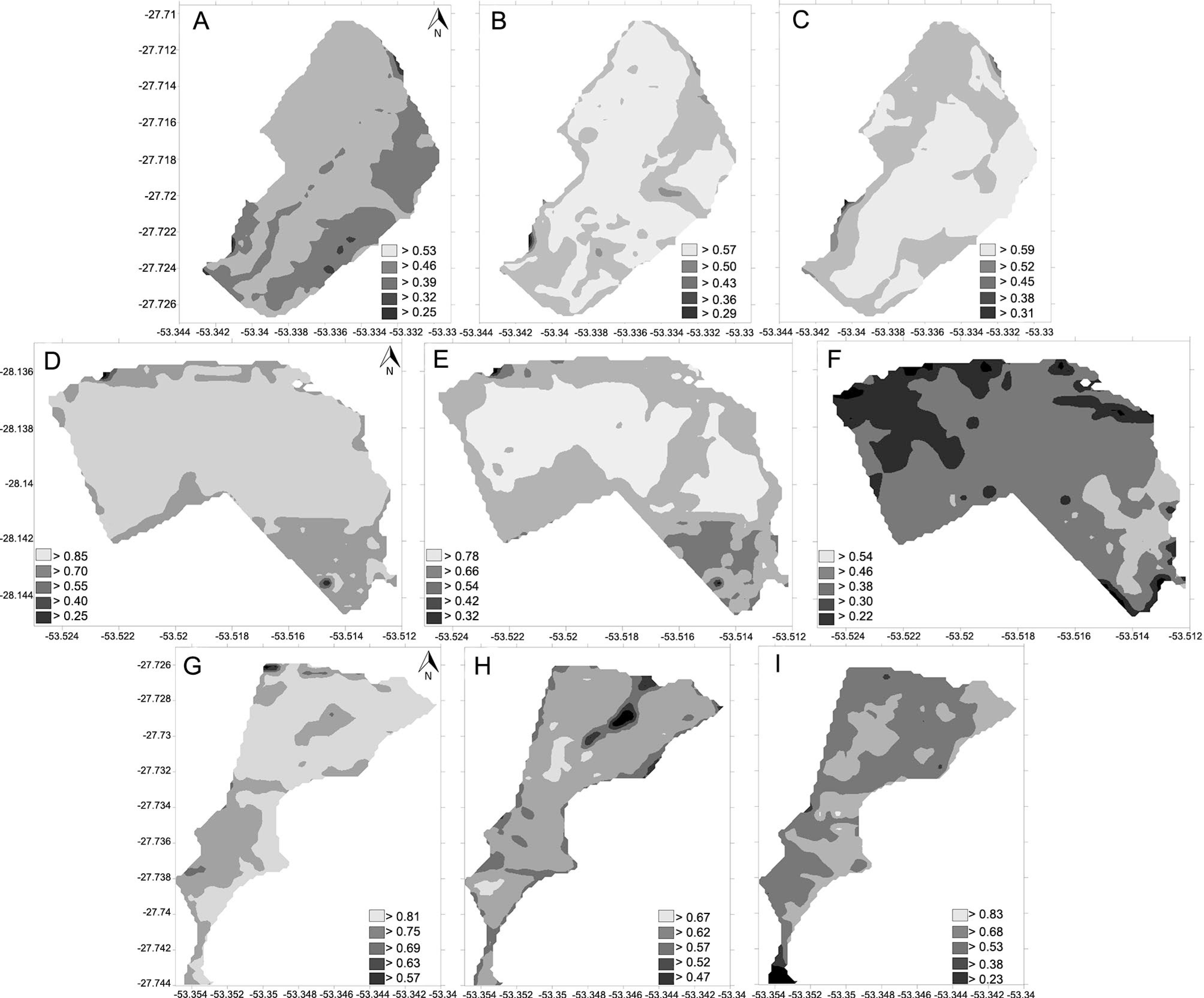
In general, the NDVI data converged with the maps of the productivity data, showing that regions of higher productivity also had higher NDVI values (Figure 3A-I). The efficiency of the NDVI obtained from satellite images and their agreement with productivity maps had also been reported in other studies (Groten, 1993; Boken and Shaykewich, 2002; Lopresti et al., 2015), indicating the close link between NDVI and crop productivity.

Figure 3
Spatial distribution of the NDVI for the crops of White Oats/2010 (A), Wheat/2013 (B) and Soybean/2014 (C) for Area 1, Wheat/2009 (D), Wheat/2014 (E) and Soybean/2014 (F) for Area 2, and Maize/2009 (G) Wheat/2010 (H) and Soybean/2011 (I) for Area 3.

Delimitation of the management zones

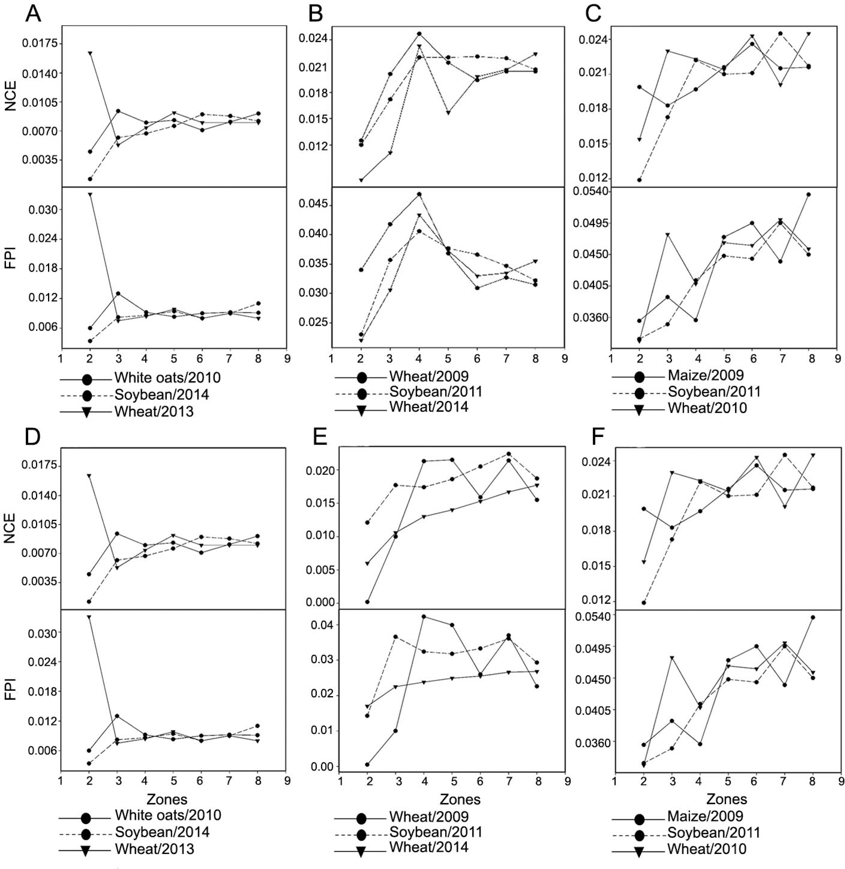
The results for the fuzziness performance index (FPI) and normalised classification entropy index (NCE) showed similar responses between both the productivity data and the NDVI data. These indexes allowing for a consistent analysis of the differentiation between the management zones, from the eight management zones under test. Fridgen et al. (2004) emphasize that in certain cases, the response of the variables studied within each index can be strikingly different, and it is not possible to identify the number of convergent zone. In cases of extreme discrepancy, the final decision of how many classes to use depends on additional analysis, such as comparing defined management zones with different input variables to determine which are the most important (Alves et al., 2013), or defining the possible number of representative classes for the remaining variables.

According to Fridgen et al. (2004), the lowest values of the NCE and FPI indices result in a suitable number of management zones, since it shows the least membership sharing (FPI) or the greatest amount of organisation (NCE) in the clustering process. Based on this criterion, and for the two indices under test, the results showed that out of the eight management zones tested, two zones would be ideal for representing the set of three productivity maps (Figure 4A-F). In addition, no significant improvement was seen in the FPI and NCE indices when the number of classes was greater than two, suggesting that with the increase in index values there was an increase in the number of clusters, with a consequent increase in data variability.

Figure 4
Fuzziness performance index (FPI) and normalised classification entropy index (NCE) for the productivity data in Areas 1 (A), 2 (B) and 3 (C), and for the NDVI data in Areas 1 (D), 2 (E) and 3 (F).

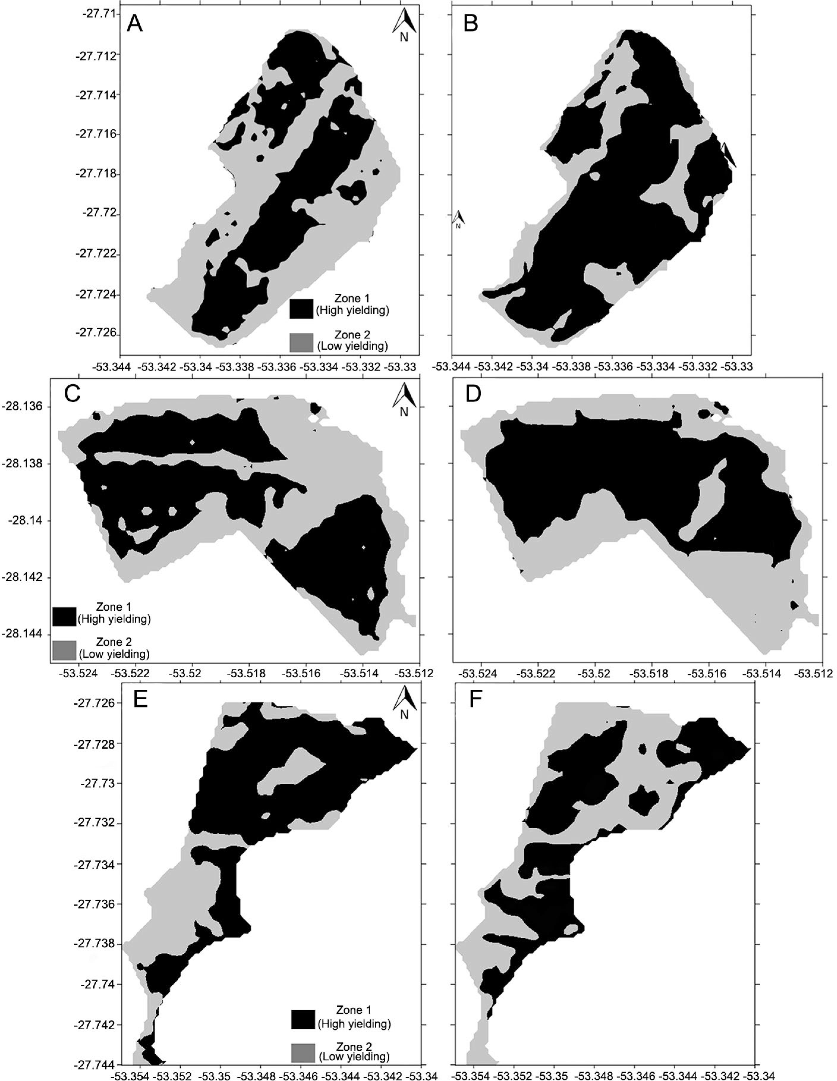
After defining the ideal number of management zones for each area, both the productivity maps and the NDVI maps were grouped by the fuzzy c-means algorithm, generating new maps that show only the two zones (Figure 5A-F), where Zone 1 is a zone of high potential and Zone 2 a zone of low potential, so called by Damian et al. (2016). As can be seen, the management zones delimited using the NDVI showed high similarity with the delimited management zone using the productivity data for the three areas.

Figure 5
Maps of the management zones, created based on the clustering of productivity and NDVI data for Areas 1 (A and B), 2 (C and D) and 3 (E and F) respectively.

The percentage of the area within each MZ was similar, regardless of study site (Table 5). The variation between the delimited MZ with the productivity data and NDVI were 7 to 10 % for areas 1 and 2 and 19 to 20 % for area 3. Kappa coefficient values were classified as “good” (0.48) and “excellent” (0.81), according to the classification proposed by Landis and Koch (1977), showing that the delimited management zone maps with productivity data and NDVI present great similarity.

Table 5
Classification qualitative attributes of the two management zones (Zone 1 - high yielding potential; Zone 2 - low yielding potential) delimited with crop productivity and NDVI data.

		Zone 1		Zone 2
		Percent of area	Kappa coefficient	Percent of area	Kappa coefficient
		%		%
Area 1	Crop productivity	46.32	0.81	53.68	0.78
	NDVI	53.67		46.32
Area 2	Crop productivity	44.93	0.73	55.07	0.71
	NDVI	54.53		45.47
Area 3	Crop productivity	59.62	0.56	39.38	0.48
	NDVI	40.25		59.79

In addition to creating similar maps, the fuzzy c-means algorithm was highly efficient in delimiting management zones of contrasting productive potential (Table 6). In general, irrespective of the parameter used to delimit the management zones (productivity or NDVI data), the values measured for productivity and NDVI were significantly different between Zones 1 and 2. Only in the case of Wheat/2014 in Area 2 was the difference not significant, despite the values showing this same pattern for the other crops and areas.

Table 6
Comparison of the mean crop productivity and the NDVI values for different crops in two management zones (Zone 1 - high yielding potential; Zone 2 - low yielding potential).

		Crop productivity /Management zones
		White oats/2010	Wheat/2013	Soybean/2014	NDVI-White oats/2010	NDVI-Wheat/2013	NDVI-Soybean/2014
Area 1	Zone 1	4020.12 a*	4297.35 a	3986.21 a	0.42 a	0.48 a	0.44 a
	Zone 2	3116.35 b	3252.32 b	3696.14 b	0.36 b	0.37 b	0.39 b
	NDVI/Management zones
	Zone 1	4086.15 a	4187.32 a	3956.22 a	0.43 a	0.47 a	0.52 a
	Zone 2	3199.19 b	3102.02 b	3596.23 b	0.34 b	0.40 b	0.44 b
	Crop productivity/Management zones
Area 2		Wheat/2009	Wheat/2014	Soybean/2014	NDVI-Wheat/2009	NDVI-Wheat/2014	NDVI-Soybean/2014
	Zone 1	4517.25 a	2242.40 a	4105.80 a	0.47 a	0.80 a	0.48 a
	Zone 2	3481.42 b	2093.23 a	2599.50 b	0.25 b	0.79 a	0.33 b
	NDVI/Management zones
	Zone 1	4514.52 a	1985.27 a	4089.56 a	0.45 a	0.75 a	0.50 a
	Zone 2	3481.36 b	1714.63 a	2800.03 b	0.28 b	0.72 a	0.35 b
	Crop productivity/Management zones
		Maize/2009	Wheat/2010	Soybean/2011	NDVI- Maize/2009	NDVI-Wheat/2010	NDVI-Soybean/2011
Area 3	Zone 1	7500.36 a	3472 a	4745 a	0.79 a	0.63 a	0.64 a
	Zone 2	6515.32 b	2317 b	3844 b	0.70 b	0.60 b	0.86 b
	NDVI/Management zones
	Zone 1	8546 a	3489 a	4022 a	0.78 a	0.66 a	0.62 a
	Zone 2	5889 b	2919 b	3759 b	0.69 b	0.60 b	0.52 b

• ^*
  Mean values followed by the same letter do not differ statistically by Tukey's test at 5 % probability (p ≤ 0.05).

Our findings confirm that the NDVI obtained from satellite images, the factors that increase errors (e.g., image overlap, presence of clouds, and stage of crop cycle among others) when suitably considered, can replace or be used in a complementary way for productivity data for delimiting management zones for annual crops. It is worth highlighting that definition of management zones should be based on spatial information that is stable or predictable over time and that crop information, such as NDVI, is the best way to diagnose such variations in the field (Li et al., 2007).

Conclusions

The delimitation of management zones using NDVI data generated from satellite images showed high convergence with the delimited management zones using productivity data. Therefore, NDVI data can efficiently substitute or complement a series of productivity maps for delimiting management zones, especially when it is difficult or not possible to obtain productivity data through the systems coupled to harvesters.

The use of the NDVI from satellite images as a parameter to delimit management zones for annual cropping systems may represent an important advance in Brazilian agriculture, and may provide more efficient use of resources (i.e., seeds, fertilizers, water and pesticides), and positive feedback in terms of agronomy, socio-economics and the environment.

Acknowledgments

The authors would like to thank Fabiano Paganella (GeoAgro) for his significant support during this research.

References

• Alves, S.M.F.; Alcântara, G.R.; Reis, E.F.; Queiroz, D.M.; Valente, D.S.M. 2013. Definition of management zones from maps of electrical conductivity and organic matter. Bioscience Journal 29: 104-114 (in Portuguese, with abstract in English).
• Alvares, C.A.; Stape, J.L.; Sentelhas, P.C.; De Moraes, G.J.L.; Sparovek, G. 2013. Köppen's climate classification map for Brazil. Meteorologische Zeitschrift 22: 711-728.
• Arslan, S.; Colvin, T.S. 2002. Grain yield mapping: yield sensing, yield reconstruction, and errors. Precision Agriculture 3: 135-154.
• Barbanti, L.; Adroher, J.; Damian, J.M.; Di Virgilio, N.; Falsone, G.; Zucchelli, M.; Martelli, R. 2017. Assessing wheat spatial variation based on proximal and remote spectral vegetation indices and soil properties. Italian Journal of Agronomy 21: 1-31.
• Blackmore, S.; Moore, M. 1999. Remedial correction of yield map data. Precision Agriculture 1: 53-66.
• Bezdek, J.C. 1981. Pattern Recognition with Fuzzy Objective Function Algorithms. Kluwer, Ewing, NJ, USA.
• Betzek, N.M.; Souza, E.G.; Bazzi, C.L.; Schenatto, K.; Gavioli, A. 2018. Rectification methods for optimization of management zones. Computers and Electronics in Agriculture 146: 1-11.
• Boken, V.K.; Shaykewich, C.F. 2002. Improving an operational wheat yield model using phenological phase-based normalized difference vegetation index. International Journal of Remote Sensing 23: 4155-4168.
• Buttafuoco, G.; Castrignano, A.; Colecchia, A.S.; Ricca, N. 2010. Delineation of management zones using soil properties and a multivariate geostatistical approach. Italian Journal of Agronomy 5: 323-332.
• Chang, D.; Zhang, J.; Zhu, L.; Ge, S.H.; Li, P.Y.; Liu, G.S. 2014. Delineation of management zones using an active canopy sensor for a tobacco field. Computers and Electronics in Agriculture 109: 172-178.
• Congedo, L. 2016. Semi-automatic classification plugin - Usermanual. Technical Report. DOI: 10.13140/RG.2.2.29474.02242/1
  » https://doi.org/10.13140/RG.2.2.29474.02242/1
• Damian, J.M.; Pias, O.H.C.; Santi, A.L.; Virgilio, N.; Berghetti, J.; Barbanti, L.; Martelli, R. 2016. Delineating management zones for precision agriculture applications: a case study on wheat in sub-tropical Brazil. Italian Journal of Agronomy 11: 171-179.
• Damian, J.M.; Santi, A.L.; Fornari, M.; Da Ros, C.O.; Eschner, V.L. 2017. Monitoring variability in cash-crop yield caused by previous cultivation of a cover crop under a no-tillage system. Computers and Electronics in Agriculture 142: 607-621.
• El Nahry, A.H.; Ali, R.R.; El Baroudy, A.A. 2011. An approach for precision farming under pivot irrigation system using remote sensing and GIS techniques. Agricultural Water Management 98: 517-531.
• Fraisse, C.W.; Sudduth, K.A.; Kitchen, N.R. 2001. Delineation of site-specific management zones by unsupervised classification of topographic attributes and soil electrical conductivity. Transactions of the ASAE 44:155-166.
• Fridgen, J.J.; Kitchen, N.R.; Sudduth, K.A.; Drummond, S.T.; Wiebold, W.J.; Fraisse, C.W. 2004. Management zone analyst (MZA): Software for subfield management zone delineation. Agronomy Journal 96: 100-108.
• Ferreira, A.S.; Balbinot Junior, A.A.; Werner, F.; Franchini, J.C.; Zucareli, C. 2018. Soybean agronomic performance in response to seeding rate and phosphate and potassium fertilization. Revista Brasileira de Engenharia Agrícola e Ambiental 22: 151-157.
• Groten, S.M.E. 1993. NDVI-crop monitoring and early yield assessment of Burkina Faso. International Journal of Remote Sensing 14: 1495-1515.
• Godfray, H.C.; Beddington, J.R.; Crute, I.R.; Haddad, L.; Lawrence, D.; Pretty, J.; Robinson, S.; Thomas, S.M.; Toulmin, C. 2010. Food security: the challenge of feeding 9 billion people. Science 327: 812-818.
• Ji, L.; Zhang, L.; Rover, J.; Wyile, B.K.; Chen, X. 2014. Geostatistical estimation of signal-to-noise ratios for spectral vegetation indices. ISPRS Journal of Photogrammetry and Remote Sensing 96: 20-27.
• Kaffka, S.R.; Lesch, S.M.; Bali, K.M.; Corwin, D.L. 2005. Site-specific management in salt-affected sugar beet fields using electromagnetic induction. Computers and Electronics in Agriculture 46: 329-350.
• Landis, J.R.; Koch, G.G. 1977. The measurement of observer agreement for categorical data. Biometrics 33: 159-174.
• Lopresti, M.F.; Di Bella, C.M.; Degioanni, A.J. 2015. Relationship between MODIS-NDVI data and wheat yield: a case study in northern Buenos Aires province, Argentina. Information Processing in Agriculture 2: 73-84.
• Lee, W.; Ehsani, R. 2015. Sensing systems for precision agriculture in Florida. Computers and Electronics in Agriculture 112: 2-9.
• Li, Y.; Zhou, S.; Feng, L.; Houng Yi, L. 2007. Delineation of site-specific management zones using fuzzy clustering analysis in a coastal saline land. Computers and Electronics in Agriculture 56: 174-186.
• Menegatti, L.A.A.; Molin, J.P. 2003. Methodology for identification and characterization of errors in yield maps. Revista Brasileira de Engenharia Agrícola e Ambiental 7: 367-374 (in Portuguese, with abstract in English).
• Moral, F.J.; Terrón, J.M.; Rebollo, F.J. 2011. Site-specific management zones based on the Rasch model and geostatistical techniques. Computers and Electronics in Agriculture 75: 223-230.
• Odeh, I.O.A.; Chittleborough, D.J.; McBratney, A.B. 1992. Soil pattern recognition with fuzzy-c-means: application to classification and soil-landform interrelationships. Soil Science Society of America Journal 56: 505-516.
• Peralta, N.R.; Assefa, Y.; Du, J.; Barden, C.J.; Ciampitti, I.A. 2016. Mid-season high-resolution satellite imagery for forecasting site-specific corn yield. Remote Sensing 8: 1-16.
• Robertson, G.P. 1998. GS+: Geostatistics for the Environmental Sciences. Gamma Design Software, Plainwell, MI, USA.
• Roman, M.; Uribe-Opazo, M.A.; Nóbrega, L.H.P.; Johann, J.A. 2008. Spatial variability of tiller mean number and wheat yield. Bragantia 67: 361-370 (in Portuguese, with abstract in English).
• Ritchie, S.; Hanway, J.J.; Thompson, H.E. 1982. How a Soybean Plant Develops. Iowa State University of Science and Technology-Cooperative Extension Service, Ames, IA, USA (Special Report, 53).
• Ritchie, S.W.; Hanway, J.J.; Benson, G.O. 1993. How a Corn Plant Develops. Iowa State University of Science and Technology-Cooperative Extension Service, Ames, IA, USA (Special Report, 48).
• Srbinovska, M.; Gavrovski, C.; Dimcev, V.; Krkoleva, A.; Borozan, V. 2015. Environmental parameters monitoring in precision agriculture using wireless sensor networks. Journal of Cleaner Production 88: 297-307.
• Santi, A.L.; Damian, J.M.; Cherubin, M.R.; Amado, T.J.C.; Eitelwein, M.T.; Vian, A.L.; Herrera, W.F.B. 2016. Soil physical and hydraulic changes in different yielding zones under no-tillage in Brazil. African Journal of Agricultural Research 11: 1326-1335.
• Soil Survey Staff. 2014. Keys to Soil Taxonomy. 12ed. USDA-Natural Resources Conservation Service, Washington, DC, USA.
• Sultana, S.R.; Ali, A.; Ashfaq, A.; Mubeen, M.; Haq, M.; Ahmad, S.; Ercisli, S.; Jaafar, H.Z.R. 2014. Normalized difference vegetation index as a tool for wheat yield estimation: a case study from Faisalabad, Pakistan. The Scientific World Journal 14: 1-8.
• Souza, E.G.; Bazzi, C.L.; Khosla, R.; Uribe-Opazo, M.A.; Reich, R.M. 2016. Interpolation type and data computation of crop yield maps is important for precision crop production. Journal of Plant Nutrition 39: 531–538.
• Suszek, G.; Souza, E.G.; Uribe-Opazo, M.A.; Nobrega, L.H.P. 2011. Determination of management zones from normalized and standardized equivalent productivity maps in the soybean culture. Engenharia Agrícola 31: 895-905.
• Tagarakis, A.; Liakos, V.; Fountas, S.; Koundouras, S.; Gemtos, T.A. 2013. Management zones delineation using fuzzy clustering techniques in grapevines. Precision Agriculture 14: 18-39.
• Tarnavsky, E.; Garrigues, S.; Brown, M.E. 2008. Multiscale geostatistical analysis of AVHRR, SPOT-VGT, and MODIS global NDVI products. Remote Sensing of Environment 112: 535-549.
• Ungaro, F.; Zasadab, I.; Piorr, A. 2017. Turning points of ecological resilience: geostatistical modelling of landscape change and bird habitat provision. Landscape and Urban Planning 157: 297-308.
• Vieira, S.R. 2000. Geostatistics in studies of soil spatial variability. p. 1-54. In: Novais, R.F., ed. Topics in soil science. = Tópicos em ciência do solo. Sociedade Brasileira de Ciência do Solo, Viçosa, MG, Brazil (in Portuguese).
• Wilding, L.P.; Drees, L.R. 1983. Spatial variability and pedology. p. 83-116. In: Wilding, L.P.; Smeck, N.E.; Hall, G.F., eds. Pedogenesis and soil taxonomy. I. Concepts and interactions. Elsevier, Amsterdam, The Netherlands.
• Zhang, X.; Shi, L.; Jia, X.; Seielstad, G.; Helgason, C. 2010. Zone mapping application for precision-farming: a decision support tool for variable rate application. Precision Agriculture 11: 103-114.
• Zadoks, J.C.; Chang, T.T.; Konzak, C.F.A. 1974. Decimal code for the growth stages of cereals. Weed Research 14:415-421.
• Zerbato, C.; Rosalen, D.L.; Furlani, C.E.A.; Deghaid, J.; Voltarelli, M.A.V. 2016. Agronomic characteristics associated with the normalized difference vegetation index (NDVI) in the peanut crop. Australian Journal of Crop Science 10: 758-764.

Edited by

Edited by: Axel Garcia y Garcia

Publication Dates

• Publication in this collection
  01 July 2019
• Date of issue
  2020

History

• Received
  21 Feb 2018
• Accepted
  05 Aug 2018