Predicting carbon stocks in deeper soil layers using topsoil data

ABSTRACT:

Agricultural soils have a significant potential for carbon sequestration, thus playing a vital role in addressing climate change. Deeper soil layers, often overlooked in inventories, contain considerable amounts of soil organic carbon (SOC), particularly in tropical regions. Hence, it is crucial to include variations in those stocks in carbon accounting. However, the higher costs of measuring deep carbon stocks often deter such measurements. Therefore, developing cost-effective methods to predict SOC stocks in deeper soil layers is essential. This study aimed to assess the relationship between topsoil data and predictions of carbon stocks across various soil depths in tropical native vegetation and croplands on 53 farms in Brazil. We examined multiple combinations of soil layers above a target depth (e.g., 40 cm) to assess the viability of using topsoil data to predict deeper SOC stocks. Our results indicate that SOC stocks at depths of 30-40 cm and 40-60 cm can reliably predict SOC stocks at 40-100 cm and 60-100 cm, respectively. The models developed in this study provide a cost-effective approach for estimating SOC stocks in deeper soil layers, potentially enhancing the economic efficiency of quantifying the contributions of the agricultural sector and carbon farming initiatives in Brazil.

Keywords:
MRV; agriculture; land use; soil organic carbon; tropics

Introduction

Soil organic carbon (SOC) plays a critical role in the global carbon cycle (Oelkers and Cole, 2008), and its sequestration is considered a promising strategy for combating climate change (Paustian et al., 2016; Silva et al., 2018). The effects of agriculture on SOC stocks can vary based on previous land use, management practices, and existing soil conditions. For instance, practices such as land-use conversion, tillage, or monocropping can result in SOC depletion (Gomiero, 2019; Tripathi et al., 2020; Raihan et al., 2022). Conversely, conservation and regenerative practices, including crop rotation and no-till farming, can enhance SOC sequestration (Young et al., 2021).

Most studies on SOC primarily focus on the topsoil (Yang and Wander, 1999; Plaza-Bonilla et al., 2014; Zhuang et al., 2023), which represents only a fraction of the overall SOC pool (Rumpel and Kögel-Knabner, 2011; Veloso et al., 2018). Deeper soil stocks are often neglected in SOC assessments (Davis et al., 2018), despite significant changes in SOC levels also occurring in the subsoil (Georgiou et al., 2022; Cerri et al., 2024). Therefore, accurately predicting SOC stocks in both topsoil and deeper soil layers is essential for comprehensive accounting.

The growing interest in predicting SOC stocks for climate mitigation has led to the development of models that simulate SOC under various scenarios, including land-use change and management practices (Geremew et al., 2024). These models play a crucial role in decision-making and support the establishment of robust monitoring, reporting, and verification (MRV) systems (Brummitt et al., 2024). However, it is essential that these models are tailored to local conditions and validated against observed SOC levels (Clivot et al., 2019). In general, most process-based models have been developed in temperate climates, which can limit their applicability in tropical regions, such as Brazil, where unique edaphoclimatic and management conditions prevail. Furthermore, quantifying SOC in deeper layers is often costly and complex (Gross and Harrison, 2019; Jandl et al., 2014). Consequently, there is a pressing need for cost-effective methods to make deeper SOC stock accounting viable for carbon markets.

The present study investigates whether SOC stocks above a specified depth (e.g., 40 cm) can predict SOC stocks at greater depths (up to 1 m) across Brazil, irrespective of region, land use, or management practices. To accomplish this, linear regression models are developed using data from Brazilian tropical systems. The ultimate goal of this research is to demonstrate the predictive capacity of linear models for efficient estimation of deep SOC resources.

Materials and Methods

Methodological approach

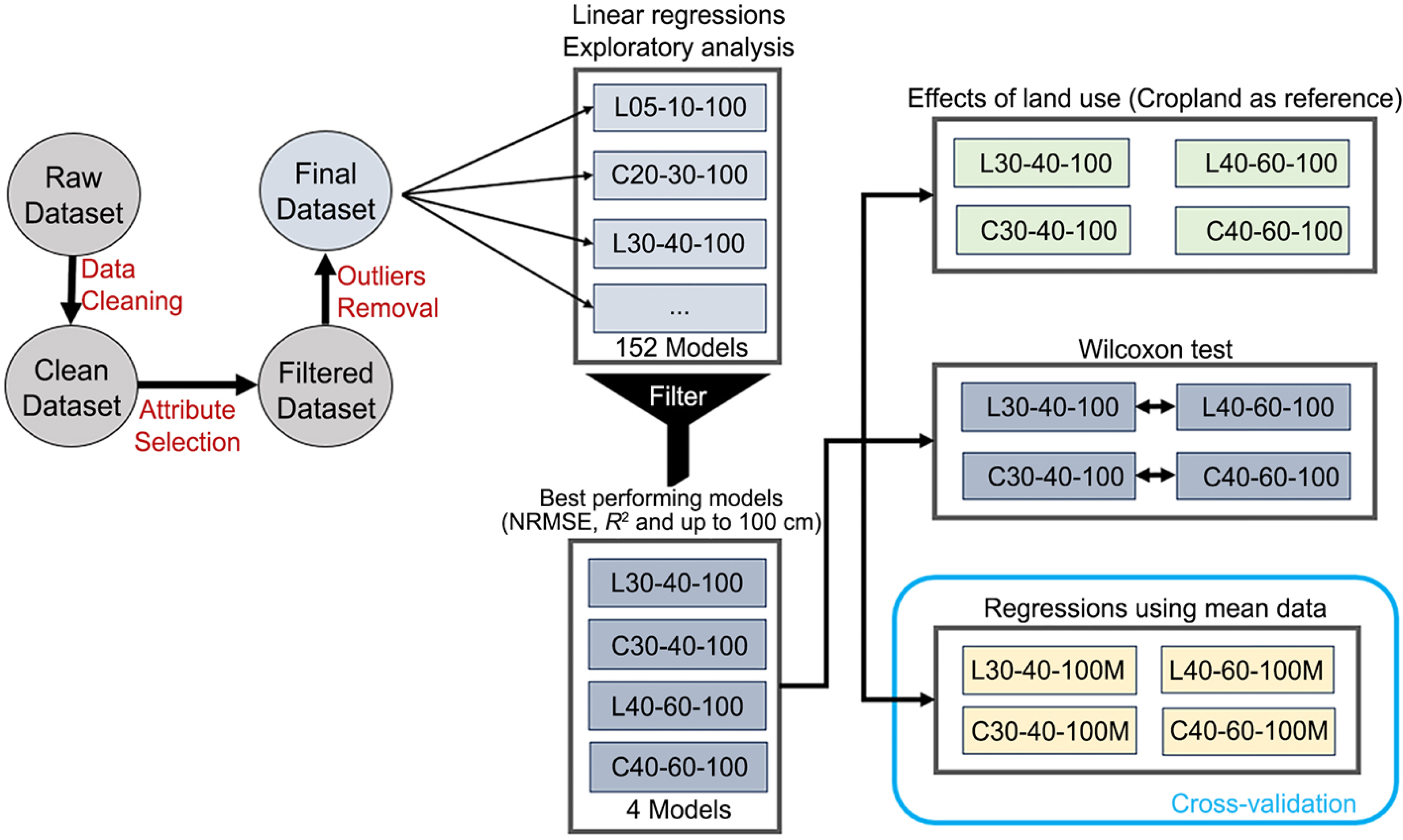
The research progresses through distinct yet interconnected phases. Our analytical workflow, illustrated in Figure 1, outlines the steps from data preparation to model validation. Initially, the raw dataset is cleaned to address inaccuracies and missing values. Subsequently, it is prepared for exploratory analyses.

Figure 1
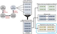
Schematic overview of the data analysis pipeline, illustrating the sequential steps from raw data processing to model validation and cross-validation. Abbreviations: L = laser-induced breakdown spectroscopy; C = carbon, hydrogen, and nitrogen analyzer; suffix M denotes models built using plot-averaged data. NRMSE = normalized root mean square error; R² = coefficient of determination.

During the exploratory phase, 152 candidate models, each based on different combinations of selected predictors, were developed.

Models were selected based on goodness-of-fit statistics and the relevance of available soil information. The selection process applied a filtering criterion that evaluates performance metrics, including normalized root mean square error (NRMSE) and coefficient of determination (R²), while ensuring that the response layer depth encompasses SOC stocks up to the deepest layer (80-100 cm). This filtering narrows the model collection to the four layers that perform best.

Once model selection is complete, our analysis is split into distinct research questions. One approach examines the impact of different land-use types on the model's outcomes, using cropland as the reference category. The second approach evaluates the model's goodness-of-fit for land uses within a specified depth range using the Wilcoxon rank-sum test, a non-parametric test for independent samples. This analysis investigates whether a model that uses less topsoil data compromises predictive accuracy for deeper SOC stocks.

In a practical application of our models for agricultural management, we developed regressions using the mean data, indicated by the ‘M’ suffix in model codes. This approach is particularly relevant because it reflects the real-world scenario in which farm-level estimates are derived from averages of soil or composite samples. To validate the models’ robustness and applicability across various datasets, a 10-fold cross-validation procedure was employed.

Data description

We used soil data collected and made available through the PRO Carbono project, a collaborative research initiative between Embrapa and Bayer Crop Science. This dataset encompasses various soil properties, including physical characteristics (e.g., texture and bulk density), chemical attributes (e.g., pH, carbon content, and nitrogen content), and geographic information (e.g., latitude and longitude) for the soil samples.

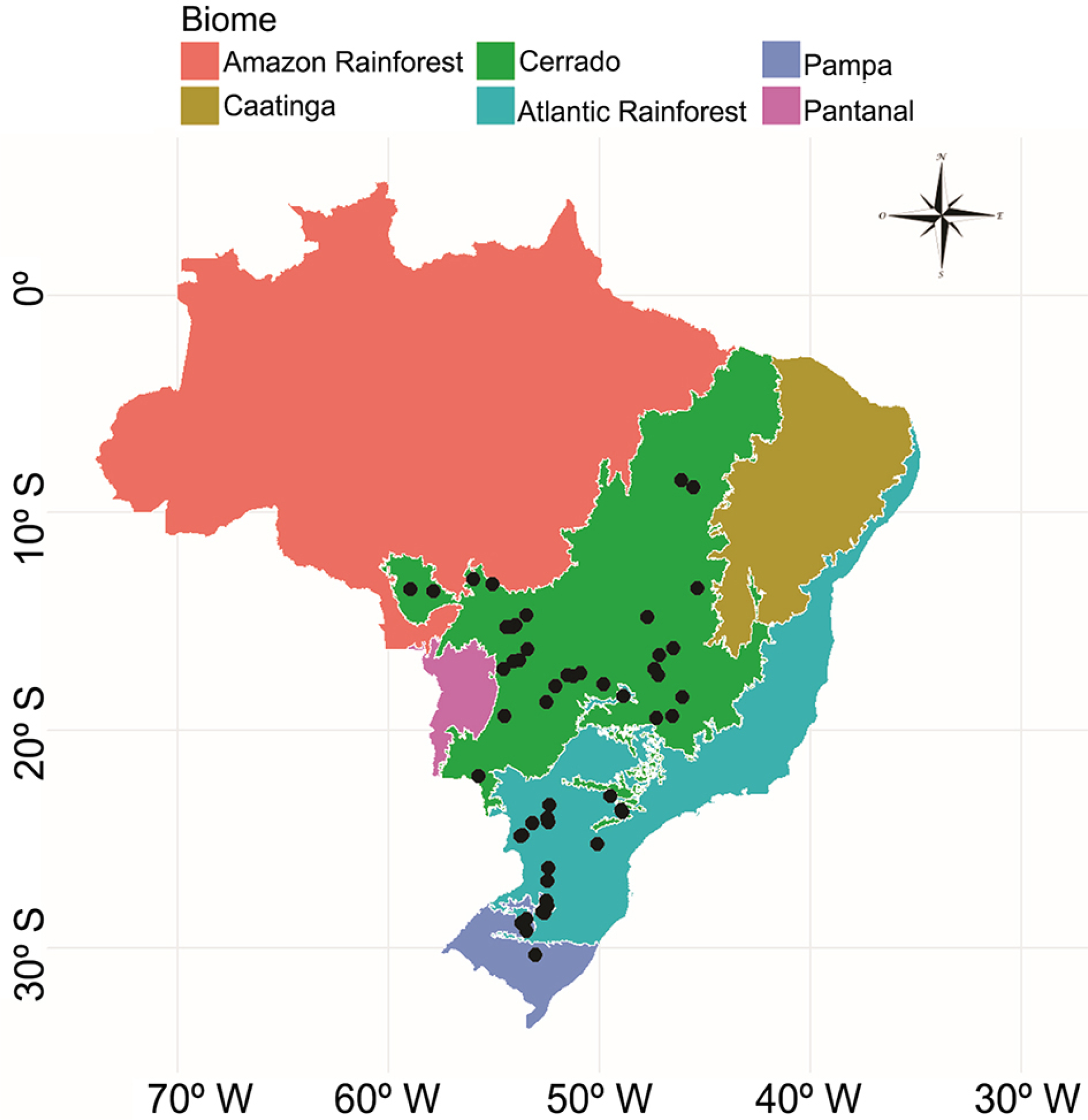
This study analyzed soil samples from 53 farms across Brazil's major biomes, as shown in Figure 2. At each farm, samples were collected from eight trenches in croplands and four trenches in adjacent native vegetation. The croplands primarily featured corn and soybean cultivation. The analysis focused solely on the initial SOC stocks recorded in the project's first year. Due to a lack of longitudinal data, it was not possible to rigorously assess whether the relationships among the layers remain stable over time as SOC stocks fluctuate.

Figure 2
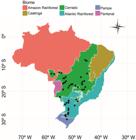
Geographic distribution of farms across major Brazilian biomes. The map showcases farms (depicted as black points) situated within three biomes.

We used SOC data obtained from carbon, hydrogen, and nitrogen method (CHN) (Bredeweg, 1986) that is recognized as the reference method, and laser-induced breakdown spectroscopy (LIBS) (Harmon and Senesi, 2021) that is typically calibrated against it (Poeplau et al., 2017). The dataset underwent thorough cleaning, removing non-essential attributes, those with 60 % or more missing data, and entries from trenches that lacked SOC measurements in deep layers. Consequently, we retained 4,928 LIBS data points and 3,688 CHN data points from the original 5,029. To ensure consistency with the specific land use, we imputed each attribute's average value for the same soil layer and corresponding farm entries.

SOC stocks were determined for each layer using Eq. (1), as described by Poeplau et al. (2017).

(1) $$SOCstoc{k}_{\text{K}}={10}^2\times C_{\text{k}}\times B{D}_{\text{k}}\times d_{\text{k}}$$

where, for layer k, SOCstock_k is the SOC stock (Mg ha⁻¹), C_k is the carbon concentration (g kg⁻¹), BD_k is the bulk density (kg m⁻³), and d_k is the layer thickness (m).

Data treatment

During data processing, we selected key predictive attributes, including soil texture (e.g., clay), pH, nitrogen content, SOC concentration, SOC stocks, and location. We also identified and addressed outliers.

In this study, we employed attribute selection methods to focus on the target SOC stocks in the 60-100 cm depth range, classified as deeper layers. Our decision to investigate this specific depth was based on expert recommendations that sampling up to 60 cm is feasible because it avoids soil compaction and eliminates the need for trench digging.

To estimate SOC stocks in the 60-100 cm depth range from data in the 0-60 cm layers, we evaluated three feature selection methods: CfsSubsetEval, which evaluates subsets based on correlation; CorrelationAttributeEval, which assesses the relevance of individual attributes; and ClassifierSubsetEval, which uses linear regression as a classifier to determine subset importance via performance metrics, specifically root mean square error (RMSE). All methods were implemented in Weka (Witten et al., 2017).

The process of selecting attributes, as described by Kononenko and Hong (1997), is vital for identifying the relevant attributes for modeling the target variable. This selection procedure enhances the model's accuracy, making it easier to implement, interpret, transform, and communicate. After attribute selection, we used scatter plots to visually represent the relationships between the predictor and response variables, thereby enabling us to identify potential correlations.

Three methods were used to identify outliers in the data. A soil profile was classified as an outlier if it met the criteria established by all three methods. The first method (Hoaglin et al., 1986) defines outliers as values that fall outside the lower bound (LB) and upper bound (UB), which are calculated from the interquartile range (IQR), as shown in Eq. (2):

(2) $$LB=Q1-1.5\times IQR\wedge UB=Q3+1.5\times IQR$$

The second method relies on the studentized residual R_i associated with the response y_i from a linear regression model (Eq. 3).

(3) $$R_i=\frac{\widehat{e_i}}{s\times \sqrt{1-h_i}}$$

where $\widehat{e_i}$ and h_i are the residual and leverage for observation i, respectively, and s is the standard deviation of the error e_i. In this method, a data point is considered an outlier if its studentized residual satisfies |R_i| > 3 (Robinson et al., 1984). The third method relies on a linear relationship between the response y_i and a predictor variable x_i of the form y_i = k × x_i, where k remains constant. If this relationship holds, we expect that for each pair of data points (x_i,y_i) the ratio

$$\frac{y_i-x_i}{x_i}$$

should be close to k – 1, as noticed in the relationship given by Eq. (4).

(4) $$\frac{y_i-x_i}{x_i}=\frac{k{x}_i-x_i}{x_i}=\frac{\left(k-1\right)x_i}{x_i}=k-1$$

Significant deviations occur when the ratio defined in Eq. (4) falls below the LB or exceeds the UB, as defined by Eq. (2). Once an observation is identified as an outlier, it is removed from further analysis.

Estimating SOC stocks in deeper layers

Let y_ijk represent the SOC stocks in deeper layers and x_ijk represent the SOC stocks in upper layers, where i = 1,…,n indexes farms, j = 1,2 indexes the land-use type within a given farm, and k = 1,…,m_i indexes the trenches within that land-use type of the farm. The following regression model was defined in Eq. (5).

(5) $$y_{ijk}={\text{β}}_0+{\text{β}}_1{x}_{ijk}+{\text{ε}}_{ijk}$$

where β₀ and β₁ represent the intercept and slope, respectively, and the errors ε_ijk follow a normal distribution with mean 0 and variance σ². Observations (x_ijk, y_ijk) were recorded at specific depth levels, ensuring that the depth associated with the response variable is greater than that of the predictor variable.

The goodness-of-fit of the model was assessed using R² and the NRMSE, which is the RMSE divided by the mean of the observed response variable. While the widely recognized R² value indicates the proportion of the response variable's variability explained by the predictor variable, the NRMSE provides a normalized perspective on the RMSE relative to the response variable magnitude. Lower NRMSE values indicate better model performance. Consequently, optimal model performance is characterized by the highest R² and the lowest NRMSE.

After filtering for optimal models (Figure 1), we proceeded with analyses using the selected models. For that purpose, we replaced y_ijk and x_ijk in Eq. (5) with their averages across the m_i repeated measurements within land use j in farm i, and fitted separate models for CHN and LIBS determinations. Because outliers were removed during preliminary data processing, using averages for modeling is an appropriate complementary approach. Additionally, for our specific objectives, a population-based model is more relevant than a random-effects model. This preference arises from our need to account for the average SOC levels across farms (marginal measures), rather than focusing on variability between individual trenches. This approach enables the assessment of optimal combinations using aggregated farm-level SOC stock data, providing a practical method for carbon quantification and monitoring.

To assess the viability of using a surface layer as a predictor with comparable effectiveness, we conducted a Wilcoxon rank-sum test to determine whether the residuals of top-performing models varied with predictor depth (Wilcoxon, 1945). This nonparametric test was selected for its lack of assumptions about data normality and its effectiveness in comparing independent samples. In our analysis, we examined the residuals of models within the same dataset. Our focus is on gathering comprehensive information on SOC stocks at a lower cost. Consequently, models that predict SOC stocks in deeper layers by leveraging SOC stocks from more economical surface layers are preferred.

Assessment of predictive power using cross-validation

We divided the dataset into ten distinct random folds, each containing a unique subset of data. We then trained the models on nine folds and evaluated their performance on the remaining fold. This process was repeated ten times, with a different fold designated as the test set for each iteration. By averaging the evaluation metrics – R², RMSE, and NRMSE – across all iterations, we obtained a comprehensive assessment of the predictive capability of the fitted models (Efron, 1983). This approach helped mitigate overfitting and provided reliable performance estimates for the models. Consequently, we drew robust conclusions about the models’ suitability for the specific dataset.

Results

Exploratory predictive analysis using linear regression

Attribute selection consistently identified SOC stocks in adjacent upper layers as the most significant predictors, whereas other soil properties, such as clay, sand, silt, pH, bulk density, nitrogen, and longitude, were not retained. Outlier detection showed that fewer than 2 % of profiles exhibited unrealistic deviations between the 40-60 cm and 60-100 cm depths; thus, these points were removed.

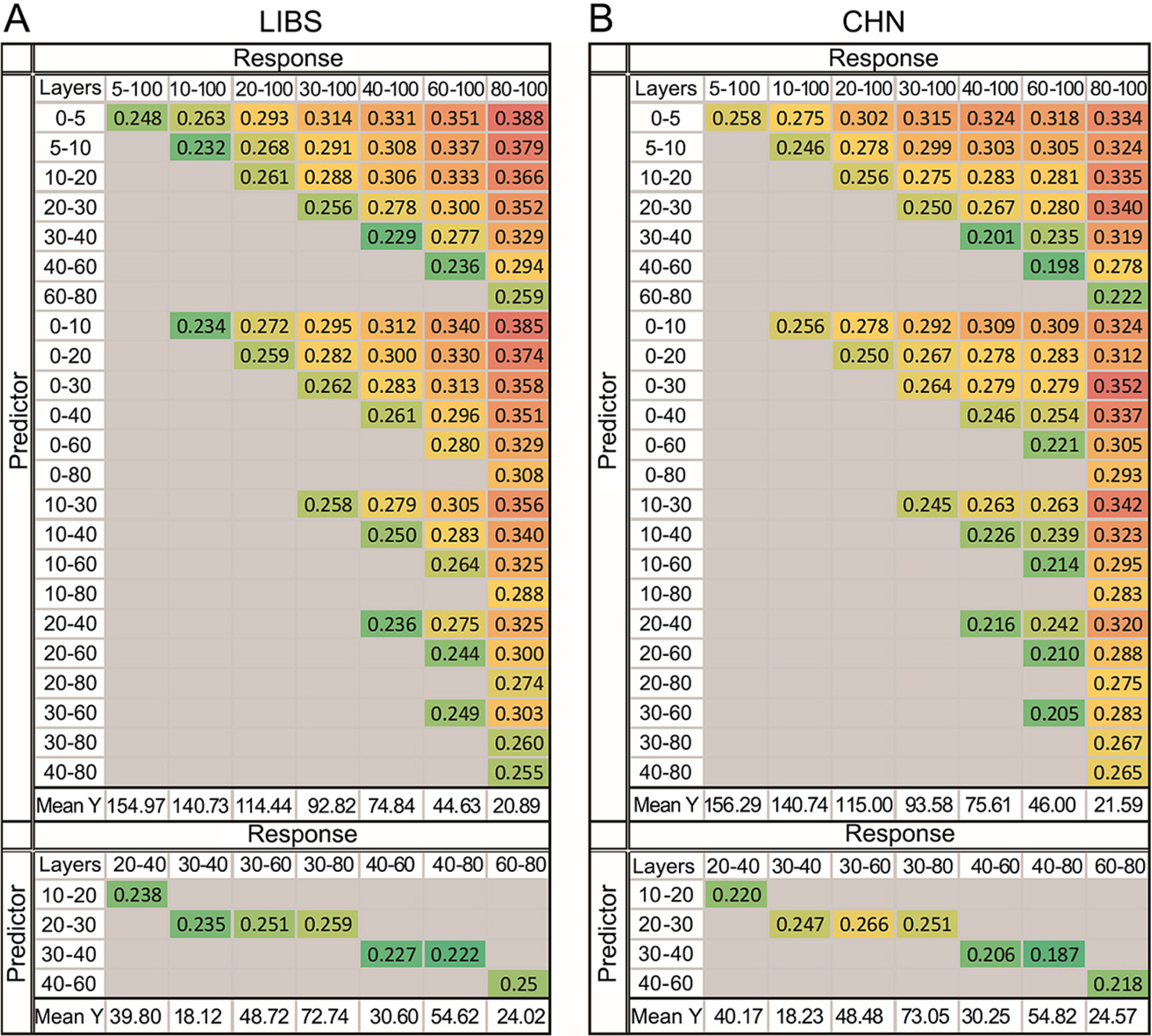
After selecting attributes and removing outliers, regression models were fitted using various combinations of soil layers. The normalized root mean square errors (NRMSEs) for the LIBS and CHN fits are, respectively, shown in Figure 3A-B.

Figure 3
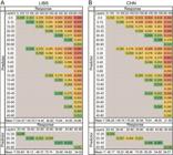
Normalized root mean square error (NRMSE) values for linear regression models using (A) laser-induced breakdown spectroscopy (LIBS), and (B) carbon, hydrogen, and nitrogen analyzer (CHN) data. Each cell shows the NRMSE values for a model with the row as the predictor variable and the column as the response variable. Both variables are soil layers in cm. The row "Mean Y" shows the mean of the response variable for each soil layer.

The results indicated that the most effective models (highest R² and lowest NRMSE) were those that predicted SOC stocks for the 40-100 cm layer based on the 30-40 cm layer, and for the 60-100 cm layer based on the 40-60 cm layer, using both LIBS (Figure 3A) and CHN (Figure 3B) data. Additionally, models that predict SOC stocks within a 1-meter range, such as using the 30-40 cm layer to predict the 40-80 cm layer, also demonstrated considerable effectiveness. However, despite comparable precision, these models provide less comprehensive SOC stock information because they omit deeper layers, such as the 80-100 cm layer.

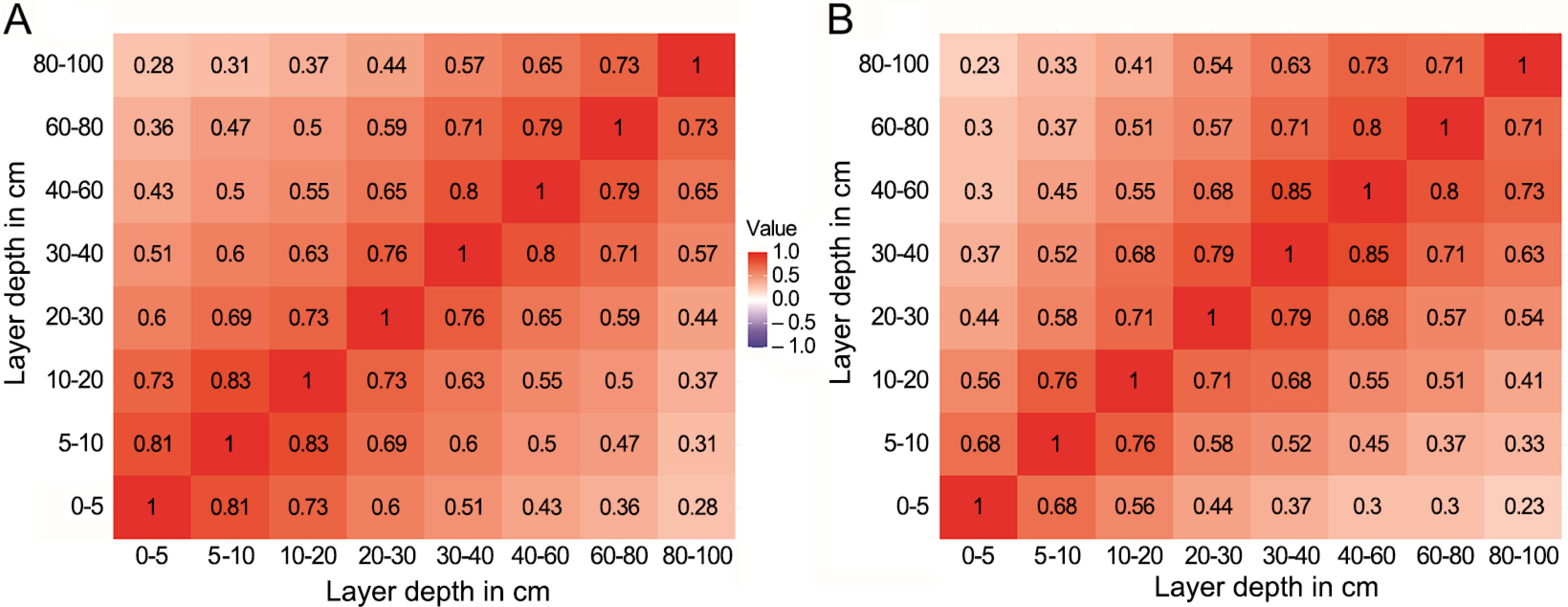
Heatmaps showing the correlation of SOC stocks across depths indicate that correlations are strongest between adjacent layers and decline with increasing distance between layers. For instance, the correlation between the 0-5 cm and 80-100 cm layers is relatively low, with values ranging from 0.23 to 0.28 (Figure 4A-B). In contrast, the correlation between the 30-40 cm and 40-60 cm layers is notably high, with values ranging from 0.80 to 0.85.

Figure 4
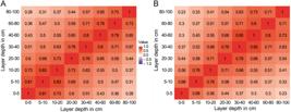
Heatmap comparison of soil organic carbon stock correlations across different soil depths measured by (A) laser-induced breakdown spectroscopy, and (B) carbon, hydrogen, and nitrogen analyzer data.

From this point forward, a labeling scheme based on method and layer depth is used to distinguish the fitted models. The model labels are L30-40-100, L40-60-100, C30-40-100, and C40-60-100. Here, the prefixes ‘L’ and ‘C’ denote the LIBS and CHN methods, respectively. The number following the prefix indicates the depth (cm) at the top of the predictive layer, followed by a dash that separates it from the depth of both the bottom of the predictive layer and the top of the response layer. A second dash precedes the depth at the bottom of the response layer.

The L30-40-100 and C30-40-100 models exhibited high goodness-of-fit, indicating a strong linear relationship between SOC stocks in the 30-40 cm layer and those in the 40-100 cm layer. The R² values for the L30-40-100 and C30-40-100 models were 0.644 and 0.725, respectively, among the highest recorded across all layer combinations and methods evaluated in our study.

In addition to the high-performing L30-40-100 and C30-40-100 models, a comprehensive analysis of other models offers further insight into predictive performance across various soil layers, including the topmost few centimeters. Notably, the L00-10-100 and L05-10-100 models showed surprisingly strong goodness-of-fit, with NRMSE values of 0.234 and 0.232, respectively. In contrast, their counterparts, C00-10-100 and C05-10-100, did not exhibit a similar trend.

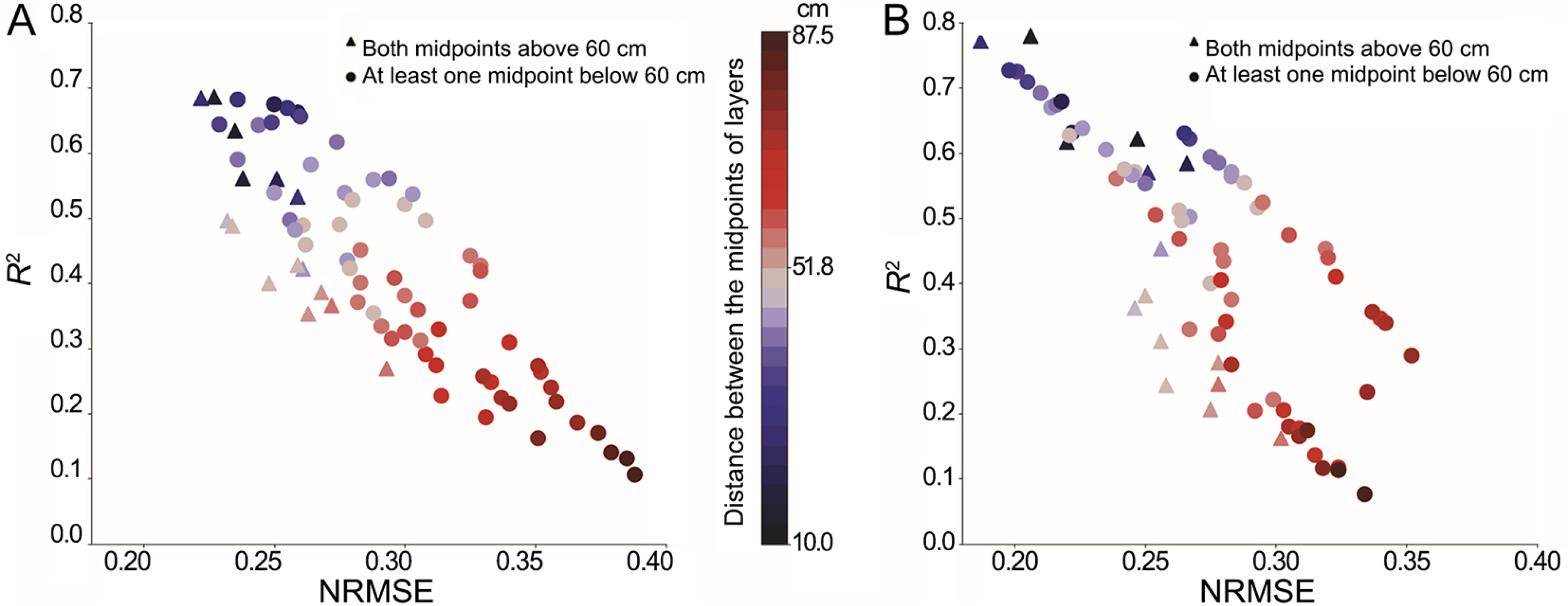
Additionally, we plotted R² scores against NRMSE values for each model (Figure 5A-B). The color gradient on the graph shows the distance between the midpoints of the predictor and response soil layers, ranging from dark blue to dark red, corresponding to the smallest (10 cm) and largest (87.5 cm) distances investigated, respectively. The results indicate a correlation of the distance between the predictor and response layer midpoints and an increase in NRMSE values.

Figure 5
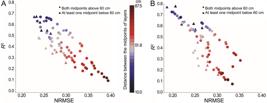
Relationship between normalized root mean square error (NRMSE) and coefficient of determination (R²) with (A) laser-induced breakdown spectroscopy, and (B) carbon, hydrogen, and nitrogen analyzer data. The colormap indicates the distance between the midpoints of the predictor and response layers. The triangle symbol represents points where the midpoints of the predictor and response layers are above 60 cm, while the circle symbol represents points where at least the midpoint of either layer or both layers is below 60 cm.

Further analysis indicated that the increase in NRMSE was not consistent across all distances. Specifically, NRMSE values were well correlated with distances within the 2.5 - 35 cm range, but increased beyond that range. We categorized the data based on whether the midpoints of both the predictor and response variables exceeded 60 cm. This classification, illustrated in Figure 5A-B, aimed to ensure comparable sample sizes within each category after the data split. These figures indicate that the greater variability in SOC stocks typically found in the upper layers often results in lower R² values for the models. Notably, this reduction in R² occurs when NRMSE remains relatively constant, and the distance between the midpoints of the predictive and response layers is similar.

Comparison of best-performing models

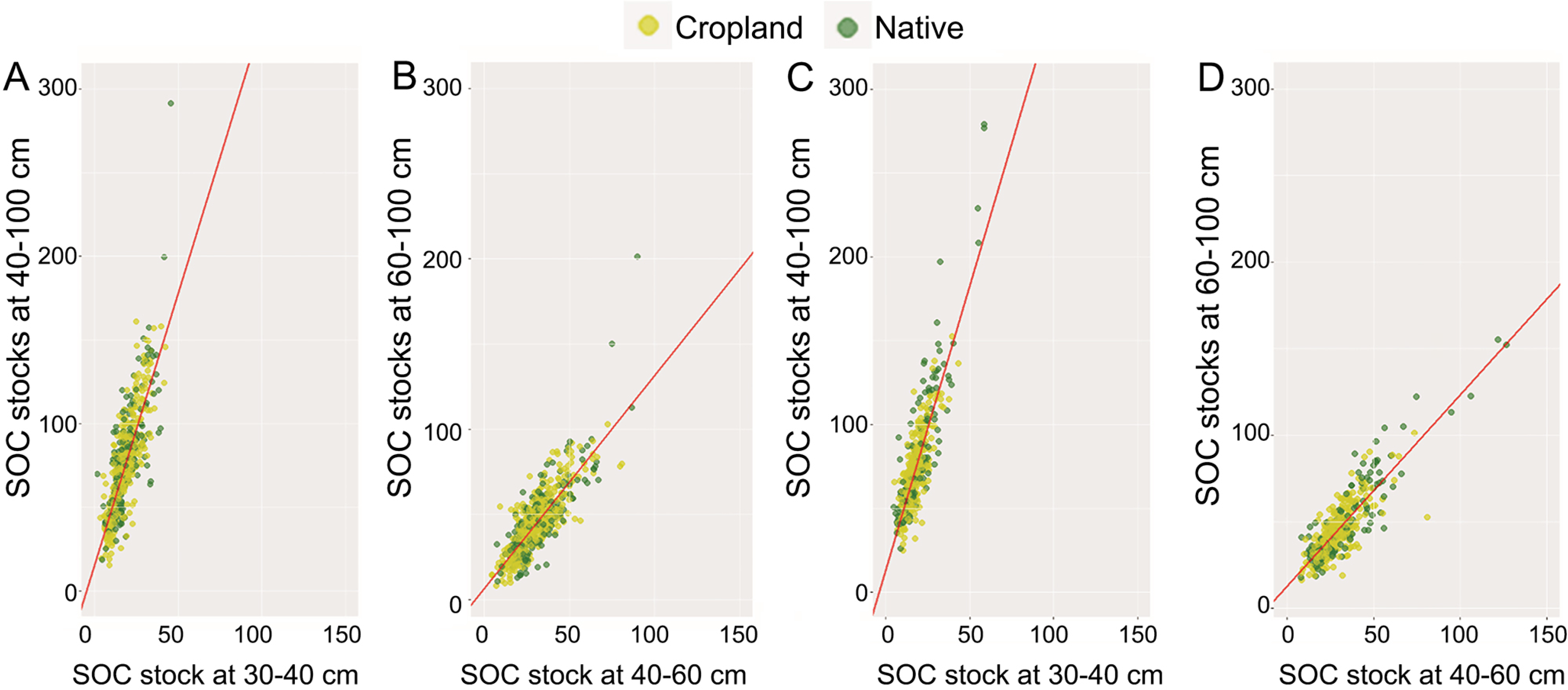
The four best-performing models: L30-40-100, L40-60-100, C30-40-100, and C40-60-100 are presented in Figure 6A-D. Comparing the models in Figure 6, the models in Figure 6A and 6C show a steeper slope. The pronounced upward trajectory indicates that SOC stocks at 30-40 cm are substantially linearly correlated with those at 40-100 cm. In contrast, the fitted lines for the other two models (Figure 6B and D) exhibit a less pronounced slope, suggesting more stable SOC stocks within this depth interval.

Figure 6
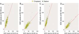
Scatter plots of soil organic carbon (SOC) stocks at different depths for (A and B) laser-induced breakdown spectroscopy, and (C and D) carbon, hydrogen, and nitrogen analyzer, with linear regression fit (red line).

In all models, the fitted regression line effectively captures most data points within a relatively narrow band. However, the band of predicted values is significantly narrower in the L30-40-100 and C30-40-100 models.

Estimates for the intercept and slope, RMSE, NRMSE, R², and the sample mean of the response layer ($\overline{Y}$) for models L30-40-100, L40-60-100, C30-40-100, and C40-60-100 are presented in Table 1. The L30-40-100 and C30-40-100 models exhibit similar intercepts and slopes across the carbon quantification methods, whereas the L40-60-100 and C40-60-100 models show notable differences in both intercepts and slopes. NRMSE values are relatively low across all models, ranging from 0.198 to 0.236, with LIBS models slightly higher than CHN models. Additionally, the RMSE is lower for the L40-60-100 and C40-60-100 models than for the L30-40-100 and C30-40-100 models, respectively, consistent with the understanding that the mean SOC stocks at depth are lower for the former models than for the latter.

Table 1
Linear regression estimates, root mean square error (RMSE), normalized root mean square error (NRMSE) for the four tested models, coefficient of determination (R²) and sample mean of response layer ($\overline{Y}$) for models L30-40-100, L40-60-100, C30-40-100 and C40-60-100.

Model	Intercept	Slope	RMSE	NRMSE	R 2	$\overline{Y}$
L30-40-100	16.30 ± 1.91	3.25 ± 0.10	17.24	0.229	0.64	75.14
L40-60-100	6.93 ± 1.14	1.25 ± 0.03	10.66	0.236	0.68	45.17
C30-40-100	14.43 ± 1.93	3.38 ± 0.10	15.34	0.201	0.72	76.19
C40-60-100	13.09 ± 1.05	1.11 ± 0.03	9.21	0.198	0.73	46.22

• The value after ± is the standard error of the estimate. L = laser-induced breakdown spectroscopy; C = carbon, hydrogen, and nitrogen analyzer.

We tested the null hypothesis that there was no statistically significant difference in the response variable across land uses within each of the best-performing models. Our analysis did not lead to rejection of the null hypothesis, indicating that there is no significant difference among land-use types in the L30-40-100 and C40-60-100 models. However, we observed a significant difference between cropland and native models for L40-60-100 and C30-40-100. The p-values associated with the interaction terms involving native areas, with croplands as the reference category, are shown in Table 2.

Table 2
Interaction effects of native areas on each linear regression model (using cropland as reference).

Model	Interaction on intercept	p-value	Interaction on slope	p-value
L30-40-100	1.992	0.616	–0.066	0.743
L40-60-100	–6.615	0.006	0.190	0.007
C30-40-100	–11.385	0.004	0.823	< 0.001
C40-60-100	–3.328	0.140	0.117	0.082

• L = laser-induced breakdown spectroscopy; C = carbon, hydrogen, and nitrogen analyzer.

Furthermore, the Wilcoxon rank-sum test was used to assess the significance of differences in residual distributions across comparable models within the two groups, LIBS and CHN. Specifically, we compared the residuals of models L30-40-100 and L40-60-100 to evaluate their performance in predicting SOC stocks within their respective depth ranges. Similarly, we compared the models C30-40-100 and C40-60-100. The results indicated that the differences in residuals for the LIBS models (L30-40-100 vs. L40-60-100) were not statistically significant, with a p-value of 0.329 (0.9241 after standardizing the residuals). Likewise, the residuals for the CHN models (C30-40-100 vs. C40-60-100) showed no statistically significant difference, with p-values of 0.230 (0.4721 after standardizing the residuals).

We subsequently performed linear regression analyses using the mean data for each land-use type across farms to predict SOC stocks within specific depth ranges. The models developed include L30-40-100M, L40-60-100M, C30-40-100M, and C40-60-100M. These models provide a practical approach to predicting SOC stocks that is consistent with standard field sampling and measurement practices while maintaining predictive accuracy. All models using the LIBS and CHN mean data demonstrate strong predictive power, with R² values ranging from 0.82 to 0.89. Both LIBS and CHN methods yield comparable NRMSE values of approximately 0.12-0.15 throughout the analysis, although models incorporating LIBS data exhibit higher RMSE values than those based on CHN data. The results of this linear regression analysis, including the R², NRMSE, and RMSE, are presented in Table 3.

Table 3
Linear regression models with mean data performance coefficients.

Model	RMSE	R 2	NRMSE
L30-40-100M	11.00	0.82	0.15
L40-60-100M	6.47	0.85	0.14
C30-40-100M	9.54	0.89	0.12
C40-60-100M	6.61	0.84	0.14

• RMSE = root mean square error; NRMSE = normalized root mean square error; R² = coefficient of determination; L = laser-induced breakdown spectroscopy; C = carbon, hydrogen, and nitrogen analyzer; suffix M denotes models built using plot-averaged data.

Residual analysis revealed no evidence of heteroscedasticity or trends. Furthermore, the regression models showed no deviations from normality. The 10-fold cross-validation provided valuable insights into the models’ generalization and performance on unseen data. A comparison of the LIBS and CHN methods indicates that both techniques perform similarly across various soil depths (Table 4). The calculated RMSE ranges from 6.40 to 11.10, while the R² values range from 0.82 to 0.87. Additionally, the NRMSE for the CHN data ranges from 0.125 to 0.146, compared with 0.141 to 0.148 for LIBS data.

Table 4
Ten-fold cross-validation results for root mean square error (RMSE), coefficient of determination (R²), and normalized root mean square error (NRMSE) for the four tested models.

Model	RMSE	R 2	NRMSE
L30-40-100M	11.10 ± 1.97	0.83 ± 0.09	0.148
L40-60-100M	6.40 ± 1.72	0.87 ± 0.07	0.141
C30-40-100M	9.53 ± 3.46	0.84 ± 0.14	0.125
C40-60-100M	6.73 ± 2.04	0.82 ± 0.13	0.146

• L = laser-induced breakdown spectroscopy; C = carbon, hydrogen, and nitrogen analyzer; suffix M denotes models built using plot-averaged data.

Discussion

Our findings suggest that near-surface measurements, already included in standard MRV programs, can accurately estimate deeper carbon reserves. This has important implications for developing affordable, scalable protocols to support carbon farming initiatives in Brazil.

The proportion of SOC stocks in deeper layers is comparable to that observed in tropical climates. For instance, a mean SOC stock of 37.87 Mg ha⁻¹ in the 20-40 cm layer has been reported in tropical Andisols (Veldkamp, 1994), and one-third of the SOC stocks have been found below 50 cm within 1 meter (Nottingham et al., 2020). These findings challenge existing assumptions about SOC distribution and underscore the significant carbon sequestration potential of deeper soil layers, particularly in tropical regions, where SOC proportions at depth often exceed those in temperate regions (Trumbore, 1993; Jobbágy and Jackson, 2000; Stone and Plante, 2015).

Quantifying and monitoring the maintenance of sufficient SOC stocks in deeper cropland layers is crucial, given the potential for significant changes in these stocks. Long-term experiments in Germany, spanning from 32 to 112 years, have shown that approximately one-fifth of agriculture-related changes in SOC stocks occur in the subsoil (30-100 cm) (Skadell et al., 2023). Similarly, a study conducted in Brazil found that half of the changes in SOC stocks occurred within the same subsoil range (Veloso et al., 2018). Protocols, such as those established by the Intergovernmental Panel on Climate Change (IPCC), recommend soil sampling to a depth of 30 cm; however, this approach can underestimate SOC stocks by as much as 60 % and ecosystem carbon by 30 % (Wade et al., 2019). Consequently, failing to quantify subsoil SOC stocks may lead to inaccurate assessments of changes in these stocks, undermining the effectiveness of climate change mitigation efforts.

Although SOC dynamics are complex and vary with depth, influenced by factors such as microbiological composition, root distribution, and gas diffusion (Lorenz and Lal, 2005; Lockhart et al., 2023; Souza et al., 2023), the predictive relationship between surface and deeper stocks remains robust. In particular, tropical and subtropical soils, such as those found in Brazil, exhibit unique mineralogical characteristics, namely a clay fraction dominated by kaolinite and low-crystallinity Fe and Al oxides, which favor the effective stability of soil organic matter (SOM) (Rodríguez-Albarracín et al., 2023). This may help explain the observed correlation between surface and deeper SOC stocks, though further investigation is warranted.

Regression models may not fully capture complex interactions among processes such as organic matter decomposition, root exudation, rainfall, percolation, and soil physicochemical properties that influence soil dynamics. Nevertheless, they remain valuable for examining SOC stocks across various soil layers (Matus, 2021). Our regression analysis indicates that SOC stocks in adjacent soil layers are most strongly correlated (Figure 4A-B). Interestingly, increasing the depth of the predictor layer does not necessarily improve predictive power. This suggests that the lower boundary of the topsoil (30-40 cm) consistently serves as an effective predictor of deeper SOC stocks, outperforming upper layers and even showing stronger predictive capability than when combined with deeper layers. Moreover, selecting predictor variables more closely associated with the response variable, particularly those within 35 cm, does not automatically yield more accurate predictions.

The Wilcoxon rank-sum test showed that the models L30-40-100 and C30-40-100 performed comparably to the models L40-60-100 and C40-60-100. These findings are further supported by residual analysis, which confirmed the robustness of the regression models and indicated adherence to assumptions of homoscedasticity, independence, and normality. The R² values from the mean models (Table 3) indicate a strong correlation between actual measurements and predicted SOC stocks, highlighting the suitability of both methods for accurate soil carbon assessment. This is particularly noteworthy given that standard field practices typically involve calculating the average value of soil samples within relatively uniform areas (Ravindranath and Ostwald, 2008). Moreover, the NRMSE analysis (Table 3) indicates that the prediction errors of both models relative to the mean value of soil carbon content are fairly consistent.

Our findings underscore the significant potential of the 30-40 cm layer as an effective predictor of the 40-100 cm layer (Figure 6A-D), accounting for a significant share of the variance observed in deeper layers. This is particularly notable because measuring the 30-40 cm layer can be seamlessly integrated into standard MRV practices. Therefore, implementing these models requires no additional effort or modifications to existing protocols, making them both effective and highly practical for routine carbon soil assessments. Furthermore, the correlation between SOC stocks at 30-40 cm and 40-100 cm remains consistent across various measurement techniques. However, this level of consistency is not observed in other well-fitted models, such as L40-60-100 and C40-60-100.

The regression models presented in this study effectively predict deeper SOC stocks with a reasonable margin of error. These findings have practical implications for expanding carbon markets. Accurate SOC stock predictions can substantially reduce sampling costs for farmers, enabling more efficient monitoring and identification of carbon sequestration at the farm level. This can be converted into carbon credits, providing a financial incentive for landowners and farmers to adopt practices that enhance SOC sequestration. Moreover, the carbon market enables corporations and governments to meet their carbon-reduction targets by investing in carbon projects that promote sustainable land management and combat climate change.

Recognizing the limitations of sample quality and diversity is crucial, especially in Brazil's diverse agricultural landscape. Although our dataset is the most comprehensive collection of soil organic carbon (SOC) data in Brazil, its representativeness could be further enhanced by incorporating topographic and climatic factors and by focusing on underrepresented regions to improve model accuracy. Optimizing deeper SOC requires a careful balance between carbon sequestration and soil capacity. Quantifying SOC is complex, encompassing both quantity and quality, which are influenced by spatiotemporal molecular diversity and land-use and management changes. While our study provides valuable insights into predicting static SOC stocks in deeper layers, future research should expand this modeling approach to assess its effectiveness in predicting changes in deeper SOC stocks driven by sustainable and regenerative practices and changing climate patterns.

• Declaration of use of AI Technologies
  The authors used "ChatGPT-4.0" and "Gemini Advanced" to improve the text (grammar, coherence, and cohesion) and LaTeX formatting.

Acknowledgments

This work was conducted and supported in the framework of PRO Carbono, a collaborative research project between Embrapa and Bayer Crop Science. The third author thanks the Royal Society Wolfson Visiting Fellowships for the research grant (RSWVF\R2\222008). The fourth author thanks Fundação de Amparo à Pesquisa do Estado de São Paulo (FAPESP) for the research grant (2022/08629-4).

Data Availability Statement

The data that support the findings of this study are confidential and proprietary and therefore not publicly available.

References

• Bredeweg RL. 1986. Carbon, hydrogen, and nitrogen analyzer: US Patent No. 4622009. Washington, DC, USA.
• Brummitt CD, Mathers CA, Keating RA, O'Leary K, Easter M, Friedl MA, et al. 2024. Solutions and insights for agricultural monitoring, reporting, and verification (MRV) from three consecutive issuances of soil carbon credits. Journal of Environmental Management 369: 122284. https://doi.org/10.1016/j.jenvman.2024.122284
  » https://doi.org/10.1016/j.jenvman.2024.122284
• Cerri CEP, Damian JM, Alves PA, Cerri DGP, Cherubin MR. 2024. On-farm greenhouse gas emissions and soil carbon stocks of a soybean-maize system. Nutrient Cycling in Agroecosystems 128: 309-324. https://doi.org/10.1007/s10705-024-10356-7
  » https://doi.org/10.1007/s10705-024-10356-7
• Clivot H, Mouny J-C, Duparque A, Dinh J-L, Denoroy P, Houot S, et al. 2019. Modeling soil organic carbon evolution in long-term arable experiments with AMG model. Environmental Modelling & Software 118: 99-113. https://doi.org/10.1016/j.envsoft.2019.04.004
  » https://doi.org/10.1016/j.envsoft.2019.04.004
• Davis MR, Alves BJR, Karlen DL, Kline KL, Galdos M, Abulebdeh D. 2018. Review of soil organic carbon measurement protocols: A US and Brazil comparison and recommendation. Sustainability 10: 53. https://doi.org/10.3390/su10010053
  » https://doi.org/10.3390/su10010053
• Efron B. 1983. Estimating the error rate of a prediction rule: Improvement on cross- validation. Journal of the American Statistical Association 78: 316-331. https://doi.org/10.1080/01621459.1983.10477973
  » https://doi.org/10.1080/01621459.1983.10477973
• Georgiou K, Jackson RB, Vindušková O, Abramoff RZ, Ahlström A, Feng W, et al. 2022. Global stocks and capacity of mineral-associated soil organic carbon. Nature Communications 13: 3797. https://doi.org/10.1038/s41467-022-31540-9
  » https://doi.org/10.1038/s41467-022-31540-9
• Geremew B, Tadesse T, Bedadi B, Gollany HT, Tesfaye K, Aschalew A, et al. 2024. Evaluation of RothC model for predicting soil organic carbon stock in north-west Ethiopia. Environmental Challenges 15: 100909. https://doi.org/10.1016/j.envc.2024.100909
  » https://doi.org/10.1016/j.envc.2024.100909
• Gomiero T. 2019. Soil and crop management to save food and enhance food security. Saving Food 2: 33-87. https://doi.org/10.1016/B978-0-12-815357-4.00002-X
  » https://doi.org/10.1016/B978-0-12-815357-4.00002-X
• Gross CD, Harrison RB. 2019. The case for digging deeper: Soil organic carbon storage, dynamics, and controls in our changing world. Soil Systems 3: 28. https://doi.org/10.3390/soilsystems3020028
  » https://doi.org/10.3390/soilsystems3020028
• Harmon RS, Senesi GS. 2021. Laser-induced breakdown spectroscopy - A geochemical tool for the 21st century. Applied Geochemistry 128: 104929. https://doi.org/10.1016/j.apgeochem.2021.104929
  » https://doi.org/10.1016/j.apgeochem.2021.104929
• Hoaglin DC, Iglewicz B, Tukey JW. 1986. Performance of some resistant rules for outlier labeling. Journal of the American Statistical Association 81: 991-999. https://doi.org/10.1080/01621459.1986.10478363
  » https://doi.org/10.1080/01621459.1986.10478363
• Jandl R, Rodeghiero M, Martinez C, Cotrufo MF, Bampa F, van Wesemael B, et al. 2014. Current status, uncertainty and future needs in soil organic carbon monitoring. Science of The Total Environment 468-469: 376-383. https://doi.org/10.1016/j.scitotenv.2013.08.026
  » https://doi.org/10.1016/j.scitotenv.2013.08.026
• Jobbágy EG, Jackson RB. 2000. The vertical distribution of soil organic carbon and its relation to climate and vegetation. Ecological Applications 10: 423-436. https://doi.org/10.1890/1051-0761(2000)010[0423:TVDOSO]2.0.CO;2
  » https://doi.org/10.1890/1051-0761(2000)010[0423:TVDOSO]2.0.CO;2
• Kononenko I, Hong SJ. 1997. Attribute selection for modelling. Future Generation Computer Systems 13: 181-195. https://doi.org/10.1016/S0167-739X(97)81974-7
  » https://doi.org/10.1016/S0167-739X(97)81974-7
• Lockhart SRA, Keller CK, Evans RD, Carpenter-Boggs LA, Huggins DR. 2023. Soil CO2 in organic and no-till agroecosystems. Agriculture, Ecosystems and Environment 349: 108442. https://doi.org/10.1016/j.agee.2023.108442
  » https://doi.org/10.1016/j.agee.2023.108442
• Lorenz K, Lal R. 2005. The depth distribution of soil organic carbon in relation to land use and management and the potential of carbon sequestration in subsoil horizons. Advances in Agronomy 88: 35-66. https://doi.org/10.1016/S0065-2113(05)88002-2
  » https://doi.org/10.1016/S0065-2113(05)88002-2
• Matus FJ. 2021. Fine silt and clay content is the main factor defining maximal C and N accumulations in soils: a meta-analysis. Scientific Reports 11: 6438. https://doi.org/10.1038/s41598-021-84821-6
  » https://doi.org/10.1038/s41598-021-84821-6
• Nottingham AT, Meir P, Velasquez E, Turner BL. 2020. Soil carbon loss by experimental warming in a tropical forest. Nature 584: 234-237. https://doi.org/10.1038/s41586-020-2566-4
  » https://doi.org/10.1038/s41586-020-2566-4
• Oelkers EH, Cole DR. 2008. Carbon dioxide sequestration: A solution to a global problem. Elements 4: 305-310. https://doi.org/10.2113/gselements.4.5.305
  » https://doi.org/10.2113/gselements.4.5.305
• Paustian K, Lehmann J, Ogle S, Reay D, Robertson GP, Smith P. 2016. Climate-smart soils. Nature 532: 49-57. https://doi.org/10.1038/nature17174
  » https://doi.org/10.1038/nature17174
• Plaza-Bonilla D, Álvaro-Fuentes J, Cantero-Martínez C. 2014. Identifying soil organic carbon fractions sensitive to agricultural management practices. Soil and Tillage Research 139: 19-22. https://doi.org/10.1016/j.still.2014.01.006
  » https://doi.org/10.1016/j.still.2014.01.006
• Poeplau C, Vos C, Don A. 2017. Soil organic carbon stocks are systematically overestimated by misuse of the parameters bulk density and rock fragment content. Soil 3: 61-66. https://doi.org/10.5194/soil-3-61-2017
  » https://doi.org/10.5194/soil-3-61-2017
• Raihan A, Begum RA, Nizam M, Said M, Pereira JJ. 2022. Dynamic impacts of energy use, agricultural land expansion, and deforestation on CO2 emissions in Malaysia. Environmental and Ecological Statistics 29: 477-507. https://doi.org/10.1007/s10651-022-00532-9
  » https://doi.org/10.1007/s10651-022-00532-9
• Ravindranath NH, Ostwald M. 2008. Carbon Inventory Methods: Handbook for Greenhouse Gas Inventory, Carbon Mitigation and Roundwood Production Projects. Springer Springer Dordrecht 1: 306. https://doi.org/10.1007/978-1-4020-6547-7
  » https://doi.org/10.1007/978-1-4020-6547-7
• Robinson A, Cook RD, Weisberg S. 1984. Residuals and influence in regression. Journal of the Royal Statistical Society. Series A (General) 147: 108. https://doi.org/10.2307/2981746
  » https://doi.org/10.2307/2981746
• Rodríguez-Albarracín HS, Demattê JAM, Rosin NA, Contreras AED, Silvero NEQ, Cerri CEP, et al. 2023. Potential of soil minerals to sequester soil organic carbon. Geoderma 436: 116549. https://doi.org/10.1016/j.geoderma.2023.116549
  » https://doi.org/10.1016/j.geoderma.2023.116549
• Rumpel C, Kögel-Knabner I. 2011. Deep soil organic matter - a key but poorly understood component of terrestrial C cycle. Plant and Soil 338: 143-158. https://doi.org/10.1007/s11104-010-0391-5
  » https://doi.org/10.1007/s11104-010-0391-5
• Silva RO, Barioni LG, Pellegrino GQ, Moran D. 2018. The role of agricultural intensification in Brazil's nationally determined contribution on emissions mitigation. Agricultural Systems 161: 102-112. https://doi.org/10.1016/j.agsy.2018.01.003
  » https://doi.org/10.1016/j.agsy.2018.01.003
• Skadell LE, Schneider F, Gocke MI, Guigue J, Amelung W, Bauke SL, et al. 2023. Twenty percent of agricultural management effects on organic carbon stocks occur in subsoils- results of ten long-term experiments. Agriculture, Ecosystems and Environment 356: 108619. https://doi.org/10.1016/j.agee.2023.108619
  » https://doi.org/10.1016/j.agee.2023.108619
• Souza LFT, Hirmas DR, Sullivan PL, Reuman DC, Kirk MF, Li L, et al. 2023. Root distributions, precipitation, and soil structure converge to govern soil organic carbon depth distributions. Geoderma 437: 116569. https://doi.org/10.1016/j.geoderma.2023.116569
  » https://doi.org/10.1016/j.geoderma.2023.116569
• Stone MM, Plante AF. 2015. Relating the biological stability of soil organic matter to energy availability in deep tropical soil profiles. Soil Biology and Biochemistry 89: 162-171. https://doi.org/10.1016/j.soilbio.2015.07.008
  » https://doi.org/10.1016/j.soilbio.2015.07.008
• Tripathi S, Srivastava P, Devi RS, Bhadouria R. 2020. Influence of synthetic fertilizers and pesticides on soil health and soil microbiology. p. 25-54. In: Prasad MNV. ed. Agrochemicals detection, treatment and remediation. Butterworth-Heinemann, Oxford, UK. https://doi.org/10.1016/B978-0-08-103017-2.00002-7
  » https://doi.org/10.1016/B978-0-08-103017-2.00002-7
• Trumbore SE. 1993. Comparison of carbon dynamics in tropical and temperate soils using radiocarbon measurements. Global Biogeochemical Cycles 7: 275-290. https://doi.org/10.1029/93GB00468
  » https://doi.org/10.1029/93GB00468
• Veldkamp E. 1994. Organic carbon turnover in three tropical soils under pasture after deforestation. Soil Science Society of America Journal 58: 175-180. https://doi.org/10.2136/sssaj1994.03615995005800010025x
  » https://doi.org/10.2136/sssaj1994.03615995005800010025x
• Veloso MG, Angers DA, Tiecher T, Giacomini S, Dieckow J, Bayer C. 2018. High carbon storage in a previously degraded subtropical soil under no-tillage with legume cover crops. Agriculture, Ecosystems and Environment 268: 15-23. https://doi.org/10.1016/j.agee.2018.08.024
  » https://doi.org/10.1016/j.agee.2018.08.024
• Wade AM, Richter DD, Medjibe VP, Bacon AR, Heine PR, White LJT, et al. 2019. Estimates and determinants of stocks of deep soil carbon in Gabon, Central Africa. Geoderma 341: 236-248. https://doi.org/10.1016/j.geoderma.2019.01.004
  » https://doi.org/10.1016/j.geoderma.2019.01.004
• Wilcoxon F. 1945. Individual comparisons by ranking methods. Biometrics Bulletin 1: 80-83. https://doi.org/10.2307/3001968
  » https://doi.org/10.2307/3001968
• Witten IH, Frank E, Hall MA, Pal CJ. 2017. Data Mining: Practical Machine Learning Tools and Techniques. 4ed. Morgan Kaufmann, San Francisco, CA, USA. https://doi.org/10.1016/C2015-0-02071-8
  » https://doi.org/10.1016/C2015-0-02071-8
• Xu X, Du C, Ma F, Shen Y, Zhou J. 2019. Fast and simultaneous determination of soil properties using laser-induced breakdown spectroscopy (LIBS): A case study of typical farmland soils in China. Soil Systems 3: 66. https://doi.org/10.3390/soilsystems3040066
  » https://doi.org/10.3390/soilsystems3040066
• Yang X-M, Wander MM. 1999. Tillage effects on soil organic carbon distribution and storage in a silt loam soil in Illinois. Soil and Tillage Research 52: 1-9. https://doi.org/10.1016/S0167-1987(99)00051-3
  » https://doi.org/10.1016/S0167-1987(99)00051-3
• Young MD, Ros GH, Vries W. 2021. Impacts of agronomic measures on crop, soil, and environmental indicators: a review and synthesis of meta-analysis. Agriculture, Ecosystems and Environment 319: 107551. https://doi.org/10.1016/j.agee.2021.107551
  » https://doi.org/10.1016/j.agee.2021.107551
• Zhuang Q, Shao Z, Kong L, Huang X, Li Y, Yan Y, et al. 2023. Assessing the effects of agricultural management practices and land-use changes on soil organic carbon stocks. Soil and Tillage Research 231: 105716. https://doi.org/10.1016/j.still.2023.105716
  » https://doi.org/10.1016/j.still.2023.105716

Edited by

• Edited by:
  Luiz Alexandre Peternelli https://orcid.org/0000-0002-7683-0583

Publication Dates

• Publication in this collection
  17 July 2026
• Date of issue
  2026

History

• Received
  23 June 2025
• Accepted
  21 Sept 2025