Application of computational fluid dynamics on a study in swine facilities with mechanical ventilation system

ABSTRACT:

Ventilation systems used in swine facilities deserve to be studied because they directly affect productivity in the pig farming sector. Bearing this in mind the uniformity of air distribution and temperature is essential to animal welfare in this breeding environment. Thus, the purpose of this study was to identify whether changes in air entrances and exhaust fan positioning could influence air velocity and temperature distribution. The experimental data were collected in a commercial full-scale sow facility. Validation was carried out by comparing the simulated air temperatures and data measured in the field. These results showed agreement between data with a maximum relative error of approximately 3 %. The real settings showed a gradual increase in the air velocity from the air entrances and dead zones due to the change in airflow direction. There was no difference when the positioning of the exhaust fans was altered or was maintained in the original air entrances. The proposed arrangement with only one air inlet reduced the areas of low air movement as a consequence of the change in flow direction. Furthermore, the variables have the same pattern along the transversal plane. The simulations showed that the position of the air inlets had a higher influence on temperature distribution.

Keywords:
CFD; airflow pattern; temperature distribution

Introduction

Pig production is an activity essential to the economy of many countries. Therefore, it is important to study the factors that directly affect productivity in this sector. Thus, the ventilation system adopted in the installation becomes an essential decision. New construction projects for pig facilities are quite similar to the ones made for broilers, where the facilities are totally enclosed and equipped with negative pressure ventilation systems. When implementing ventilation systems with mechanic ventilation, the control of air velocity becomes an important variable in the maintenance of ideal conditions inside the building since it affects animal welfare, feed intake, mortality rates and other performance parameters related to swine. Moreover, it affects the heat transfer between animals and the environment.

The uniformity of the airflow distribution in the area occupied by the pigs in the building is important as it minimizes the formation of microclimates inside the barn, and has a positive influence on the raising of the animals. Several studies have been conducted in order to verify the environmental control in piggeries through field trials (van Rensburg and Spencer, 2014; Bloemhof et al., 2013; Liu et al., 2015).

There are many advantages in using Computational Fluid Dynamics (CFD) to help understand what happens in terms of flow patterns and temperature distribution inside pig facilities. CFD gives results with detailed information both in terms of local temperature and air velocity. A tested CFD model can reduce the number of experiments and allows for the testing of several design possibilities since virtual prototypes as well as environmental improvements may be tested. There are several possibilities that can be studied through CFD simulations, such as air flow inside buildings as related to the ventilation system (Bartzanas et al., 2007; Blanes-Vidal et al., 2008; Seo et al., 2009; Saraz et al., 2013; Norton et al., 2013; Bustamante, 2013; 2015; Kwon et al., 2015; Rong et al., 2016).

The design of the facilities is important because it impacts the distribution of airflow, which, in turn, influences animal thermal comfort. Sows are sensitive to heat stress and require an optimal temperature of approximately 20-23 °C (Noblet et al., 1989). At other temperatures an inadequate ventilation system can cause losses to the producer.

The aim of this study was to test different configurations of air entrance and exhaust fan positioning in a full-scale facility for sows, in order to assess which ones improve air velocity and temperature distribution.

Materials and Methods

Experimental swine facility

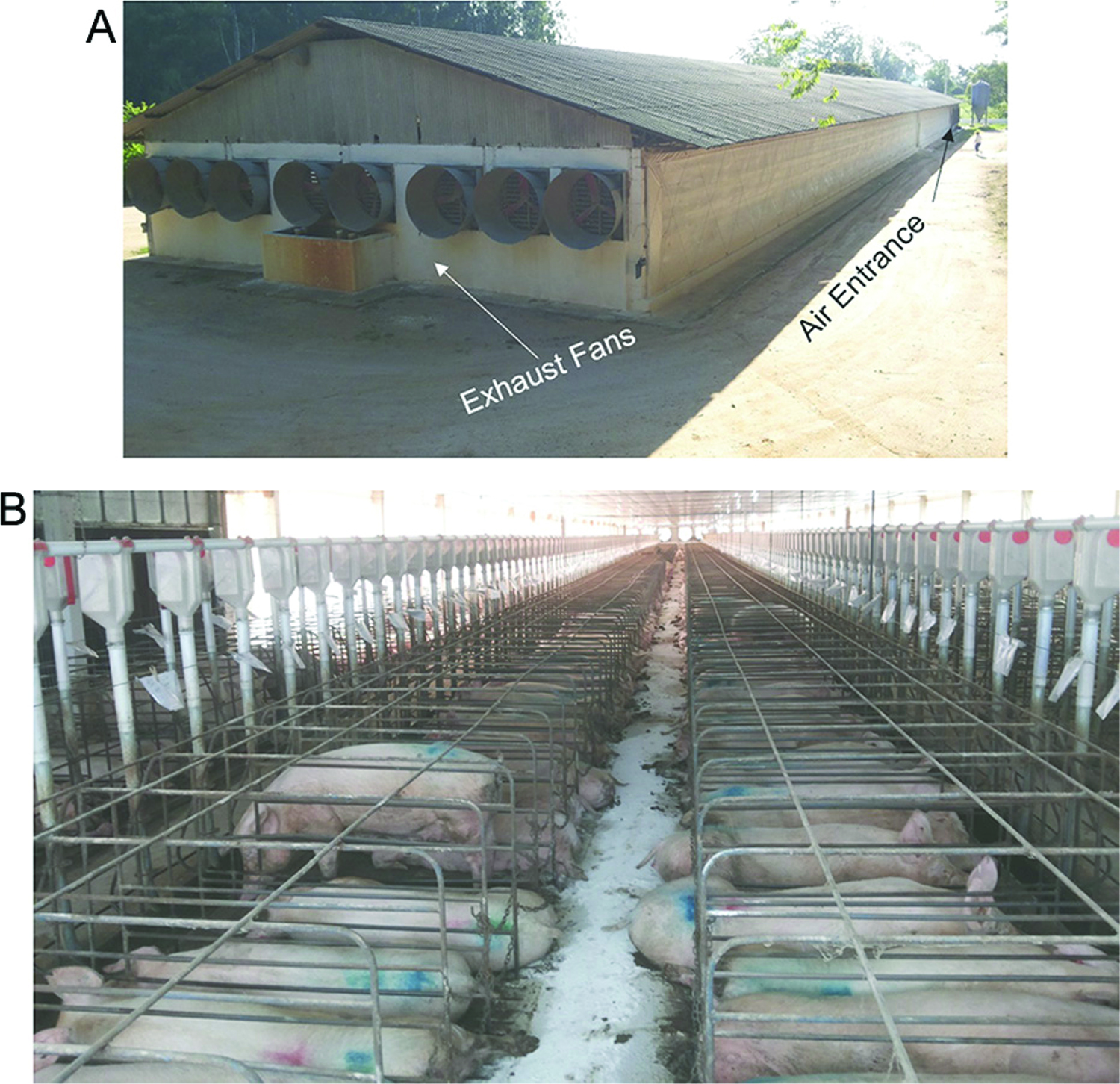
The experimental data were collected in a commercial swine facility located in Itu, in the state of São Paulo, Brazil (South hemisphere, South latitude 23°05′25″, West longitude 47°13′05″, and altitude of 624 m). The barn is dedicated to pregnant sows and its dimensions are 99.61 m long × 15.5 m wide × 3.07 m high. The roof material is fiber-cement and polyethylene painted in white on the ceiling and the walls.

The geometry of the model is shown in Figures 1A and B. The roof can interfere with the airflow, but the facility has an insulated ceiling and the fluid flows between the floor and the ceiling. Therefore, the temperature boundary condition was set only in the ceiling since there was no contact of the upper part of the ceiling (the area between the ceiling and the roof). The area above the ceiling is not included in the mesh.

Figure 1
Facility where data were collected: (A) exhaust fans and air entrance; (B) internal view.

The ventilation system of the building has eight exhaust fans in the east extremity of the barn and two air inlets. One air entrance is in the southern wall and the other is in the northern wall (opposite side of the barn, see Figure 1A). These entrances were equipped with an evaporative panel made of cellulose, measuring 13.48 × 1.74 m (Figure 2). The model of the exhaust fans is a VA 130 (50″) with a diameter of 1.38 m and a 1.5 CV three phase motor.

Figure 2
Measurements of the barn.

Geometry and mesh

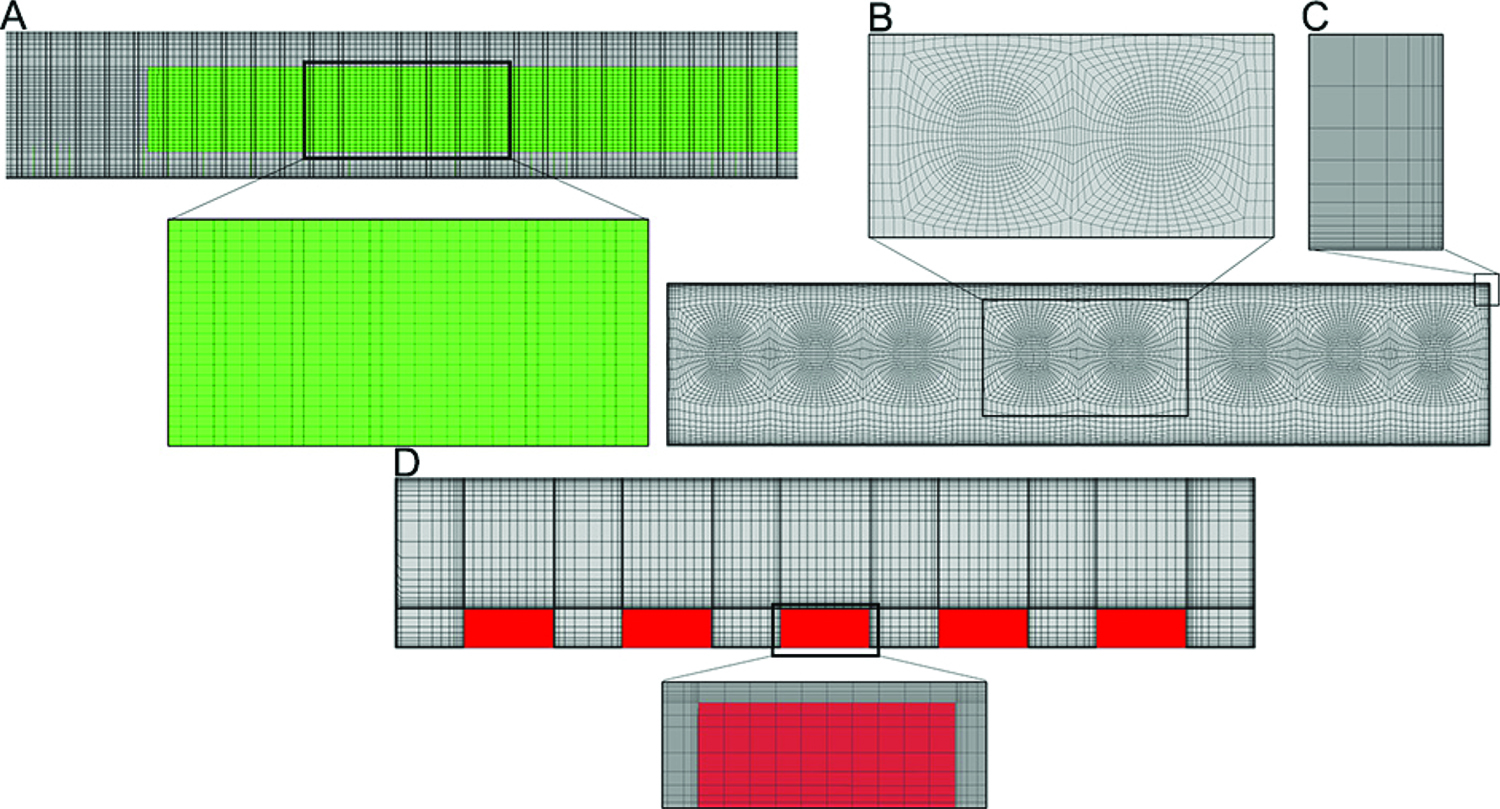
The Ansys Icem 14.0^® software program was used to build the mesh domain. The model was based on the real dimensions of the barn (Figure 2). There were feeders inside the facility, which were not considered in the simulations due to their reduced size compared to the measurements of the barn. Furthermore, they had a negligible influence on the flow. Drinkers were also not considered in the simulation because they were at ground level.

The model domain (barn) was discretized in finite volumes. This mesh was refined in locations with greater fluid flow gradients as air entrance (Figure 3A) and exhaust fans (Figure 3B). There was also mesh refinement near the wall to ensure a sufficient number of nodes to adequately capture the flow change inside the boundary layer (Figure 3C).

Figure 3
Details of the generated mesh: (A) air entrance; (B) exhaust fans; (C) refinement near the wall; (D) volume representing sows.

The sows were housed in cages made of metal bars (Figure 1B). To include these animals in the simulations, it was decided to approximate their shape with boxes (0.7 m high × 0.5 m wide × 1.6 m in length) (Figure 3D). Kwon et al. (2015) also used boxes to represent pigs and the results of their simulations corroborated the experimental data of Zhang and Strom (1999).

Model and governing equations

The equations used for this model are the conservation of mass, momentum and energy (Norton et al., 2007).

Conservation of mass:

(1) $$\frac{{\partial }_{\text{ρ}}}{{\partial }_t}+\frac{\partial }{{\partial }_{x_i}}\left(\text{ρ}{u}_j\right)=0$$

Conservation of momentum:

(2) $$\frac{\partial }{{\partial }_t}\left(\text{ρ}{u}_i\right)+\frac{\partial }{{\partial }_{x_i}}\left(\text{ρ}{u}_i{u}_j\right)=\frac{\partial }{{\partial }_{x_j}}\left[-p{\text{δ}}_{ij}+\text{μ}\left(\frac{\partial u_i}{\partial x_j}+\frac{\partial u_j}{\partial x_j}\right)\right]+\text{ρ}{g}_i$$

Conservation of energy:

(3) $$\frac{\partial }{{\partial }_t}\left(\text{ρ}{C}_{a}T\right)+\frac{\partial }{{\partial }_{x_j}}\left(\text{ρ}{u}_j{C}_{a}T\right)-\left(\frac{\partial }{{\partial }_{x_j}}\text{λ}\frac{\partial T}{\partial x_j}\right)=S_T$$

In the present article, fluid flow was modeled using the k-ε standard turbulence model. This model has been used for CFD modelling on rural constructions (Blanes Vidal et al., 2008; Norton et al., 2009; Wu et al., 2012; Seo and Lee 2013; Zong and Zhang, 2014) due to its favorable convergence behavior and reasonable precision (Launder and Spalding, 1972). The equations of the turbulence model are described as (Equations 4 and 5):

(4) $$\frac{\partial \left(\text{ρ}k\right)}{\partial t}+\frac{\partial \left(\text{ρ}k{u}_i\right)}{\partial x_i}=\frac{\partial }{\partial x_i}\left[\left(\text{μ+}\frac{{\text{μ}}_t}{{\sigma }_k}\right)\frac{\partial k}{\partial x_j}\right]+G_k+G_b-\text{ρε}-Y_M$$

(5) $$\frac{\partial \left(\text{ρε}\right)}{\partial t}+\frac{\partial \left(\text{ρε}{u}_i\right)}{\partial x_i}=\frac{\partial }{\partial x_j}\left[\left(\text{μ+}\frac{{\text{μ}}_t}{{\sigma }_{\text{ε}}}\right)\frac{\partial \text{ε}}{\partial x_j}\right]+C_{1\text{ε}}\frac{\text{ε}}{k}+\left(G_k-C_{3\text{ε}}{G}_b\right)-C_{2\text{ε}}\text{ρ}\frac{{\text{ε}}^2}{k}$$

where k: turbulent kinetic energy (m² s⁻²); μ: viscosity (m² s); μ_t: turbulent viscosity (m² s); σk: turbulent Prandtl number for k (1.0); G_k: generation of turbulent kinetic energy due to the mean velocity variations, (kg m⁻¹ s⁻²); G_b: generation of kinetic energy due to the buoyancy (kg m⁻¹ s⁻²); ε: turbulent dissipation rate (m² s⁻³); Y_M: contribution of the pulsatile expansion associated to the compressible turbulence (kg m⁻¹ s⁻²); σ_ε: turbulent Prandtl number for ε (1.3); C_1ε: constant (1.44); C_2ε: constant (1.92); C_3ε: tanh[u1/u2]; u1: velocity of flow parallel to g_i (gravitational vector); and u2: velocity of flow perpendicular to g_i (gravitational vector).

A number of hypotheses were considered for the development of the model, such as incompressible flow, non-isothermal condition, where the temperature at the surface considered a wall is constant and its value defined as a boundary condition (Table 1), non-slip condition, where the air velocity at surfaces considered walls is zero (parallelograms representing the pigs and all solid surfaces).

Table 1
Boundary Conditions for carrying out the simulation.

Local Surface	Boundary Condition	CFX Condition	Variable	Values
Sow	Wall	No Slip Wall	Temperature	37 °C
Ceiling	Wall	No Slip Wall	Temperature	40 °C
Floor	Wall	No Slip Wall	Temperature	25 °C
West Wall	Wall	No Slip Wall	Temperature	30 °C
East Wall	Wall	No Slip Wall	Temperature	30 °C
North Wall	Wall	No Slip Wall	Temperature	35 °C
South Wall	Wall	No Slip Wall	Temperature	35 °C
			Air Velocity	0.3 m s−1
Air Entrance	Inlet	Normal Speed	Temperature	27.7 °C
Exhaust Fans	Outlet	Pressure	Static Pressure	0 Pa

In order to show how the positioning of the air entrance and exhaust fans influence the temperature profile and air velocity, virtual tests on several different arrangements were carried out. Four CFD simulations are presented, corresponding to four different scenarios (including the one measured in the facility). Each one was characterized according to the different positioning combination of the air entrance and exhaust fans (see Table 2 and Figures 4A, B, C and D).

Table 2
Characteristics of the four different arrangements.

Local	Arrangement	Characteristic
Exhaust Fans	6out_out	Six exhaust fans evenly distributed in the east wall with a distance of 1.03 m between any two pair of exhausts or exhaust and corner of the building. Two exhaust fans were positioned 0.53 m from the corner of the north and south walls.
	8out	Eight exhaust fans positioned at the east wall (distributed as Figure 2).
Air Entrance	2in	two entrances (south and north) (distributed as Figure 2).
	1in	When using one entrance, the area for the airflow is the same as when there are two entrances, totaling in either case 47 m2

Figure 4
Proposed model: (A) 2in_8out, (B) 2in_6out-2out; (C) 1in_8out; (D) 1in_6out-2out.

The air entrance and exhaust fan heights were kept the same in all simulations. This arrangement can be seen in Figure 2.

Data measurement

Data were collected on one day during a typical summer period in Brazil, to generate an average from the data for each locating point, where air temperature (°C) and local air velocity (m s⁻¹) were measured with the use of a hot-wired VelociCalc anemometer. The temperature of the equipment ranged from -18 to 93 °C, with an experimental error of ± 0.1 °C, and air velocity ranged from 0 to 30 m s⁻¹, with a measuring resolution of ± 0.015 m s⁻¹. Air temperature was measured in a 30 point spread in the facility as shown in Figure 5. The anemometers were allocated on a fixed platform, which was moved until the 30 points were measured. The anemometer remained in the same spot for 6 min and an average for the day was obtained afterwards with the temperature being computed for each of the 360 s of the measurement (since the equipment does not record the measurements, the display of the anemometer was filmed during the 6 min and the values recovered afterwards). Similar approaches using the same kind of equipment have been reported in the literature such as in the works of Blanes-Vidal et al., 2008; Kim et al., 2008; Bustamante et al., 2013; Bustamante et al., 2015; and Costa et al., 2014. The height at which the data collection was taken was 0.9 m, slightly higher than the animals’ head height to avoid their damaging the equipment.

Figure 5
Distribution of measuring points throughout the facility.

Two more collections were made near the air entrance beyond points 1 and 30 in order to better define the boundary conditions (air temperature and velocity) (Table 1). following the procedure previously mentioned. Measurements were taken of the air velocity data in only these three places near each air entrance.

A thermal camera was used to obtain the temperature boundary conditions for the wall. Using software for analyzing and reporting, the local values of chosen points of the wall were recovered, which allowed for the estimation of an average value for the temperature. The shorter dimension (the width) of the barn needed two pictures and the longer dimension, five. Within each picture, 50 points were used for estimating the average temperature which was then extended to the 250 points for the longer wall and to 100 points for the shorter wall. The use of thermographic images allows for the conversion of the visible radiation pattern of an object into images that make it possible to see the temperature of any surface (Incropera et al., 2006).

This technique was first developed for military purposes, but it subsequently gained application in several other scientific fields such as aerospace engineering (Avdelidis et al., 2003; Avdelidis and Almond, 2004), agriculture and the food industry (Vadivambal and Jayas, 2011), civil engineering (Khan et al., 2015), and animal science (Case et al., 2012; Cilulko et al., 2013; Brown-Brandl et al., 2013; Soerensen and Pedersen, 2015; Warriss et al., 2006; Lima et al., 2013), amongst others. The temperature measurement, which had previously been taken using thermometers, thermocouples and resistance temperature detectors, is nowadays taken by thermographic equipment (as was the case in this study) and infrared thermometers. Both thermographic image and infrared thermometer (Bustamante et al., 2015; Blanes-Vidal et al., 2008) are non-destructive techniques (Kowalewski et al., 2007). Thermographic images provide a temperature mapping of any surface of interest, while infrared thermometers measure temperature at a specific point.

A value of 0 Pa for the pressure was defined for the pressure boundary condition at the outlet, which is equivalent to 1 atm (Ansys, 2011; Rong et al., 2016; Nam and Han, 2016).

Mesh study

Mesh independence test – Meshes used in CFD models must be sufficiently refined to identify important characteristics of the flow. This refinement is important for correctly estimating variable gradients to guarantee correct flow calculation. Mesh refinement must be carried out in areas of high variable gradients.

The most accurate manner of verifying if a mesh is adequate is to perform a mesh independence test, which consists of analyzing two or more meshes with different refinements, and comparing the results obtained for each mesh. If the result of the two different mesh densities do not vary significantly, the results can be considered mesh independent. Otherwise the mesh needs to be refined and the procedure described above is performed until a mesh independent size is obtained.

It is also necessary to investigate the y⁺ variable (Eq. 6), which varies according to the turbulence model. This parameter represents a dimensionless distance, used to check the location of the first node away from a wall inside the boundary layer. For the standard k-ε turbulence model it should be in the range of 30 < y⁺ < 300 (Andersson et al., 2012). It should also be mentioned that the standard k-ε model always uses the “Scalable Wall Function” approach, built into the software, which assumes that the solid surfaces coincide with the edge of the viscous sublayer, which is the intersection between the linear and the logarithmic near wall velocity profile.

(6) $$y^{+}=\frac{u_{\tau }y}{V}$$

where: u_τ: friction velocity defined as $u=\sqrt{\raisebox{1ex}{${\tau }_w$}\!\left/ \!\raisebox{-1ex}{$\text{ρ}$}\right.}$ used to estimate wall shear stress; ρ is the fluid density at the wall; y: the distance to the nearest wall; and V: the kinematic velocity of the fluid. The dimensionless wall distance (y⁺), usually referred to as yplus in simulation software programs, is the distance from the first mesh node to the wall (Versteeg and Malalasekera, 2007).

Mesh quality – The mesh quality was tested to guarantee the quality. A criterion called “Determinant 3 × 3 × 3” helps to analyze the structured mesh quality. This parameter shows how much the edges of the elements are either distorted or regular. A value of 1 indicates perfectly regular elements and 0 indicates elements with the worst distortion. The values for “Determinant 3 × 3 × 3” above 0.3 indicate a mesh with good quality. The values for the Determinant of the meshes presented in this study were 3 × 3 × 3, all above 0.5.

Model validation – In the present investigation, validation was carried out by comparing the simulated air temperature distribution with data measured in the field (Norton et al., 2013; Seo et al., 2012). The variable compared was the air temperature because the equipment to collect data at multiple locations simultaneously was not available. Preliminary tests have shown the air velocity to vary greatly with time in all of the collection points, and because of this, it was the temperature chosen. To estimate the relative error, the following equation was applied:

(7) $$E=\frac{\left|T_{sim}-T_m\right|}{T_m}*100$$

where: E is the error between the simulated and measured data (%); T_sim = simulated air temperature; T_m = measured air temperature.

Results and Discussion

Mesh independence study and solution monitoring

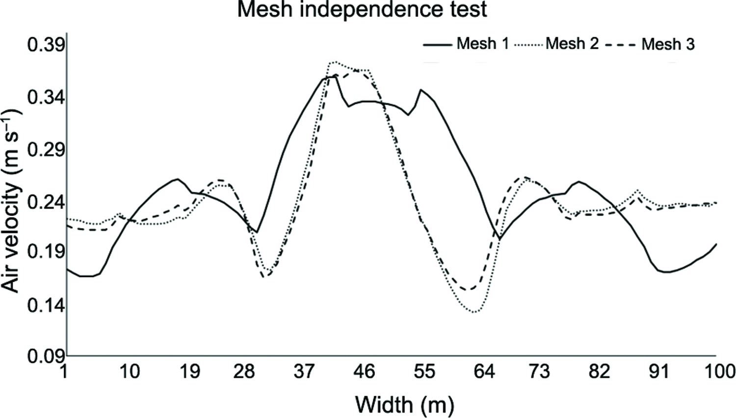
To test mesh independence, the air velocity profile was compared based on a line drawn in the center of the barn where 1000 measuring points had been collected. This line was created between two coordinate points, from a point with coordinates (x = 2 m; y = 0.8 m; z = 50 m) to another point with coordinates (x = 14 m; 0.8 m; z = 50 m) in the interior of the building. It can be observed that the results between the three meshes are very similar, as observed in Figure 6. The mesh densities were: mesh 1 (2,552,572 nodes / 2,346,961 elements), mesh 2 (4,123,408 nodes / 3,884,383 elements) and mesh 3 (4,847,356 nodes / 4,544,989 elements).

Figure 6
Comparison of simulated air velocity between different mesh size elements.

It was observed that mesh 1 showed greater variation compared to mesh 2 and both of these in turn presented little difference to mesh 3. Even between meshes 2 and 3, the greatest variation found was 0.15 m s⁻¹. For this reason, it has been considered that the mesh density of 4,123,408 (mesh 2) elements is sufficiently refined for the simulations.

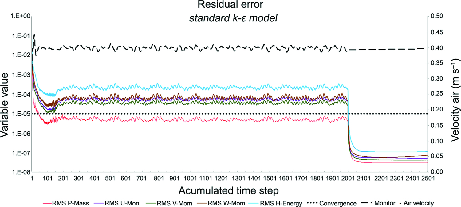
RMS values (Root Mean Square) less than 1 × 10⁻⁵ have been defined as the residual error. The simulations were first carried out in steady state in 2,000 iterations to get a faster convergence. Thereafter, a total time of 25 s with a time step of 0.05 s was simulated resulting in 500 more iterations in order to reduce residual. This was repeated up to 10 times (loops) in an attempt to converge the variable values. In a general manner, all simulations reached the convergence criteria defined in relation to mass, momentum and energy. Furthermore, a monitor was set close to the exhaust, which allowed for observing the value of the air velocity in real time. This is important, since it enables the user to identify when the variable reaches stability and ceases to change in value.

In steady-state, the simulations did not converge after 2,000 iterations (except the RMS of mass). From this result a transient simulation was run and all the variables converged quickly, reaching residue below 10⁻⁷ (Moment and Mass), and 10⁻⁵ (Energy) (Figure 7).

Figure 7
Monitoring of the convergence criteria.

Model validation

The air temperature data measured and simulated were compared by means of the relative error (RE) (Table 3). All the air temperatures measured showed relative errors of less than 5 %, reaching a maximum of around 3 %. These results demonstrate the agreement between simulated and measured air temperatures. In absolute terms, the predicted and measured values presented a maximum discrepancy of 1.02 °C.

Table 3
Difference between simulated and measured temperature and Relative Error.

CP	Sim	Col	Error	CP	Sim	Col	Error
	——— °C ———		%		——— °C ———		%
1	27.7	27.0	2.7	16	31.0	30.9	0.2
2	29.7	29.4	1.0	17	30.6	29.9	2.2
3	30.1	29.9	0.5	18	29.7	29.6	0.5
4	30.7	30.0	2.4	19	28.7	28.2	1.6
5	31.1	30.7	1.4	20	28.4	28.1	0.9
6	31.4	30.4	3.3	21	29.1	28.8	1.1
7	30.8	30.0	2.8	22	28.9	28.5	1.3
8	30.3	29.5	2.8	23	30.4	29.6	2.8
9	29.1	28.3	2.8	24	30.9	30.3	2.0
10	29.1	28.5	2.0	25	31.4	30.7	2.3
11	28.3	27.8	1.9	26	31.2	30.5	2.2
12	28.8	28.3	1.9	27	30.7	30.0	2.5
13	30.6	29.6	3.5	28	30.1	29.2	3.1
14	30.7	30.1	1.9	29	29.7	29.0	2.4
15	31.0	30.1	3.1	30	27.7	28.1	3.0

• Sim = simulated temperature; Col = measured temperature; CP = collection point.

The concordance between the predicted and the actual values collected when observed is clearly shown in Figure 8. These discrepancies are noticed in studies which feature temperature as a validation variable. In the zone occupied by swine there were variations in temperature reported of 1.84 °C above the values measured when the amount of heat generated by the animals was taken from the floor and 0.64 °C below those values collected when the pigs were represented by geometric figures similar to their real forms (Seo et al., 2012) with a relative error of 1 % and 2 % to 0.3 and 4.3 m in height, respectively (Saraz et al., 2013). Norton et al. (2013) investigated a livestock transporter with two decks. They found differences between predicted and measured values from 2 to 4 °C in the top deck which was ventilated mechanically and over 5 °C in the lower deck which was ventilated naturally. This may have been due to a mixture of experimental and numerical errors which cannot be isolated from the data set. The errors may be due partly to the inadequacies of the turbulence modelling or uncertainty related to measuring equipment (Norton et al., 2013). Moreover, a malfunction in the exhaust fans and maintenance problems could be the cause of the errors reported in this investigation.

Figure 8
Comparison between predicted and measured air temperature data at the 30 measuring points at the longitudinal plane.

Overestimated values of the predicted air temperatures can also be viewed in relation to those measured in the field (Figure 8). This probably occurred because the rectangular geometry that represented the animals covers an area larger area than the real ones.

Furthermore, the predicted values without the presence of animals were compared and it was observed that these temperatures were underestimated when compared to the actual data collected. This was expected and was attributed to the absence of a heat source represented by animals in the simulation. Out of the 30 measuring points compared, 21 showed an absolute difference higher than 1.0 °C reaching 3.2 °C.

Proposed model

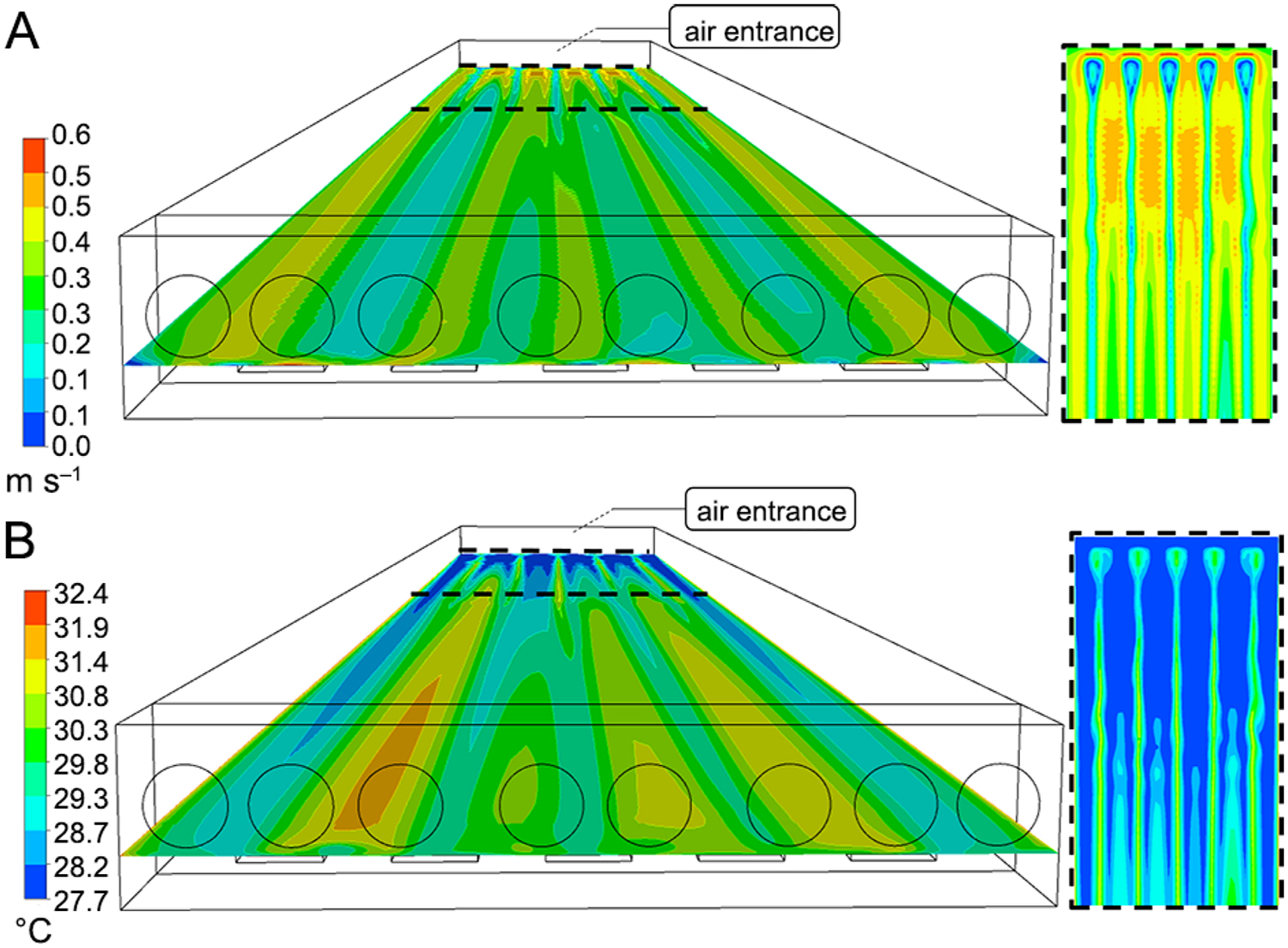
Three scenarios beyond the original case were tested in order to determine whether changes in the positioning of air entrance and exhaust fans can influence the air velocity and temperature. Thus, the following planes were generated: longitudinal plane at a height of 0.9 m and a transversal plane at 20, 50 and 99 m. All the arrangements were compared to the model that represents the previously described field conditions, (Figure 2).

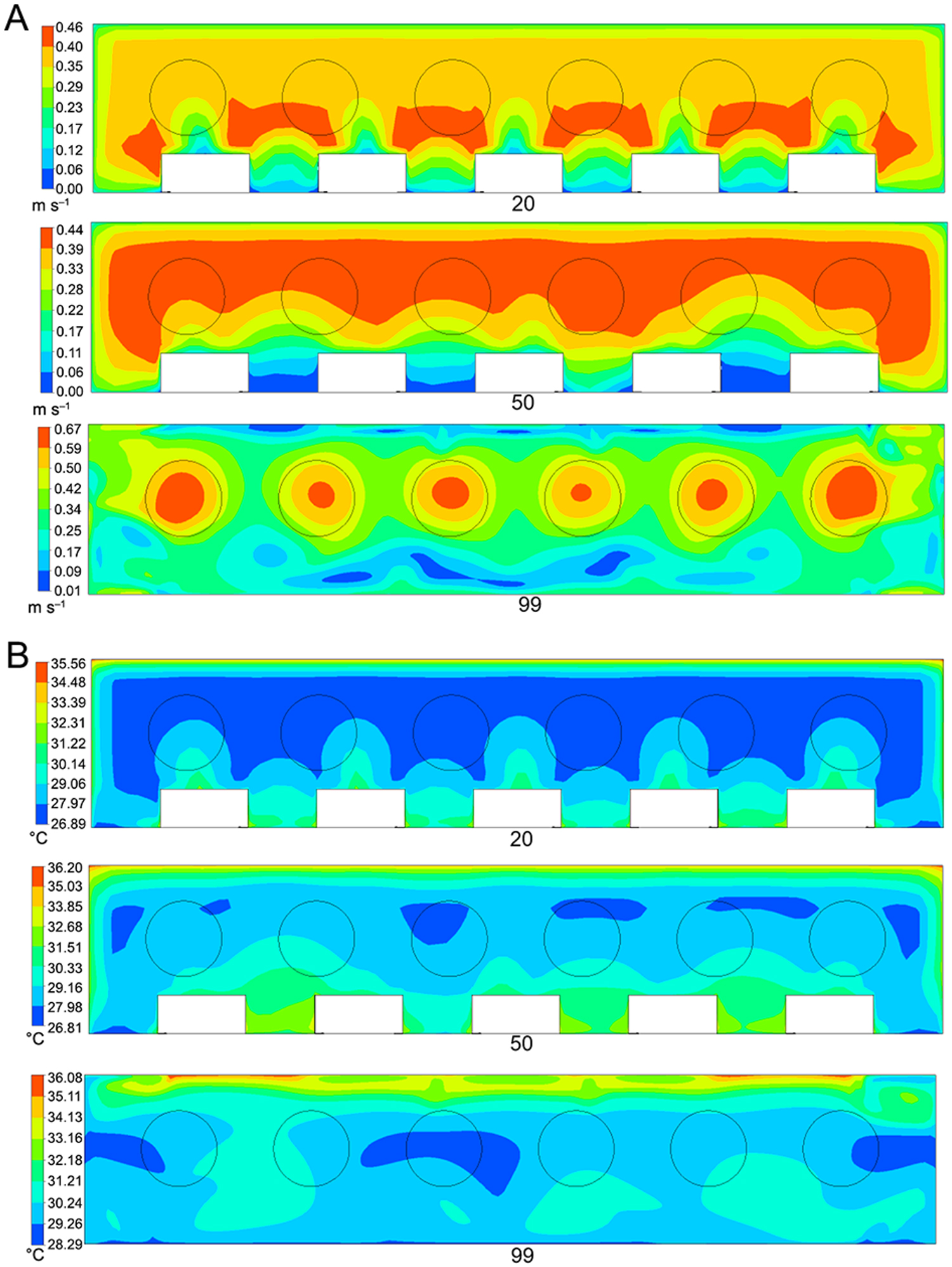
Air velocity showed an increase from the entrance (Figure 9A). A tendency to greater uniformity of the variables was observed as it approached the exhaust fans (Figure 10A and B) and the greatest air velocity was found in the central facility (Figure 9A).

Figure 9
Air velocity (A) and temperature (B) at longitudinal plane at arrangement “2in_8out”.

Another important observation was the “dead zones” (low air velocity at specific points). These places were found near the end of the air inlet at the side walls and at the wall opposite the exhaust fans (Figure 9A). This might be explained by the change in the trajectory of the air when it entered in the north and south sides, being drawn by the exhaust fans toward the east direction. This initial disturbance was not maintained on reaching the exhaust fans.

The simulation model showed that animals housed in the regions of low airflow would be exposed to uncomfortable conditions in situations of high temperatures because the wind is responsible for the loss of heat by convection.

When the original arrangement was simulated (2in_8out), the temperature increased in line with the increasing minimum temperatures (Figure 9B) and were more uniform (Figure 10B) away from the air entrance.

Figure 10
Simulated air velocity (A) and temperature (B) contours in a transversal plane at 20 m, 20 m and 99 m (2in_8out).

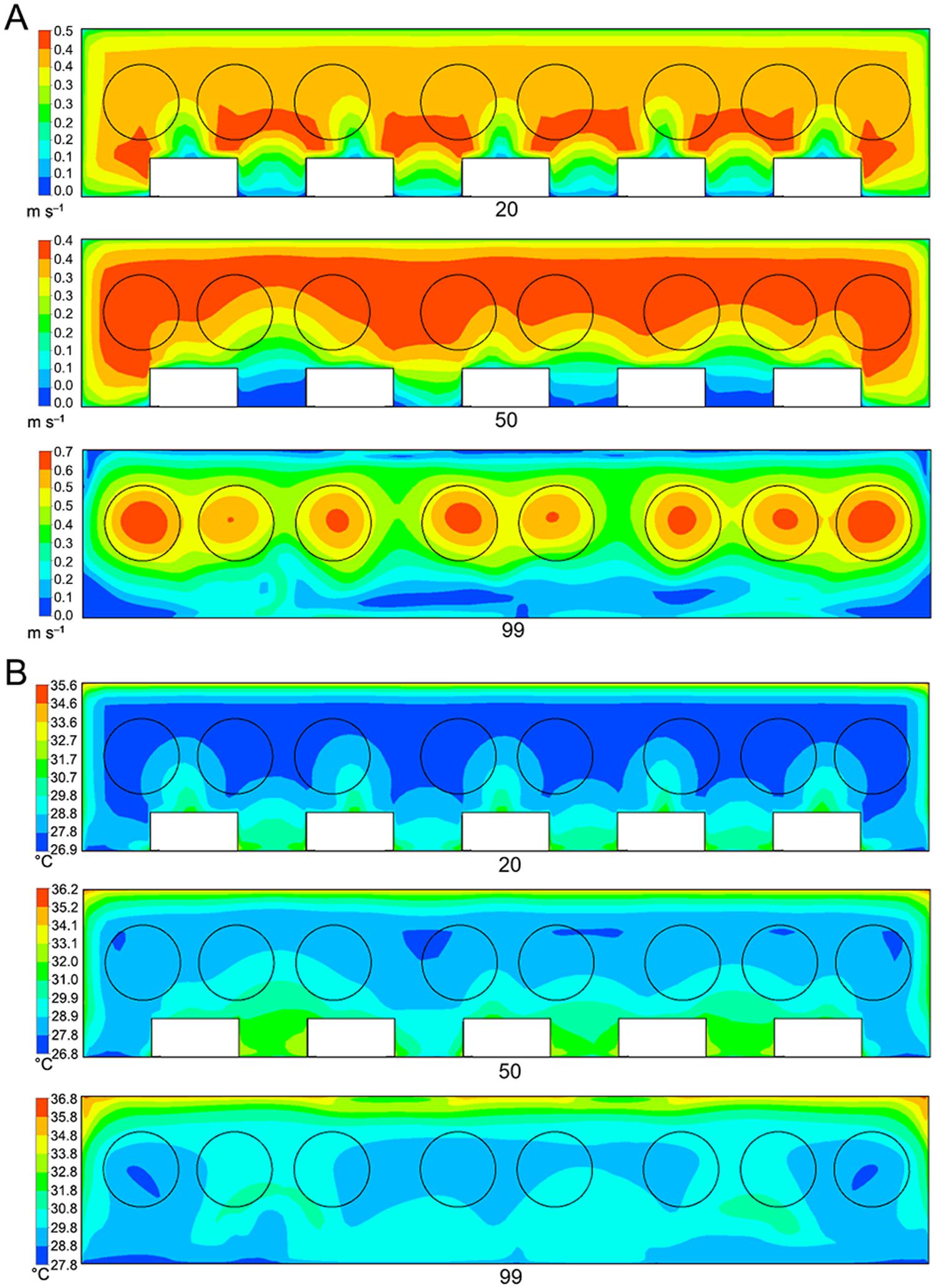
The next arrangement (2in_6out-2out) to be displayed had two exhaust fans in a position that was relative to the original configuration (Figures 11A and B to Figures 12A and B). The two scenarios showed similarity in the distribution pattern in terms of temperature and air velocity. Thus, the simulations showed that relocating the exhaust fans would not have influenced the pattern of variables.

Figure 11
Air velocity (A) and temperature (B) at longitudinal plane with arrangement “2in_6out-2out”.

Figure 12
Simulated air velocity (A) and temperature (B) contours in a transversal plane at 20 m, 20 m and 99 m (2in_6out-2out).

It was observed that the “dead zones” where the air velocity was zero, no longer exist when the air intake was changed to the west wall and the exhaust fans were kept in the same position (1in_6out-2in) (Figure 13A and B). It was possible to see five lines coinciding with the sow positions. The volumes in these lines represent sows and they were considered physical barriers, being responsible for a reduction in air velocity beyond the air entrance. The variables had the same pattern along the transverse sections (Figure 14A and B) which is important to attempts to provide the same conditions for all the animals housed in the facility.

Figure 13
Air velocity (A) and temperature (B) at longitudinal plane at arrangement “1in_6out-2out”.

Figure 14
Simulated air velocity (A) and temperature (B) contours in a transversal plane at 20 m, 20 m and 99 m (1in_6out-2out).

By keeping a single incoming air current combining eight exhaust fans (1in_8out), the same distribution pattern of temperature and air velocity was observed (Figures 15A and B and Figures 16A and B), as had been previously seen in the arrangement 1in_6out-2out.

Figure 15
Air velocity (A) and temperature (B) at longitudinal plane at arrangement “1in_8out”.

Figure 16
Simulated air velocity (A) and temperature (B) contours in a transversal plane at 20 m, 20 m and 99 m (1in_8out).

Average values of air velocity and temperature were compared in the exhaust fans (Table 4). Generally, average temperatures and air velocities observed in exhaust fans were similar across all the arrangements tested. Moreover, positioning the air entrances had greater influence than exhaust fans on the distribution of variables within the facility. The eight exhaust fans were set to air outlets in CFX Post. i.e., all of them were working at the time of the simulation. Thus, this work does not attempt to assess the comfort zone of the animals, but rather the effectiveness of the CFD technique in predicting environmental phenomena in animal facilities influenced by air entrance and exhaust fans positioning.

Table 4
Influence of arrangement on air velocity average at the exhaust fans.

Arrangement	Air velocity	Air temperature
	m s−1	°C
2in_8out	1.3	30.8
2in_6out-2out	1.4	30.3
1in_8out	1.4	30.2
1in_6out-2out	1.4	30.2

Conclusion

CFD is a promising tool for the environmental study of animal facilities since it makes it possible to visualize the phenomena in terms of airflow direction and temperature distribution.

The simulations were validated using temperature data. Animal presence in the domain has been shown to have importance, because their absence results in an overestimation of the temperature values and increases the differences between the simulated and experimental data.

The simulated models in most sections had a uniform distribution of airflow and temperature, but there was an occurrence of poor air circulation and higher temperatures immediately next to the air entrances. The simulations showed that the position of the air entrances exerted a greater influence on temperature distribution.

The proposed models do not present differences in average temperature at the outlets, but on the other hand, the arrangements with only one air entrance (1in_8out and 1in_6out-2out) did not demonstrate dead zones near the air intakes. Therefore, improving a facility with mechanical ventilation is a viable proposition for avoiding or minimizing these regions.

Acknowledgements

The authors are grateful to the CNPq (Brazilian National Council for Scientific and Technological Development) for the scholarship granted to the first author (Doctor Degree).

References

• ANSYS. 2011. ANSYS CFX: Solver Theory Guide: 14.0. Ansys, Canonsburg, PA, USA.
• Avdelidis, N.P.; Almond, D.P. 2004. Transient thermography as a through-skin imaging technique for aircraft assembly. Insight-Non-Destructive Testing and Condition Monitoring 46: 200-202.
• Avdelidis, N.P.; Hawtin, B.C.; Almond, D.P. 2003. Transient thermography in the assessment of defects of aircraft composites. NDT & E International 36: 433-439.
• Andersson, B.; Andersson, R.; Håkansson, L.; Mortensen, M.; Sudiyo, R.; van, W.; van Wachem, B. 2012. Computational Fluid Dynamics for Engineers. Cambridge University Press, Cambridge, UK.
• Bartzanas, T.; Kittas, C.; Sapounas, A.A.; Nikita-Martzopoulou, C.H. 2007. Analysis of airflow through experimental rural buildings: sensitivity to turbulence models. Biosystems Engineering 97: 229-239.
• Blanes-Vidal, V.G.E.; Balasch, S.; Torres, A.G. 2008. Application of computational fluid dynamics to the prediction of airflow in a mechanically ventilated commercial poultry building. Biosystems Engineering 100: 105-116.
• Bloemhof, S.; Mathur, P.K.; Knol, E.F.; van der Waaij, E.H. 2013. Effect of daily environmental temperature on farrowing rate and total born in dam line sows. Journal of Animal Science 91: 2667-2679.
• Bustamante, E.; García-Diego, F.; Calvet, S.; Estélles, F.; Béltran, P.; Hospitaller, A.; Torres, A.G. 2013. Exploring ventilation efficiency in poultry buildings: the validation of computational fluid dynamics (CFD) in a cross-mechanically ventilated broiler farm. Energies 6: 2605-2623.
• Bustamante, E.; García-Diego, F.-J.; Calvet, S.; Torres, A.G.; Hospitaler, A. 2015. Measurement and numerical simulation of air velocity in a tunnel-ventilated broiler house. Sustainability 7: 2066-2085.
• Brown-Brandl, T.M.; Eigenberg, R.A.; Purswell, J.L. 2013. Using thermal imaging as a method of investigating thermal thresholds in finishing pigs. Biosystems Engineering 114: 327-333.
• Case, L.A.; Wood, B.J.; Miller, S.P. 2012. Investigation of body surface temperature measured with infrared imaging and its correlation with feed efficiency in the turkey (Meleagris gallopavo). Journal of Thermal Biology 37: 397-401.
• Cilulko, J.; Paweł, J.; Bogdaszewski, P.; Szczygielska, E. 2013. Infrared thermal imaging in studies of wild animals. European Journal of Wildlife Research 59: 17-23.
• Costa, A.; Ismayilova, G.; Borgonovo, F.; Viazzi, S.; Berckmans, D.; Guarino, M. 2014. Image-processing technique to measure pig activity in response to climatic variation in a pig barn. Animal Production Science 54: 1075-1083.
• Incropera, F.P.; Dewitt, D.P.; Bergman, T.L.; Lavine, A.S. 2006. Fundamentals of Heat and Mass Transfer. John Wiley, New York, NY, USA.
• Khan, F.; Bolhassani, M.; Kontsos, A.; Hamid, A.; Bartoli, I. 2015. Modeling and experimental implementation of infrared thermography on concrete masonry structures. Infrared Physics & Technology 69: 228-237.
• Kim, K.Y.; Ko, H.J.; Kim, H.T.; Kim, Y.S.; Roh, Y.M.; Lee, C.M.; Kim, C.N. 2008. Quantification of ammonia and hydrogen sulfide emitted from pig buildings in Korea. Journal of Environmental Management 88: 195-202.
• Kowalewski, T.; Ligrani, P.; Dreizler, A.; Schulz, C.; Fey, U.; Egami, Y. 2007. Temperature and heat flux. p. 487-561. In: Tropea, C.; Yarin, A.; Foss, J.F., eds. Springer handbook of experimental fluid mechanics. Springer, Heidelberg, Germany.
• Kwon, K-S.; Lee, I-B.; Zhang, G.Q.; Ha, T. 2015. Computational fluid dynamics analysis of the thermal distribution of animal occupied zones using the jet-drop-distance concept in a mechanically ventilated broiler house. Biosystems Engineering 136: 51-68.
• Launder, B.E.; Spalding, D.B. 1972. Lectures in Mathematical Models of Turbulence. Academic Press, London, UK.
• Lima, V.; Piles, M.; Rafel, O.; López-Béjar, M.; Ramón, J.; Velarde, A.; Dalmau, A. 2013. Use of infrared thermography to assess the influence of high environmental temperature on rabbits. Research in Veterinary Science 95: 802-810.
• Liu, B.; Zeng, H.; Lin, Y.; Liu, S.; Zheng, H.; You, C.; Shi, H.; Lan, J.; LI, Z.; Tang, J.; Huang, Q. 2015. Design of environmental monitoring and control system for large-scale pig house with fermentation bed. Agricultural Science & Technology 16: 391-399.
• Nam, S.-H.; Han, H. 2016. Computational modeling and experimental validation of heat recovery ventilator under partially wet conditions. Applied Thermal Engineering 95: 229-235.
• Noblet, J.; Dourmad, J.Y.; Le Dividich, J.; Dubois, S. 1989. Effect of ambient temperature and addition of straw or alfalfa in the diet on energy metabolism in pregnant sows. Livestock Production Science 21: 309-324
• Norton, T.; Grant, J.; Fallon, R.; Sun, D-W. 2009. Assessing the ventilation effectiveness of naturally ventilated livestock buildings under wind dominated conditions using computational fluid dynamics. Biosystems Engineering 103: 78-99.
• Norton, T.; Sun, D.; Grant, J.; Fallon, R.; Dodd, V. 2007. Applications of computational fluid dynamics (CFD) in the modelling and design of ventilation systems in the agricultural industry: a review. Bioresource Technology 98: 2386-2414.
• Norton, T.; Kettlewell, P.; Mitchell, M. 2013. A computational analysis of a fully-stocked dual-mode ventilated livestock vehicle during ferry transportation. Computers and Electronics in Agriculture 93: 217-228.
• Rong, L.; Nielsen, P.V.; Bjerg, B.; Zhang, G. 2016. Summary of best guidelines and validation of CFD modeling in livestock buildings to ensure prediction quality. Computers and Electronics in Agriculture 121: 180-190.
• Saraz, J.A.O.; Martins, M.A.; Rocha, K.S.O.; Machado, N.S.; Velasques, H.J.C. 2013. Use of computational fluid dynamics to simulate temperature distribution in broiler houses with negative and positive tunnel type ventilation systems. Revista U.D.C.A. Actualidad & Divulgación Científica 16: 159-166.
• Seo, I-H.; Lee, I.; Moon, O.; Kimc, H.; Hwanga, H.; Hong, S.; Bitoga, J.P.; Yoo, J.; Kwon, K.; Kima, Y.; Han, J. 2009. Improvement of the ventilation system of a naturally ventilated broiler house in the cold season using computational simulations. Biosystems Engineering 104: 106-117.
• Seo, I.; Lee, I. 2013. CFD Application for estimation of airborne spread of HPAI (Highly Pathogenic Avian Influenza). Acta Horticulturae 1008: 57-62.
• Seo, I.; Lee, I.; Moon, O.; Honga, S.; Hwanga, H.; Bitog, J.P.; Kwona, K.; Yec, Z.; Lee, J. 2012. Modelling of internal environmental conditions in a full-scale commercial pig house containing animals. Biosystems Engineering 111: 91-106.
• Soerensen, D.D.; Pedersen, L.J. 2015. Infrared skin temperature measurements for monitoring health in pigs: a review. Acta Veterinaria Scandinavica 57: 5.
• Van Rensburg, L.J.; Spencer, B.T. 2014. The influence of environmental temperatures on farrowing rates and litter sizes in South African pig breeding units. Onderstepoort Journal of Veterinary Research 81: 1-7.
• Vadivambal, R.; Jayas, D.S. 2011. Applications of thermal imaging in agriculture and food industry: a review. Food and Bioprocess Technology 4: 186-199.
• Versteeg, H.K.; Malalasekera, W. 2007. An Introduction to Computational Fluid Dynamics. 2ed. Pearson Education, London, UK.
• Warriss, P.D.; Pope, S.J.; Brown, S.N.; Wilkins, L.J.; Knowles, T.G. 2006. Estimating the body temperature of groups of pigs by thermal imaging. Veterinary Record 158: 331-334.
• Wu, W.; Zhai, J.; Zhang, G.; Nielsen, P.V. 2012. Evaluation of methods for determining air exchange rate in a naturally ventilated dairy cattle building with large openings using computational fluid dynamics (CFD). Atmospheric Environment 63: 179-188.
• Zhang, G.; Strom, J.S. 1999. Jet drop models for control of non-isothermal free jets in a side-wall multi-inlet ventilation system. Transactions of the ASAE 42: 1121-1126.
• Zong, C.; Zhang, G. 2014. Numerical modelling of airflow and gas dispersion in the pit headspace via slatted floor: comparison of two modelling approaches. Computers and Electronics in Agriculture 109: 200-211.

Edited by

Edited by: Dionysis Bochtis/Paulo Cesar Sentelhas

Publication Dates

• Publication in this collection
  May-Jun 2018

History

• Received
  14 Mar 2016
• Accepted
  14 Feb 2017