Rheological behavior of marine soil in submarine debris flows subjected to low temperatures

Abstract

Deep-water regions, such as the Brazilian Pre-salt, are characterized by decreasing temperatures with increasing depth, which causes changes in the rheological parameters of marine soils, which is essential in the context of submarine debris flows. To investigate these effects, rheological characterization was performed through tests conducted at 6°C, 13°C, and 20°C, using a concentric cylinder rheometer programmed to apply a shear rate ranging from 0 to 100 s^-1. The flow curves obtained were analyzed using the Bilinear rheological model, which describes the behavior of the soil before and after the yield stress, defined as Regimes I and II, respectively. As the temperature decreased, the results revealed a significant increase in yield stress, indicating that marine soils exhibit greater shear strength at lower temperatures. Additionally, correlation curves were plotted for the yield stress as a function of the liquidity index using the model proposed by Hotta et al. (2024) for different temperatures and three different correlation equations were obtained, one for each temperature. The analysis showed that the yield stress decreased exponentially with increasing liquidity index and that higher water content reduced the influence of temperature on the rheological behavior of the soil. Based on these findings, a rheological model was developed that incorporates variations in the liquidity index and temperature, enabling a more accurate prediction of yield stress as a function of these two variables These findings are highly valuable for understanding the behavior of soils during submarine debris flows, as the material behaves like a fluid and its movement is governed by rheological properties.

Keywords:
Soil rheology; Marine soil; Submarine debris flow; Temperature

1. Introduction

Submarine mass movements are associated with various disasters, such as the collapse of offshore platforms, failures in engineering installations, damage to pipelines and cable systems, resulting in oil and gas leaks, interruptions in energy supply and environmental pollution. They are also cited as potential causes of devastating tsunamis, with fatal consequences (Fan et al., 2022; Locat & Lee, 2002; Schambach et al., 2020; Wang et al., 2024).

The triggering mechanisms for submarine mass movements are complex and numerous, including earthquakes, faults, rapid sedimentation, gas hydrates, waves, tsunamis, human activity, erosion processes, volcanism, salt diapirism, flooding events, and others (Guo et al., 2020; Kaminski et al., 2021; Liu et al., 2020b; Masson et al., 2006; Nian et al., 2019; Urgeles & Camerlenghi, 2013).

In this context, submarine debris flows represent one of the greatest offshore geological risks and accurate prediction of their impact has become an essential element in offshore engineering projects (Nian et al., 2018). The peculiarity of these events lies in the fact that they are analyzed as non-Newtonian fluids (Tsugawa et al., 2019).

Submarine debris flow modeling is based on rheological models, which accurately describe the shear stress versus shear rate behavior (Rui & Yin, 2019). Therefore, studying the rheological parameters of marine soil is essential for understanding and predicting its behavior under flow conditions, taking into account the hydrodynamic factors that influence its dynamics.

Although the literature presents several rheological studies involving soils with varying water contents (Jeong, 2014; Liu et al., 2020a; Messaoudi et al., 2018; Nie et al., 2020; Shakeel et al., 2022), a significant gap remains in understanding the behavior of marine soils under the influence of low temperatures (Meng et al., 2018), which can significantly alter the rheological properties of these soils.

This article aims to investigate the rheological behavior of marine soils in submarine debris flows, considering the impact of water incorporation and the influence of low temperatures. Laboratory tests were conducted using a rheometer, with samples prepared at controlled water content and temperature, covering Liquidity Index (LI) values between 1.1 and 2.0, temperatures from 6°C to 20°C, and shear rates ranging from 0 to 100 s^-1. Compared with previous studies, this work stands out by analyzing the experimental data using a Bilinear rheological model whose yield stress parameter has been shown to be equivalent to the undrained shear strength obtained with the rheometer. In practical terms, this equivalence provides a clear physical significance to the rheological yield stress and enables a more consistent interpretation of the marine soil behavior under submarine flow conditions. Additionally, assessing the influence of temperature is essential, as submarine flows can occur at different depths where thermal gradients may significantly affect the rheological response of marine soils.

2. Soil and temperature in submarine debris flows

2.1 Submarine debris flow

The behavior of submarine debris flows can be understood through four distinct stages (Hotta et al., 2024): 1) failure, initiated by a triggering mechanism; 2) flow formation, where the soil mixes with water, exhibiting non-Newtonian fluid characteristics; 3) debris flow development; 4) deposition, where the material accumulates on the seabed.

In this context, soil properties change continuously, and to investigate this behavior in detail, it is essential to consider the hydrodynamic effects involved in this process. Therefore, a comprehensive understanding of this phenomenon encompasses both soil mechanics and fluid mechanics (Mosher et al., 2010), which complement each other and can be studied using the principles of fluid rheology.

The most important rheological parameters are viscosity ($\mu$) and yield stress (${\tau }_0$) (Barnes et al., 2005). Newton’s law of viscosity describes the ability of a fluid material to resist shear-induced flow. The yield stress in rheology represents the onset of the flow (Locat & Lee, 2009). According to Mothe (2006), the viscosity of a material can depend on six independent parameters: physicochemical nature, temperature, pressure, shear rate, time and electric field.

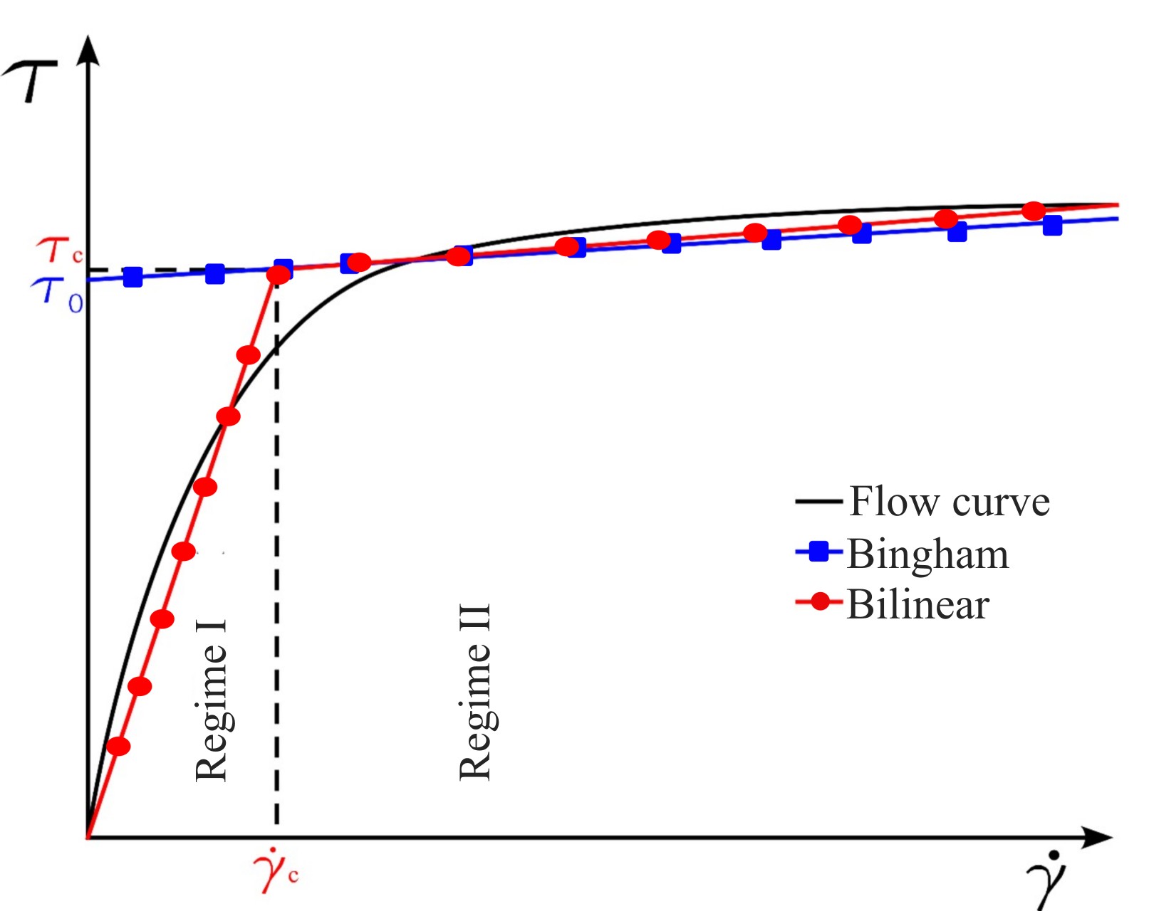
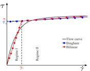
Soil behavior is studied using rheological models, with the Herschel-Bulkley, Bingham, and Bilinear models being the most commonly applied in the context of submarine debris flows (Barnes et al., 2005). Different to the Heschel-Bulkley model, the Bingham and Bilinear models have a yield stress (${\tau }_0)$ with physical significance, as this parameter can be correlated with the undrained shear strength of the soil obtained through rheometer testing (Hotta et al., 2024; Lima et al., 2024). The Bilinear Model differs from the Bingham model in that it accounts for the section of the flow curve - shear rate ($\dot{\gamma }$) x shear stress ($\tau$) - that precedes the critical shear stress (${\tau }_c$) and its corresponding shear rate (${\dot{\gamma }}_c$). This section is referred to as regime I, while the subsequent part is Regime II, as described in Equations 1 and 2 and shown in Figure 1.

Figure 1
Flow curve example, Bingham Model, Bilinear model - regime I and II (Hotta et al., 2024).

$\text{Regime I}(\dot{\gamma }<{\dot{\gamma }}_c)\to \tau ={\mu }_1.\dot{\gamma }$ (1)

$\text{Regime II}\left(\dot{\gamma }>{\dot{\gamma }}_c\right)\to \tau ={\tau }_0+{\mu }_2.\dot{\gamma }$ (2)

Hotta et al. (2024) proposed a rheological model to describe the behavior of marine soils, incorporating the yield stress based on the Bilinear model and accounting for the influence of water content through the liquidity index. This model is particularly relevant for studying submarine debris flows - because the properties of the soil change continuously with water incorporation. However, this model does not account for variations in soil temperature, as the tests were conducted with soil at 24°C.

2.2 Temperature in the offshore environment

The exploration of offshore resources in the Brazilian Pre-salt occurs at depths of more than 1,000 meters, where seawater temperatures are significantly low. Leffler et al. (2011) reported typical values ranging from 30 to 35°F (-1.1 to 1.7°C). Morais (2013) notes that, in Marlim Field, temperatures reach approximately 4°C at this and that such low-temperature conditions pose considerable challenges for oil exploration, particularly with regard to the behavior of marine soils.

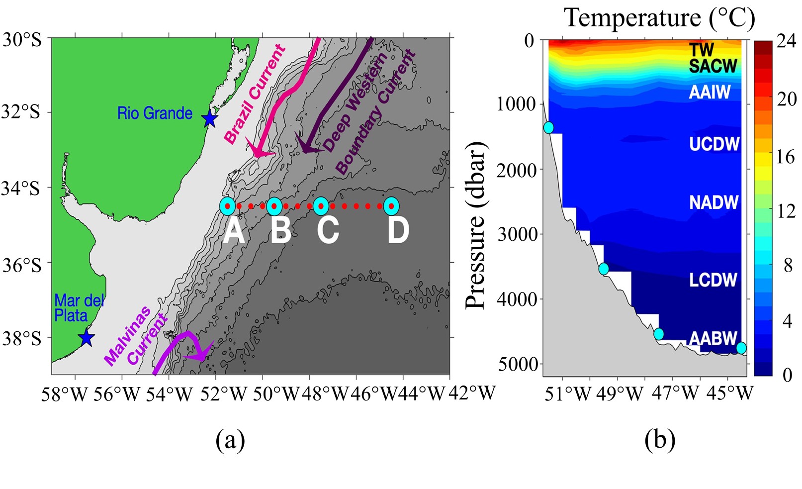
Meinen et al. (2020) presented temperature measurements at four points in the Argentine Basin (Figure 2), using a monitoring system capable of recording thermal data up to depths of exceeding 4,000 meters. The depths of the main water layers were identified using the following acronyms: TW = Tropical Water; SACW = South Atlantic Central Water; AAIW = Antarctic Intermediate Water; UCDW = Upper Circumpolar Deep Water; NADW = North Atlantic Deep Water; LCDW = Lower Circumpolar Deep Water; AABW = Antarctic Bottom Water. The results showed temperatures close to 0°C at the depths of LCDW and AABW, highlighting the extreme conditions of the deep-sea environment.

Figure 2
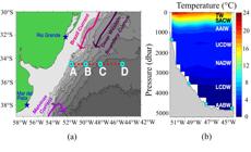
Argentine Basin: (a) Map showing the locations of the temperature profiles collected. The bathymetric of the data set is shown with contours filled in gray with a contour interval of 500m. Schematic arrows indicate the locations of the main ocean currents nearby; (b) Vertical temperature section averaged over four sections (Meinen et al., 2020).

When studying submarine debris flow, it is essential to consider the impact of temperature on the seabed environment. At lower temperatures, the reduction in Brownian motion - random movement of microscopic particles in suspension, caused by collisions with fluid molecules – (Halliday, 2022) contributes to a more stable and structured particle arrangement, leading to greater soil strength. This effect is reflected in the increase in rheological parameters, such as the yield stress and viscosity (Guo et al., 2020). Nian et al. (2018), based on rheological tests using the Herschel-Bulkley model, observed that average shear stress and viscosity of seabed flows at 0.5°C were up to 36.3% higher than those tested at 22°C (room temperature). These results indicate that low temperatures significantly influence the rheological properties of debris flows, representing a key factor in their mobility and overall behavior.

3. Materials and methods

3.1 Soils tested

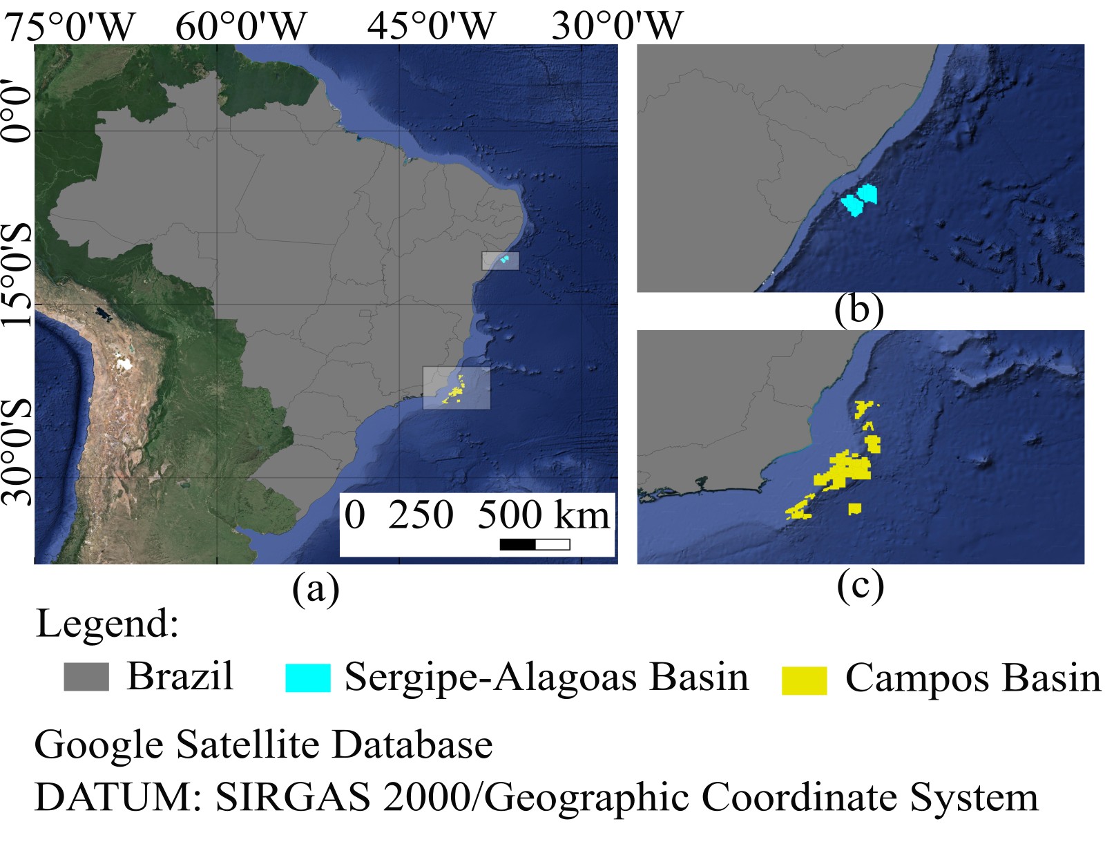
The seabed samples were collected from two Brazilian offshore continental platforms located in the Campos Basin (RJ) and the Sergipe-Alagoas Basin (SE/AL), as illustrated in Figure 3. The geological characteristics and geomorphology of the region have been extensively discussed by Carneiro et al. (2017) and Figueiredo et al. (2015), respectively.

Figure 3
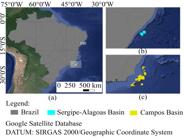
Sample location maps, highlighting: (a) Brazil; (b) Sergipe-Alagoas Basin; (c) Campos Basin.

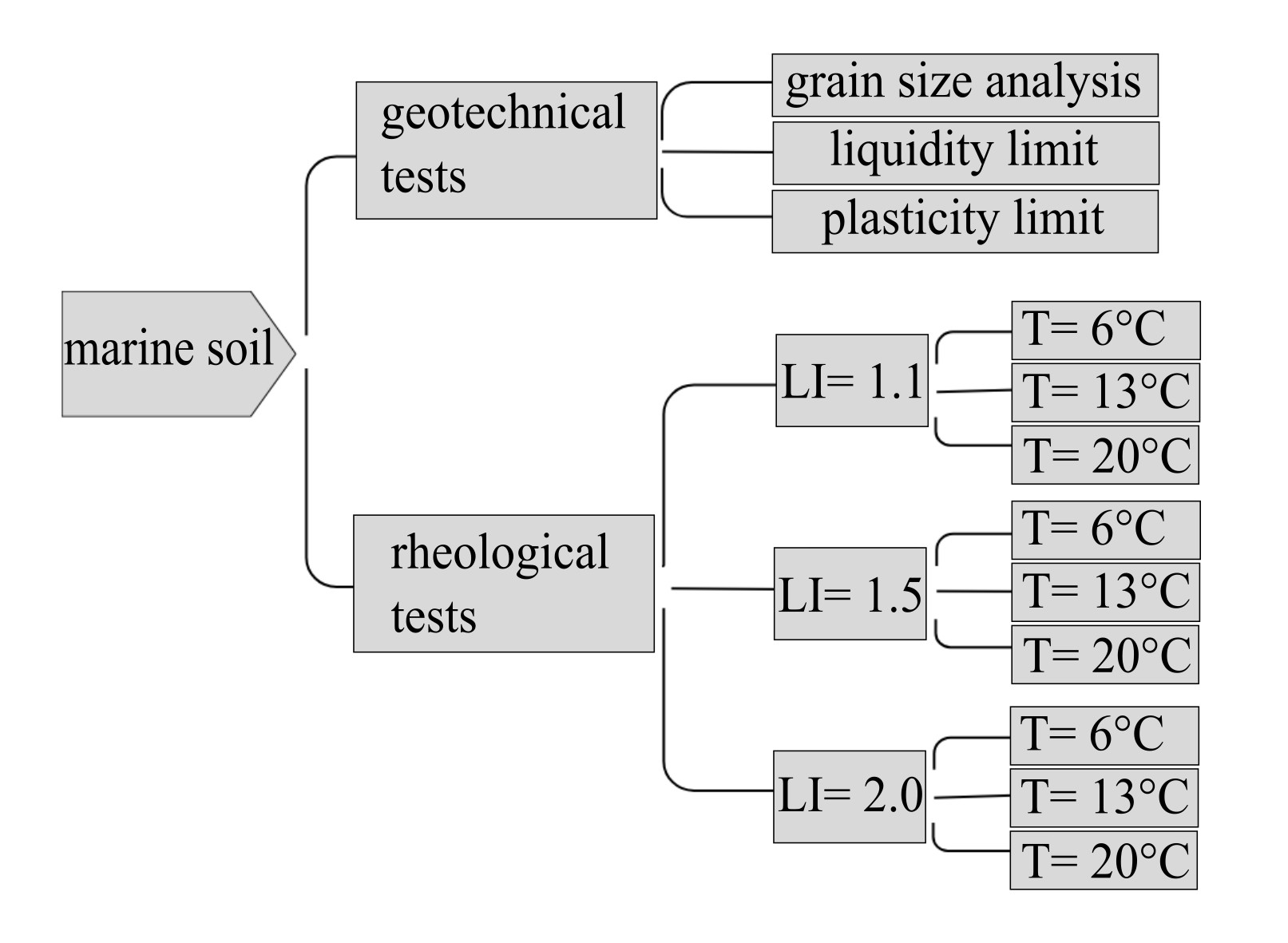
Ten representative samples were analyzed in laboratory tests: five from the Sergipe-Alagoas Basin (SE/AL) and five from the Campos Basin (RJ). Obtained from depths between 20 and 60 meters below the seafloor, these samples consist of in situ marine sediments from the actual depositional environment. The samples were then subjected to geotechnical characterization and rheological tests, as shown in Figure 4.

Figure 4
Characteristics of the tests carried out. Subtitle: LI = Liquidity Index; T = temperature.

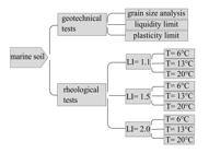
Geotechnical testing of the particle size, plasticity limit ($w_P)$ and liquidity limit ($w_L$) tests were carried out in accordance with international standards: ASTM D6913 (ASTM, 2021), ASTM D7928 (ASTM, 2017) and ASTM D4318 (ASTM, 2018).

3.2 Sample preparation

For the execution of the tests, the soil must have a water content sufficiently high to exceed its liquid limit ($w_L$), which varies for each sample. To standardize the results, the Liquidity Index ($\text{LI}$), Equation 3, was used as a reference. Thus, distilled water was added to the samples until the water content (𝑤) reached the value corresponding to the desired $\text{LI}$ for each test. It is important to note that, in the equation, 𝑤_𝑃 refers to the plastic limit.

$LI=\frac{w-w_P}{w_L-w_P}$ (3)

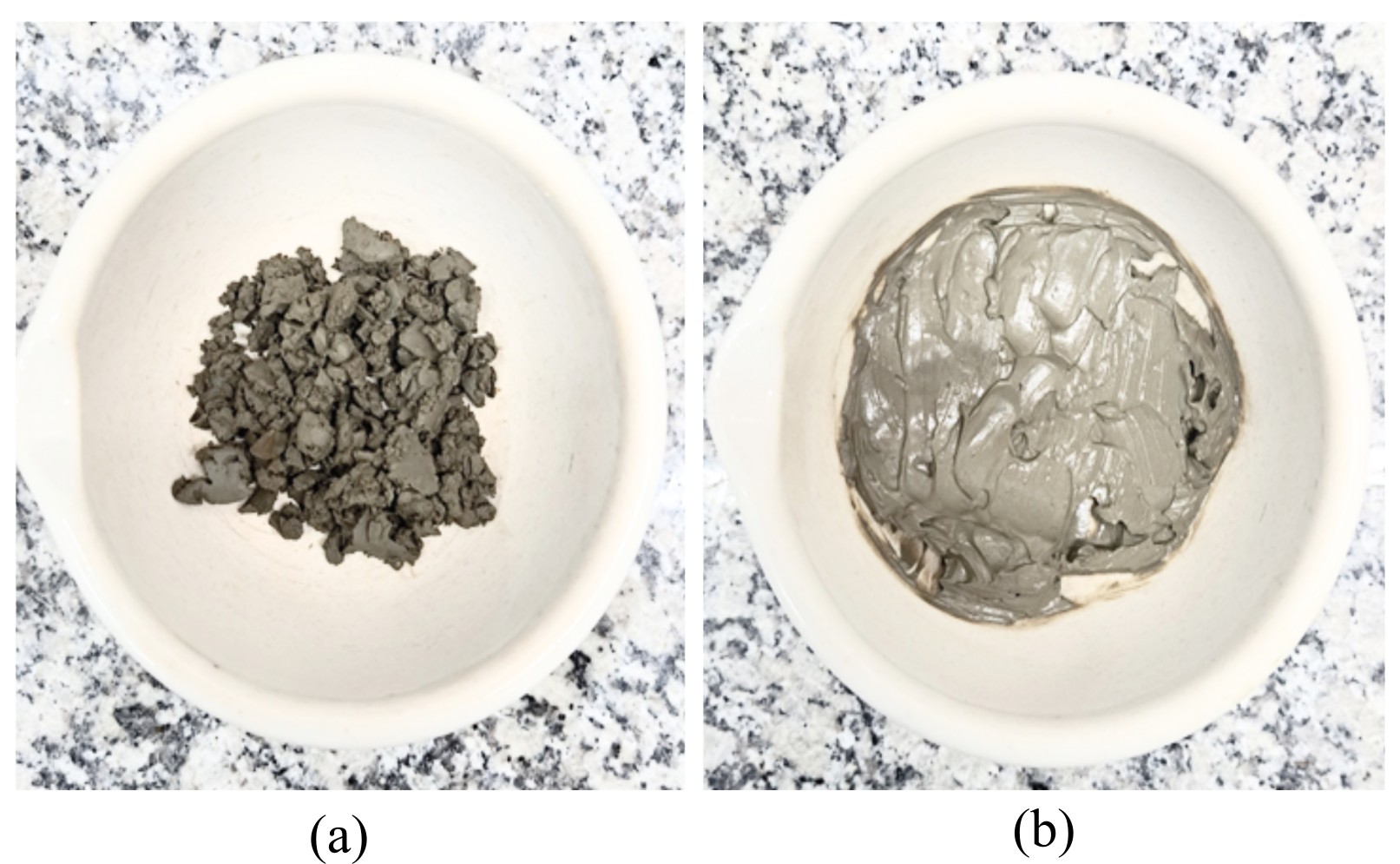
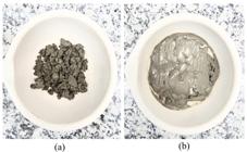
A planetary mechanical mixer was used to homogenize the samples, with a mixing time of 30 minutes for each sample to be tested by adding distilled water. This procedure is necessary to reconstitute the field conditions of the sample in terms of consistency and appropriate water content, as shown in Figure 5a and Figure 5b.

Figure 5
Samples of marine soil: (a) removed from the sampler; (b) homogenized.

Once prepared, the samples were placed in a refrigerator set the test temperature. To prevent water loss during cooling, the containers holding the samples were placed in a sealed bag with a small amount of distilled water sprayed on the bottom. At the start of each test, the sample was removed from the refrigerator, and its temperature was measured using an infrared thermometer with an accuracy of ± 0.1°C and a precision of ± 0.5°C. The measurement procedure consisted of checking three points on the soil surface inside the beaker to ensure temperature uniformity before the rheological test.

3.3 Equipment and test setup

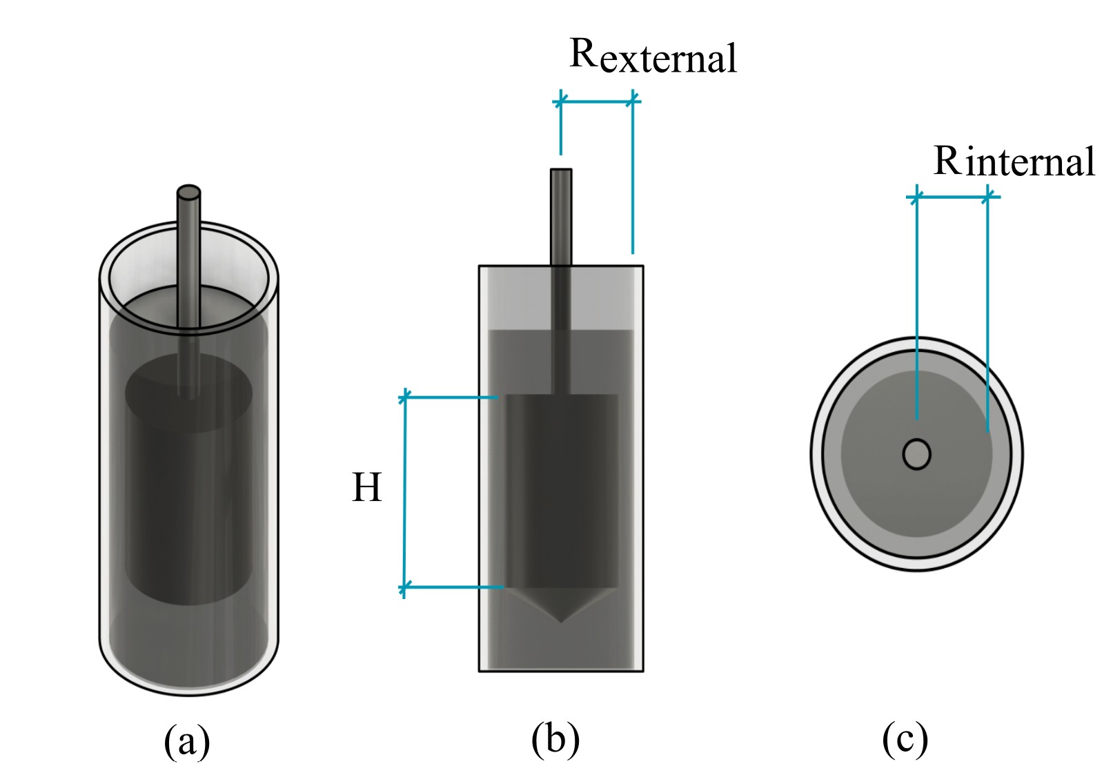
The rheometer used was the RST-CC-SST model, manufactured by Brookfield Viscometers and Rheometers. The tests were conducted using a concentric cylinder geometry. In this setup, the soil sample is placed inside the outer cylinder, as show in Figure 6, with radius R_external. The inner cylinder, with radius R_internal and height H, is then inserted into the system. All dimensions correspond to standard geometries provided by the rheometer manufacturer. In this study, the tests conducted with LI values of 1.1 and 1.5 employed the CCT-25 geometry, whereas those conducted with an LI value of 2.0 employed the CCT-40 geometry. In both cases, the dimensions used correspond to those presented in Table 1.

Figure 6
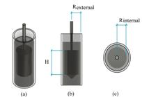
Schematic of the concentric cylinder test: (a) isometric view; (b) front view; (c) top view.

Table 1
Dimensions of the cylinder geometries.

Data	CCT-40	CCT-25
Re – radius of the external cylinder (mm)	21.00	13.56
Ri – radius of the internal cylinder (mm)	3.50	3.50
H – height of the internal cylinder (mm)	60.00	37.50

Important observations regarding the tests are that they are performed using remolded samples, which are carefully placed into the inner cylinder of the rheometer with the aid of a spatula. The tests are conducted under controlled conditions and initiated immediately after sample preparation, once the specimen reaches the target testing temperature.

The equipment was operated in controlled rate (CR) mode, in which the desired shear rate parameters were set, and the corresponding shear stresses were measured. Test programming and data monitoring were performed using the equipment’s proprietary software, Rheo300. Data analysis was carried out using MATLAB and Excel.

At the start of the test, the inner cylinder is rotated from a stationary state, with the shear rate (𝛾̇) increasing linearly from 0 s^-1 to 100 s^-1, while the corresponding shear stress is recorded, this test is called a ramp test. The shear rate range selected was based on studies related to submarine debris flows (Du et al., 2022; Guo et al., 2021; Hotta et al., 2024; Liu et al., 2020a; Shakeel et al., 2022).

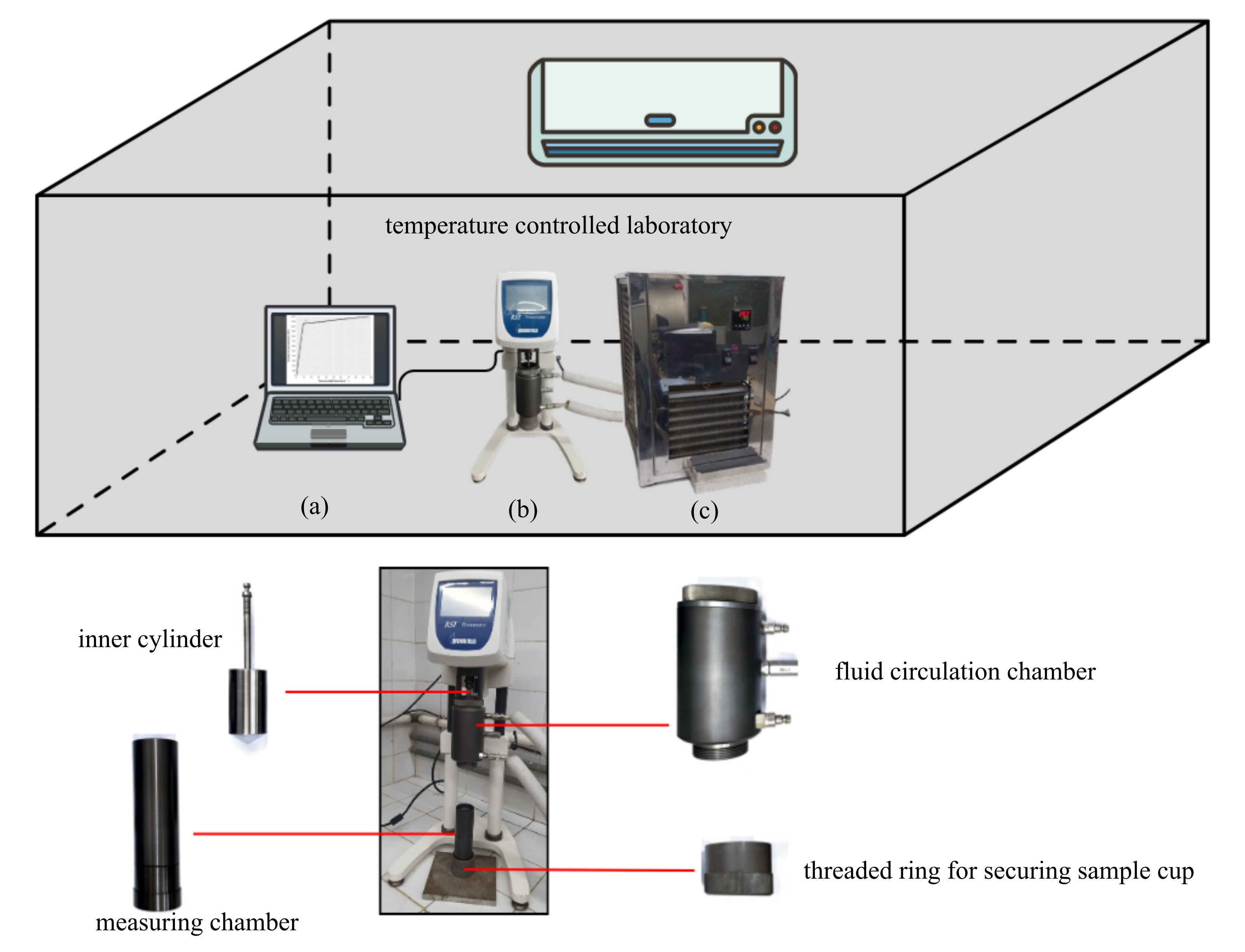
Marine soil samples were tested using concentric cylinder (CC) geometry, targeting LI values of 1.1, 1.5, and 2.0 at controlled temperatures of 6, 13, and 20°C. The test temperature was maintained by circulating a thermostatic fluid through a thermal chamber surrounding the samples. Figure 7 shows the equipment used in the tests.

Figure 7
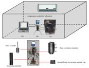
Tests with the rheometer in the laboratory at controlled temperatures: (a) computer system for data acquisition; (b) equipment prepared for testing with the thermostatic fluid inlet and outlet hoses; (c) temperature control and regulation module.

4. Results and discussion

4.1 Geotechnical characterization

The results of the sample characterization tests are listed in Table 2, along with the nomenclature used, location and average depth (below seabed level) of the samples. Analysis of this data revealed that the seabed samples have similar grain size curves, with a predominance of fine fractions (clay, silt and fine sand). According to the Unified Soil Classification System (USCS), all samples were classified as highly compressible inorganic clays (CH).

Table 2
Geotechnical characterization test results.

Sample	Basin	Depth (m)	Clay (%)	Silt (%)	Fine sand (%)	$G_s$	$w_L$ (%)	$w_P$ (%)
S1	Sergipe-Alagoas	30	84	16	0	2.61	73	25
S2		59	72	27	1	2.62	75	24
S3		39	86	14	0	2.70	85	28
S4		44	100	0	0	2.65	55	17
S5		22	80	20	0	2.66	93	31
M1	Campos	49	59	41	0	2.70	70	26
M2		22	37	63	0	2.65	54	20
M3		27	33	66	1	2.65	69	25
M4		39	33	66	1	2.72	69	26
M5		33	47	53	0	2.71	57	31

The marine soil samples analyzed had a liquidity limit of over 54% and plasticity index ranging from 26% to 62%. These values are consistent with those reported in the literature for marine clays (Randolph & Gourvenec, 2017). In addition, the activity index of the clays, according to Skempton’s criteria (1953), indicates that most of the samples studied have normal to inactive behavior.

4.2 Rheological characterization

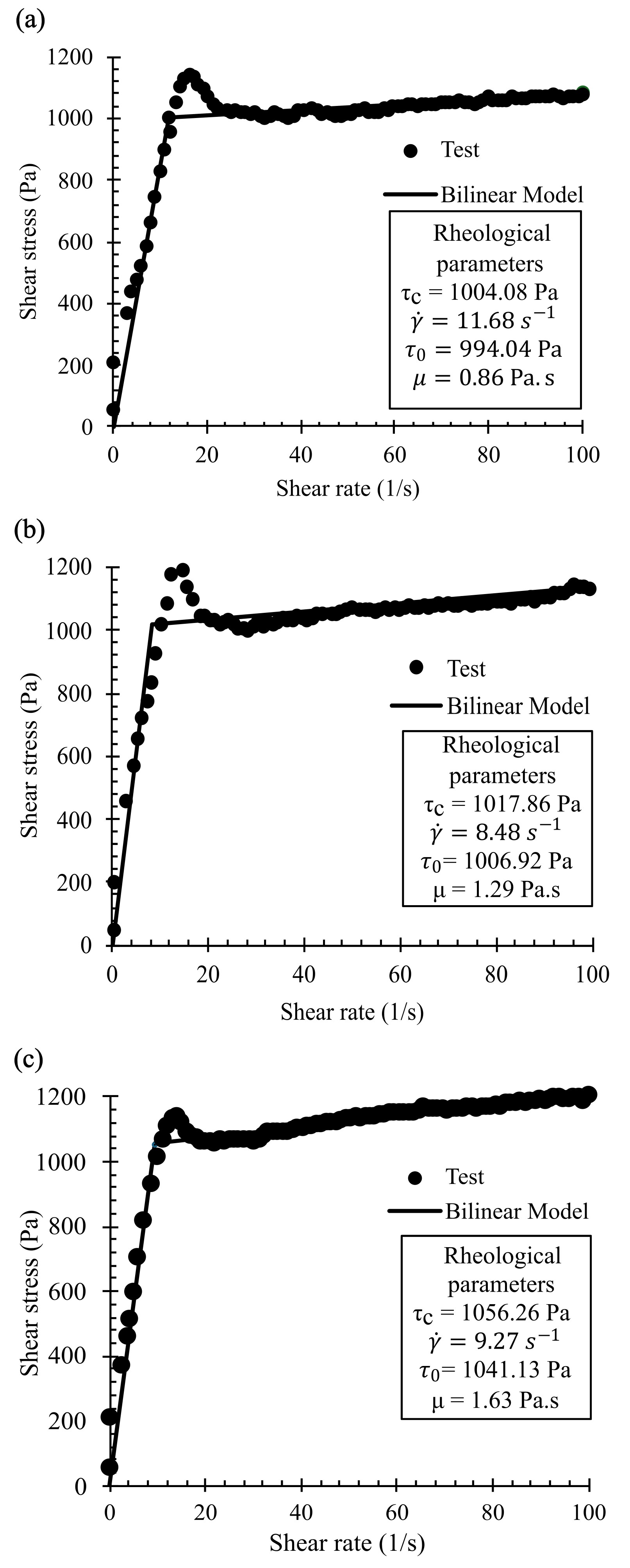
Rheological tests were conducted on each sample, and, by analyzing the flow curves using the Bilinear model, the rheological parameters of the material were obtained at three temperatures (6, 13, and 20°C). Figure 8 shows the results obtained for sample M1 at different temperatures and Liquidity Index (LI) values. The table presented in the Appendix 1 summarizes the rheological parameters obtained for each sample under different test conditions.

Figure 8
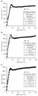
Flow curves and fitted Bilinear model for sample M1: (a) temperature = 20°C and LI = 1.00; (b) temperature =13°C and LI = 1.01; (c) temperature = 6°C and LI = 1.02.

These parameters include yield stress, shear rate and viscosity, which are essential for characterizing the flow behavior of marine soils under varying temperatures and liquidity indices. By comparing the results across tests, it is possible to assess how changes in temperature and water content influence the rheological response of the material, offering insights into its potential behavior in submarine flow scenarios.

The results showed that the yield stress and viscosity increased with decreasing temperature, which is consistent with previous studies (Guo et al., 2020; Nian et al., 2018). However, in contrast to this study, these authors used the Herschel-Bulkley model to determine the rheological parameters.

4.2.1 Correlation of rheological parameters with liquidity index

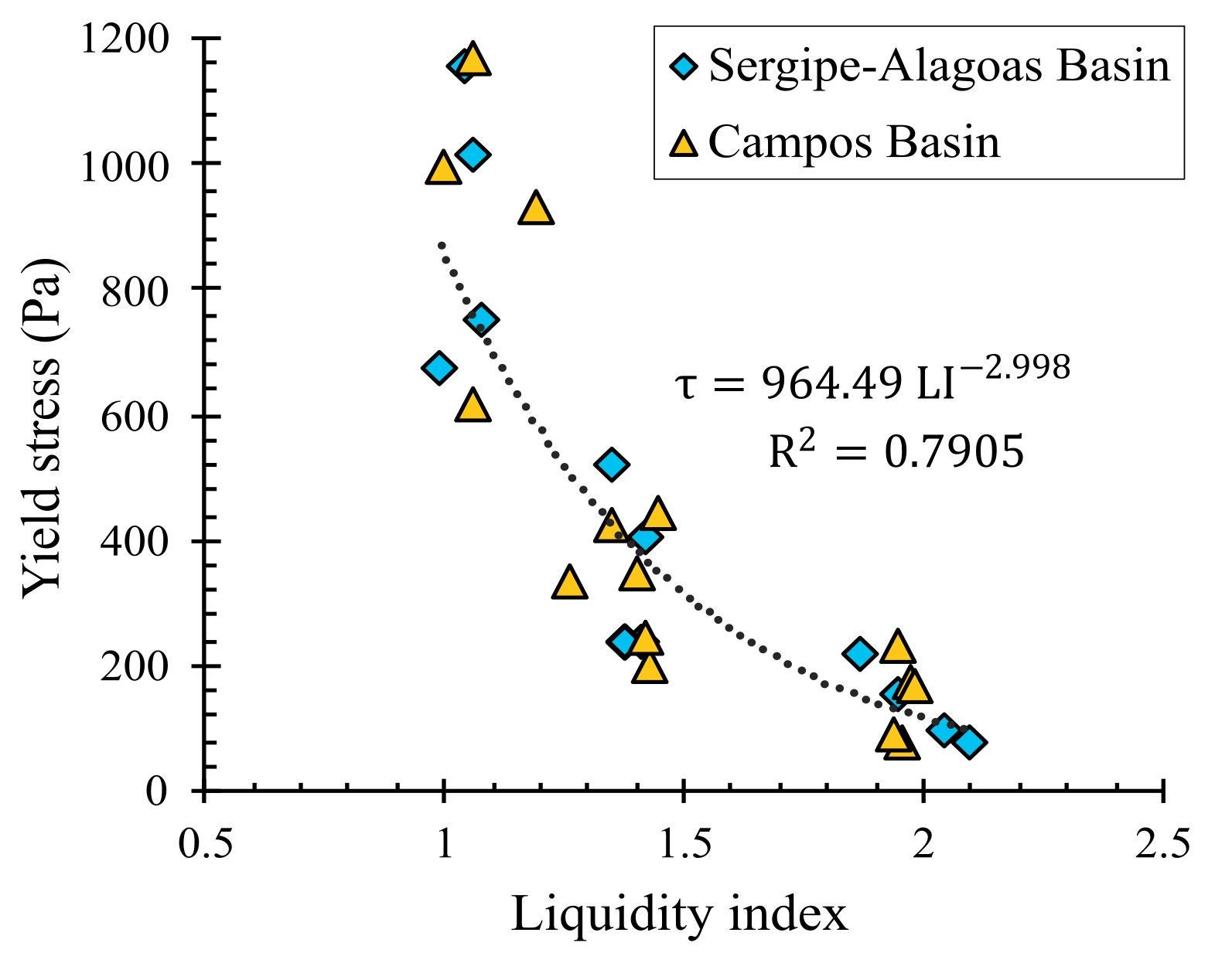
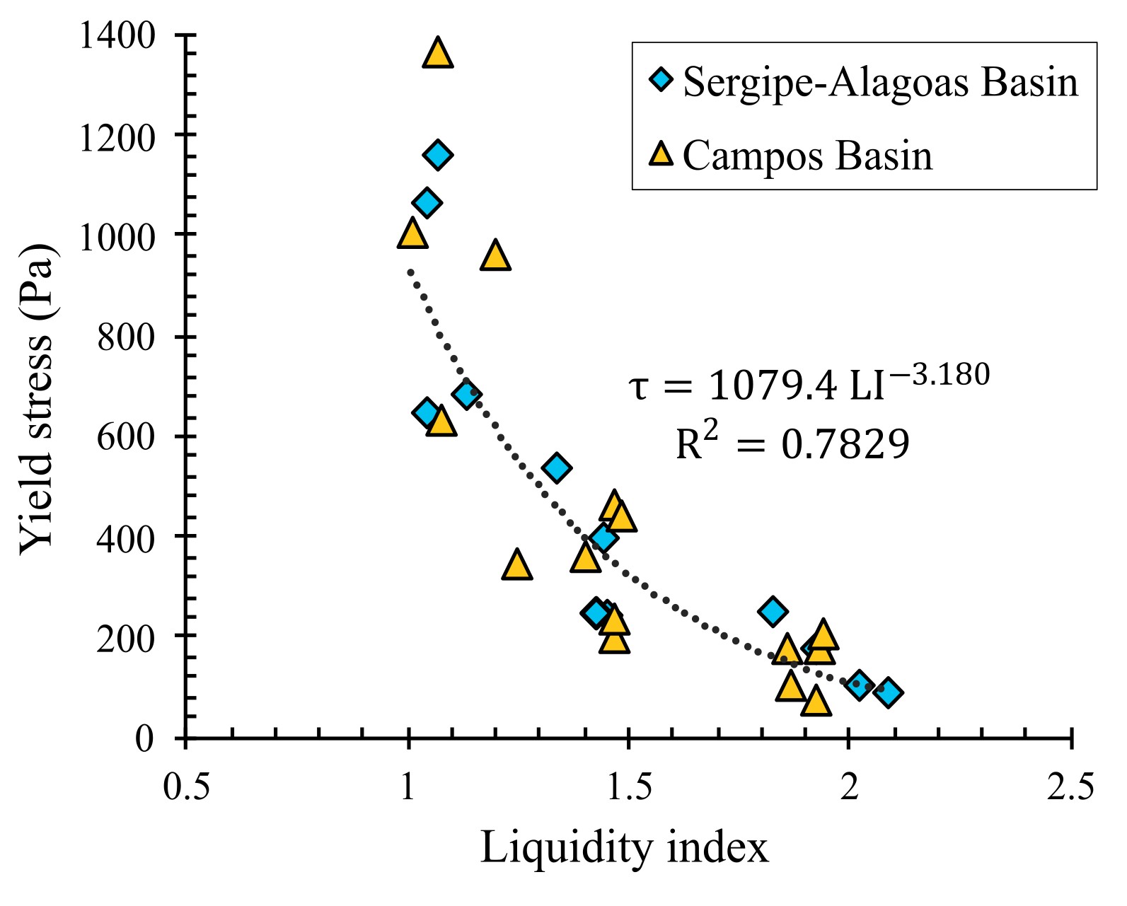
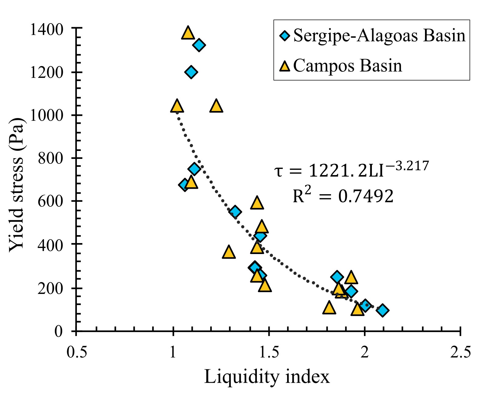
Based on the data obtained and presented in the previous section, the yield stress component of the marine soil accounts for more than 99% of its shear strength, indicating minimal viscosity mobilization in Regime II (Bilinear model). To analyze the influence of temperature, correlation curves were plotted for the yield stress as a function of the liquidity index at 20, 13, and 6°C. The correlation equations presented are expressed in terms of LI, according to the model proposed by Hotta et al. (2024). Figure 9, Figure 10 and Figure 11 illustrate these results.

Figure 9
Correlation curve obtained with the Hotta et al. (2024) model for temperature of 20°C.

Figure 10
Correlation curve obtained with the Hotta et al. (2024) model for temperature of 13°C.

Figure 11
Correlation curve obtained with the Hotta et al. (2024) model for temperature of 6°C.

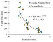
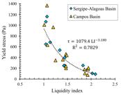
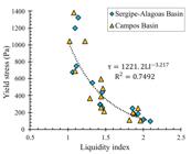
A relevant aspect to be discussed is the coefficient of determination (R²). The results were considered satisfactory as they represented different soil samples collected from various locations across two distinct fields. The data points that lowered the R² values corresponded to liquidity index (LI) values closer to 1; however, these points were important for defining the overall behavior of the curve. This variability reflects the natural heterogeneity of the soil samples and does not undermine the representativeness of our model.

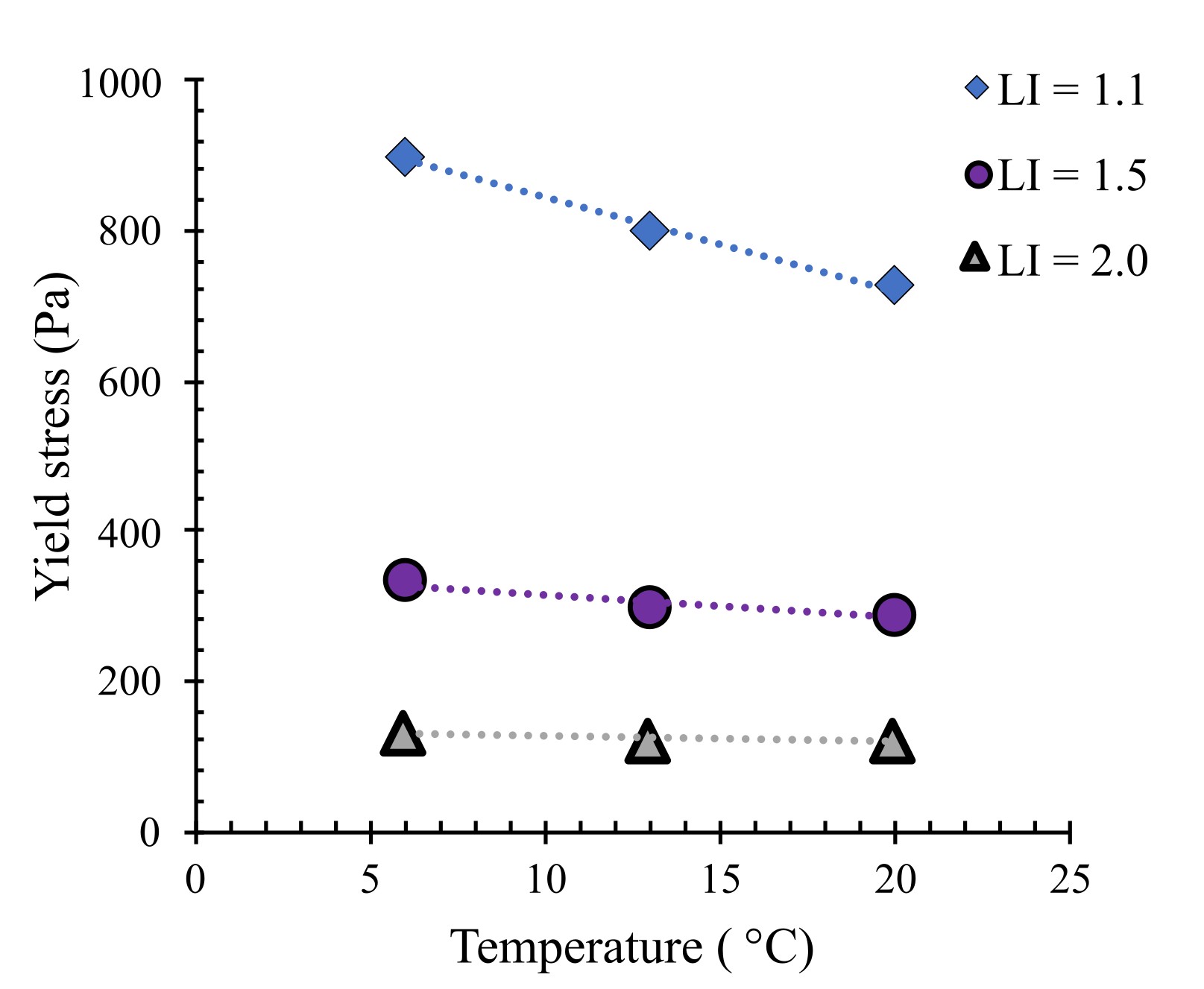
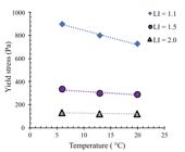
The yield stress behavior of the soil for fixed liquidity indices of 1.1, 1.5, and 2.0—derived from the correlation equations at each temperature—is presented in Figure 12. These LI values were selected solely for visualization. A trend toward linear behavior (yield stress vs. temperature) was observed in all cases, with the slope decreasing as the LI increased. This suggests that temperature has a diminishing influence on the yield stress as the water content of the soil increases. This behavior is attributed to reduced particle-to-particle interactions due to the increased water content in the soil matrix.

Figure 12
Influence of temperature on yield stress in soils with the same liquidity index.

4.2.2 Correlation of rheological parameters with liquidity index and temperature

Based on the discussion presented, a parametric data analysis was conducted to derive an empirical equation for the yield stress as a function of temperature and liquidity index (LI), as shown in Equation 4. The mathematical format indicates an exponential reduction in the yield stress and viscosity, with coefficients that vary linearly, acting both as multipliers of the liquidity index and as its exponent to adjust the behavior as a function of temperature. The coefficients a, b, c, and d are empirical parameters defined by curve fitting.

The coefficient values obtained for the marine soil studied are presented in Equation 5. The linearity of the correlation coefficients can be attributed to thermodynamic principles. Within the tested range, temperature (T) variations led to proportional changes in internal energy and entropy, which affected the mobility of particles in the soil matrix.

$\tau =\left(aT+b\right)L{I}^{-\left(cT+d\right)}$ (4)

$\tau =\left(-18.34T+1326.7\right)L{I}^{-\left(-0.016T+3.34\right)}$ (5)

This process allowed the formulation of a correlation equation that describes the behavior of the soil, considering both the water content and temperature as interdependent factors. Table 3 summarizes of the equations derived from the model by Hotta et al. (2024) and the one proposed in this article.

Table 3
Comparison between models.

Temperature (°C)	Model Hotta et al. (2024)	Proposed model
6	$\tau =1221.20L{I}^{-3.217}$
13	$\tau =1079.40L{I}^{-3.180}$	$\tau =\left(-18.34T+1326.7\right)L{I}^{-\left(-0.016T+3.34\right)}$
20	$\tau =964.49L{I}^{-2.998}$

The results indicate a significant similarity in the values obtained, with a difference of 1.3% compared with the model by Hotta et al. (2024). This consistency suggests that the model proposed in this study can be a reliable tool for analyses that incorporate the influence of temperature.

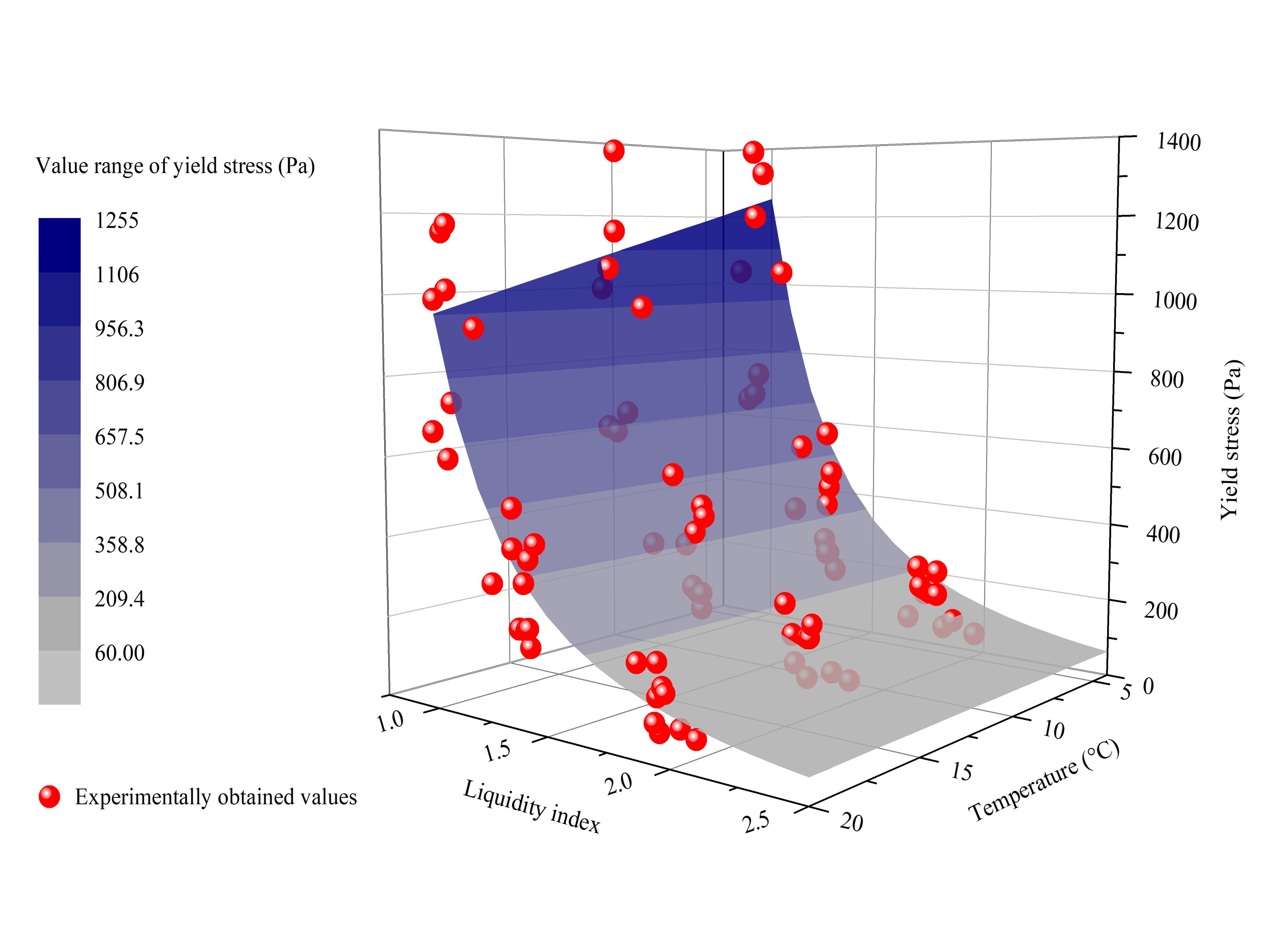
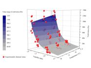
Based on these results, it is useful to represent the yield surface for the marine soil (Figure 13), which is a graph that relates the axes of temperature, liquidity index and apparent yield stress. This representation demonstrates how the rheological properties of the soil change and how these changes occur in relation to the parameters studied.

Figure 13
Representations of the yield surface studied.

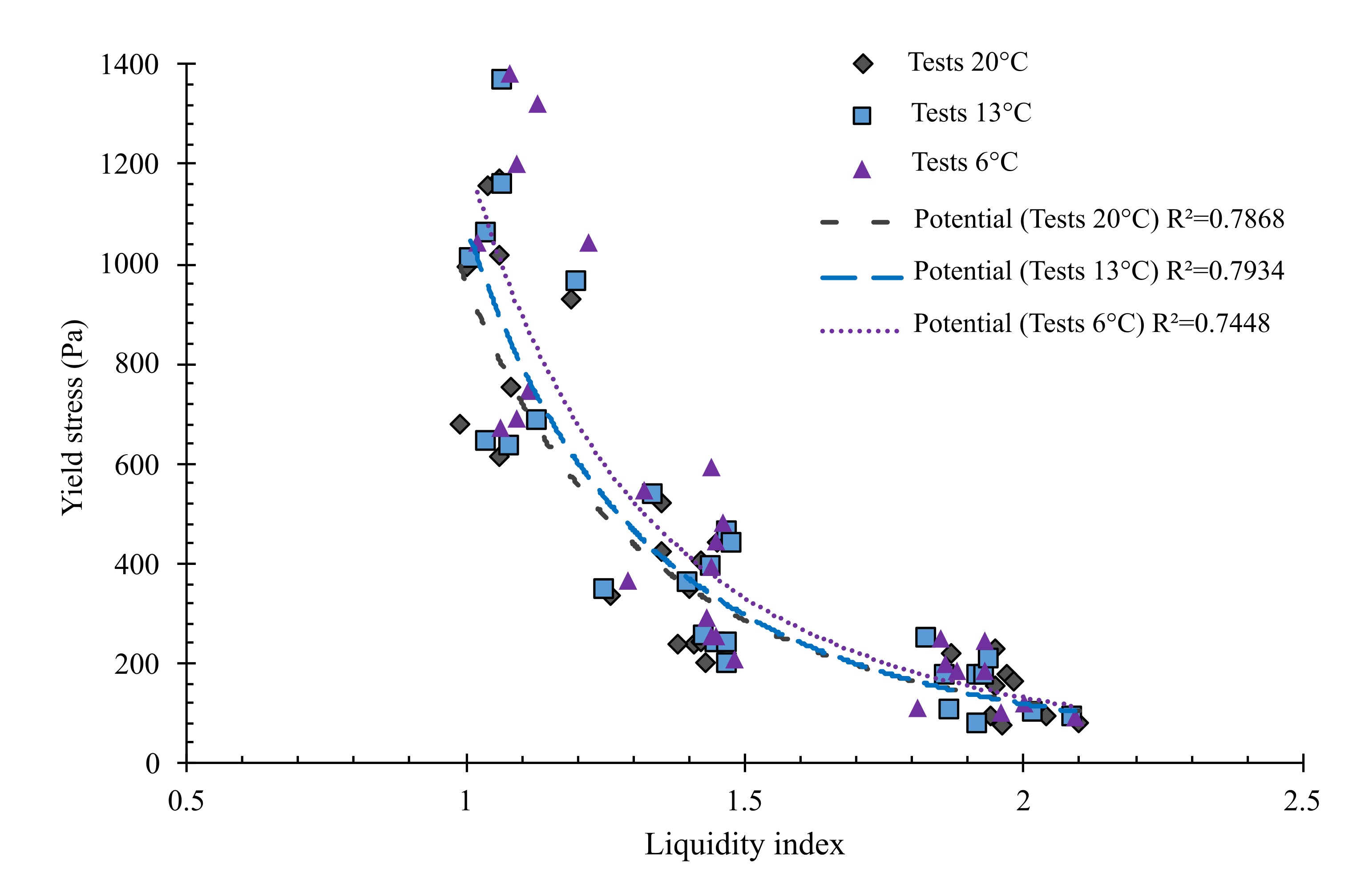
Three sections were defined on the liquidity index vs. yield stress plane, corresponding to the tested temperatures of 6, 13, and 20°C, and the resulting correlation curves are shown in Figure 14. The experimental data were in agreement with the exponential fitting curves, as indicated by the satisfactory R² values. These results demonstrate that the model effectively accounts for the temperature influence. Furthermore, when the three curves are displayed on the same graph, an increase in soil resistance with decreasing temperature becomes evident—an effect that is more pronounced for liquidity index values near 1, as previously discussed.

Figure 14
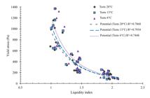
Correlation curve obtained with the proposed model for temperatures of 6°C, 13°C, and 20°C.

5. Conclusions

This study contributes to a better understanding of the rheological behavior of marine soils under submarine debris flow conditions, a phenomenon of great relevance for the safety of offshore infrastructure and mitigating environmental impacts. The main objective was to develop a predictive model that correlates the yield stress with the liquidity index and temperature, enabling a more accurate representation of soil behavior under varying physical conditions.

The experimental results confirmed that temperature directly influences the rheological response of marine soils. The yield stress accounted for more than 99% of the shear strength of the samples. Additionally, it was observed that the influence of temperature diminishes as the water content in the soil increases. From a thermodynamic perspective, temperature is a measure of the average kinetic energy of particles. As the temperature decreases, the kinetic energy diminishes, leading to a reduction in the intensity of Brownian motion. This reduction affects the microstructure of the soil by increasing particle interactions and flocculation tendencies, which in turn elevates the yield stress. Additionally, temperature variations influence the viscosity of the pore water, which tends to increase as the temperature decreases, thus contributing to higher resistance against deformation. The observed linear reduction in yield stress with increasing temperature can be attributed to the combined effects of diminishing particle agitation and changes in fluid viscosity, which together modulate the flow behavior of the soil.

Based on these findings, a predictive model was developed that incorporated both liquidity index and temperature. The proposed formulation offers a practical and theoretically grounded tool for improving the reliability of geotechnical assessments involving marine soils under low-temperature conditions, with direct application in the context of submarine debris flows. The correlation equations established in this study allow the use of laboratory results obtained at offshore ambient temperatures to model submarine debris flows occurring at different depths, since seawater temperature decreases with increasing depth.

The proposed relationships are intended to represent soil behavior during flow and to support numerical simulations aimed at predicting the dynamics of submarine debris flows, in which knowledge of the rheological parameters is fundamental to predict the response of the soil under hydrodynamic conditions. It is important to note that these results are not intended for applications related to soil mechanics approaches focused on slope stability analyses, as the tests were conducted on remolded samples and specifically designed to investigate soil behavior under flow conditions rather than failure initiation.

List of symbols

$a$ Empirical parameters

$b$ Empirical parameter

c Empirical parameter

$d$ Empirical parameters

$\text{AABW}$ Antarctic Bottom Water

$\text{AAIW}$ Antarctic Intermediate

$\text{CC}$ Concentric cylinder

$\text{CH}$ Highly compressible inorganic clays

$\text{CR}$ Controlled rate

$G_s$ Specific gravity of soils

$H$ Height of the internal cylinder

$\text{LCDW}$ Lower Circumpolar Deep Water

$\text{LI}$ Liquidity index

$\text{NADW}$ North Atlantic Deep Water

$R_e$ Radius of the external cylinder

$R_i$ Radius of the internal cylinder

$R²$ Coefficient of determination

$\text{SACW}$ South Atlantic Central Water

$T$ Temperature

$\text{TW}$ Tropical Water

$\text{UCDW}$ Upper Circumpolar Deep Water

$\text{USCS}$ Unified Soil Classification System

$w$ Water content

$w_P$ Water content at plastic limit

$w_L$ Water content at liquid limit

$\dot{\gamma }$ Shear rate

${\dot{\gamma }}_c$ Critical shear rate

$\mu$ Viscosity

${\mu }_1$ Regime I viscosity

${\mu }_2$ Regime II viscosity

$\tau$ Shear stress of the material

${\tau }_0$ Yield stress

${\tau }_c$ Critical yield stress

Appendix 1 Rheological parameters obtained for all samples using the Bilinear model.

Sample	Temperature = 20°C				Temperature = 13°C				Temperature = 6°C
	${\tau }_0$ (Pa)	$\mu$ (Pa.$s$)	${\dot{\gamma }}_c$ ($1/s$)	LI	${\tau }_0$ (Pa)	$\mu$ (Pa.$s$)	${\dot{\gamma }}_c$ ($1/s$)	LI	${\tau }_0$ (Pa)	$\mu$ (Pa.$s$)	${\dot{\gamma }}_c$ ($1/s$)	LI
S1	1017.75	2.47	7.26	1.06	1059.91	1.48	8.68	1.04	1321.29	3.39	9.87	1.13
	518.75	0.73	10.24	1.35	532.47	0.94	8.15	1.34	546.88	1.95	7.34	1.32
	219.34	0.24	7.60	1.87	247.06	0.16	6.99	1.83	250.98	5.63	5.63	1.85
S3	676.44	1.71	8.61	0.99	640.28	1.76	10.94	1.04	673.02	2.59	10.28	1.06
	238.41	0.31	8.44	1.41	237.37	0.46	7.02	1.45	254.00	0.73	6.48	1.45
	94.61	0.12	5.18	2.04	98.68	0.17	4.95	2.02	119.38	0.17	5.03	2.00
S4	750.72	1.43	11.28	1.08	683.00	0.88	10.94	1.13	745.61	1.61	10.24	1.11
	238.32	0.31	8.45	1.38	249.97	0.25	7.45	1.43	290.07	0.24	8.79	1.43
	80.49	0.01	6.69	2.10	87.08	0.02	5.76	2.09	93.21	0.00	5.44	2.09
S5	1153.68	1.42	14.33	1.04	1156.37	2.44	10.51	1.07	1198.95	2.31	10.73	1.09
	404.35	0.54	10.68	1.42	390.99	0.89	7.66	1.44	441.75	1.04	9.35	1.45
	152.72	0.15	9.35	1.95	171.26	0.17	9.37	1.92	182.76	0.18	7.10	1.93
M1	994.04	0.86	11.68	1.00	1006.92	1.29	8.48	1.01	1041.13	1.63	9.27	1.02
	347.23	0.02	7.38	1.40	356.47	0.06	7.92	1.40	390.56	0.25	5.41	1.44
	177.02	0.01	9.63	1.97	173.26	0.02	6.64	1.86	182.59	0.04	6.37	1.88
M2	930.55	1.86	12.91	1.19	961.24	2.16	10.85	1.20	1040.75	3.04	10.09	1.22
	423.40	1.19	7.66	1.35	460.73	1.19	8.49	1.47	591.43	1.48	7.39	1.44
	164.44	0.22	8.20	1.98	172.35	0.29	5.52	1.93	199.63	0.34	7.45	1.86
M3	332.70	0.24	10.82	1.26	344.64	0.65	9.86	1.25	366.13	0.73	9.45	1.29
	200.00	0.16	9.19	1.43	197.23	0.22	9.16	1.47	208.19	0.36	8.43	1.48
	75.20	0.03	6.25	1.96	73.47	0.05	4.10	1.92	110.34	0.13	8.31	1.81
M4	1171.30	1.90	10.31	1.06	1364.98	2.28	9.09	1.07	1382.74	3.07	6.99	1.08
	442.69	0.16	6.37	1.45	434.90	0.54	5.56	1.48	481.52	0.95	3.41	1.46
	229.61	0.02	7.18	1.95	205.32	0.05	4.06	1.94	245.78	0.16	5.40	1.93
M5	614.72	0.96	11.87	1.06	630.58	1.11	11.13	1.08	687.91	0.65	9.75	1.09
	242.25	0.11	9.55	1.42	235.64	0.19	8.44	1.47	253.40	0.34	7.11	1.44
	93.38	0.06	9.11	1.94	103.78	0.04	6.55	1.87	98.34	0.07	4.33	1.96

Acknowledgements

Their authors would like to express their gratitude to the staff of the LM²C at COPPE/UFRJ for their support in conducting the test program presented in this study. This research is part of a collaborative effort between Petrobras and the Federal University of Rio de Janeiro.

• Discussion open until November 30, 2026.
• Declaration of use of generative artificial intelligence
  This work was prepared with the assistance of generative artificial intelligence (GenAI) Deepl Write with the aim of reviewing the translation in English. The entire process of using this tool was supervised, reviewed and when necessary edited by the authors. The authors assume full responsibility for the content of the publication that involved the aid of GenAI.

Data availability

The datasets generated and analyzed during the present study are available from the corresponding author upon reasonable request.

References

• ASTM D7928-17. (2017). Standard Test Method for Particle-Size Distribution (Gradation) of Fine-Grained Soils Using the Sedimentation (Hydrometer) Analysis ASTM International, West Conshohocken, PA. https://doi.org/10.1520/D7928-17
  » https://doi.org/10.1520/D7928-17
• ASTM D4318-17e1. (2018). Standard Test Methods for Liquid Limit, Plastic Limit, and Plasticity Index of Soils ASTM International, West Conshohocken, PA.https://doi.org/10.1520/D4318-17E01
  » https://doi.org/10.1520/D4318-17E01
• ASTM D6913/D6913M-17. (2021). Standard Test Methods for Particle Size Distribution (Gradation) of Soils Using Sieve Analysis ASTM International, West Conshohocken, PA. https://doi.org/10.1520/D6913_D6913M-17
  » https://doi.org/10.1520/D6913_D6913M-17
• Barnes, H.A., Hutton, J.F., & Walters, K. (2005). An introduction to rheology, Transferred to digital printing Elsevier.
• Carneiro, M.E.R., Fontes, L.C.S., & Bernabéu, A.P. (2017). Geologia e geomorfologia da bacia de Sergipe-Alagoas Fundação Universidade Federal de Sergipe (in Portuguese).
• Du, J., Choi, C.E., Yu, J., & Thakur, V. (2022). Mechanisms of submarine debris flow growth. Journal of Geophysical Research. Earth Surface, 127(2), e2021JF006470. https://doi.org/10.1029/2021JF006470
  » https://doi.org/10.1029/2021JF006470
• Fan, N., Jiang, J., Dong, Y., Guo, L., & Song, L. (2022). Approach for evaluating instantaneous impact forces during submarine slide-pipeline interaction considering the inertial action. Ocean Engineering, 245, 110466. https://doi.org/10.1016/j.oceaneng.2021.110466
  » https://doi.org/10.1016/j.oceaneng.2021.110466
• Figueiredo, A.G., Pacheco, C.E.P., De Vasconcelos, S.C., & Da Silva, F.T. (2015). Geomorfologia e sedimentologia da plataforma continental. In R. O. Kowsmann (Ed.), Geologia e geomorfologia (pp. 13-32). Elsevier. https://doi.org/10.1016/B978-85-352-6937-6.50009-4
  » https://doi.org/10.1016/B978-85-352-6937-6.50009-4
• Guo, X., Nian, T., Gu, Z., Li, D., Fan, N., & Zheng, D. (2021). Evaluation methodology of laminar-turbulent flow state for fluidized material with special reference to submarine landslide. Journal of Waterway, Port, Coastal, and Ocean Engineering, 147(1), 04020048. https://doi.org/10.1061/(ASCE)WW.1943-5460.0000616
  » https://doi.org/10.1061/(ASCE)WW.1943-5460.0000616
• Guo, X., Zheng, D., Nian, T., & Lv, L. (2020). Large-scale seafloor stability evaluation of the northern continental slope of South China Sea. Marine Georesources and Geotechnology, 38(7), 804-817. https://doi.org/10.1080/1064119X.2019.1632996
  » https://doi.org/10.1080/1064119X.2019.1632996
• Halliday, D. (2022). Fundamentos de física - gravitação, ondas e termodinâmica - volume dois LTC-Livros Tecnicos E Cientificos Editora Lda (in Portuguese).
• Hotta, M.M., Almeida, M.S.S., Oliveira, J.R.M.S., & Borges, R.G. (2024). Study of the influence of rheological parameters on the behavior of a submarine debris flow. Soil and Rocks, 47(4), e2024001524. https://doi.org/10.28927/SR.2024.001524
  » https://doi.org/10.28927/SR.2024.001524
• Jeong, S.W. (2014). The effect of grain size on the viscosity and yield stress of fine-grained sediments. Journal of Mountain Science, 11(1), 31-40. https://doi.org/10.1007/s11629-013-2661-1
  » https://doi.org/10.1007/s11629-013-2661-1
• Kaminski, P., Sager, T., Grabe, J., & Urlaub, M. (2021). A new methodology to assess the potential of conjectural trigger mechanisms of submarine landslides exemplified by marine gas occurrence on the Balearic Promontory. Engineering Geology, 295, 106446. https://doi.org/10.1016/j.enggeo.2021.106446
  » https://doi.org/10.1016/j.enggeo.2021.106446
• Leffler, W.L., Pattarozzi, R., & Sterling, G. (2011). Deepwater petroleum exploration & production: a nontechnical guide PennWell Corp.
• Lima, L.B.D., Hotta, M.M., Takayassu, L.C., Nunes, P., Almeida, M.D.S.S., & Borges, R.G. (2024). Estudo comparativo entre ensaios de palheta e cilindros concêntricos com amostras de argila marinha utilizando o reômetro de bancada. In Proceedings of the 8th Congresso Brasileiro de Mecânica dos Solos e Engenharia Geotécnica Recife. Editora OMNIS Scientia. (in Portuguese). https://doi.org/10.47094/COBRAMSEG2024/623
  » https://doi.org/10.47094/COBRAMSEG2024/623
• Liu, D., Cui, Y., Guo, J., Yu, Z., Chan, D., & Lei, M. (2020a). Investigating the effects of clay/sand content on depositional mechanisms of submarine debris flows through physical and numerical modeling. Landslides, 17(8), 1863-1880. https://doi.org/10.1007/s10346-020-01387-6
  » https://doi.org/10.1007/s10346-020-01387-6
• Liu, F., Tan, L., Crosta, G., & Huang, Y. (2020b). Spatiotemporal destabilization modes of upper continental slopes undergoing hydrate dissociation. Engineering Geology, 264, 105286. https://doi.org/10.1016/j.enggeo.2019.105286
  » https://doi.org/10.1016/j.enggeo.2019.105286
• Locat, J., & Lee, H. (2009). Submarine mass movements and their consequences: an overview. In K. Sassa & P. Canuti (Eds.), Landslides – Disaster Risk Reduction (pp. 115-142). Springer. https://doi.org/10.1007/978-3-540-69970-5_6
  » https://doi.org/10.1007/978-3-540-69970-5_6
• Locat, J., & Lee, H.J. (2002). Submarine landslides: advances and challenges. Canadian Geotechnical Journal, 39(1), 193-212. https://doi.org/10.1139/t01-089
  » https://doi.org/10.1139/t01-089
• Masson, D.G., Harbitz, C.B., Wynn, R.B., Pedersen, G., & Løvholt, F. (2006). Submarine landslides: processes, triggers and hazard prediction. Philosophical Transactions. Series A, Mathematical, Physical, and Engineering Sciences, 364(1845), 2009-2039. PMid:16844646. https://doi.org/10.1098/rsta.2006.1810
  » https://doi.org/10.1098/rsta.2006.1810
• Meinen, C.S., Perez, R.C., Dong, S., Piola, A.R., & Campos, E. (2020). Observed ocean bottom temperature variability at four sites in the northwestern Argentine basin: evidence of decadal deep/abyssal warming amidst hourly to interannual variability during 2009–2019. Geophysical Research Letters, 47(18), e2020GL089093. https://doi.org/10.1029/2020GL089093
  » https://doi.org/10.1029/2020GL089093
• Meng, Q., Liu, S., Jia, Y., Xiao, Z., & Wang, X. (2018). Analysis on acoustic velocity characteristics of sediments in the northern slope of the South China Sea. Bulletin of Engineering Geology and the Environment, 77(3), 923-930. https://doi.org/10.1007/s10064-017-1070-z
  » https://doi.org/10.1007/s10064-017-1070-z
• Messaoudi, A., Bouzit, M., & Boualla, N. (2018). Physical and rheological properties of the Chorfa dam mud: dependency on solids concentration. Applied Water Science, 8(6), 178. https://doi.org/10.1007/s13201-018-0805-8
  » https://doi.org/10.1007/s13201-018-0805-8
• Morais, J.M. (2013). Petróleo em águas profundas: uma história tecnológica da PETROBRAS na exploração e produção offshore Ipea (in Portuguese).
• Mosher, D.C., Shipp, R.C., Moscardelli, L., Chaytor, J.D., Baxter, C.D.P., Lee, H.J., & Urgeles, R. (Eds.) (2010). Submarine mass movements and their consequences Springer. https://doi.org/10.1007/978-90-481-3071-9
  » https://doi.org/10.1007/978-90-481-3071-9
• Mothe, C.G. (2006.) Reologia e reometria - Fundamentos teóricos e práticos Artliber (in Portuguese).
• Nian, T., Guo, X., Fan, N., Jiao, H., & Li, D. (2018). Impact forces of submarine landslides on suspended pipelines considering the low-temperature environment. Applied Ocean Research, 81, 116-125. https://doi.org/10.1016/j.apor.2018.09.016
  » https://doi.org/10.1016/j.apor.2018.09.016
• Nian, T., Guo, X., Zheng, D., Xiu, Z., & Jiang, Z. (2019). Susceptibility assessment of regional submarine landslides triggered by seismic actions. Applied Ocean Research, 93, 101964. https://doi.org/10.1016/j.apor.2019.101964
  » https://doi.org/10.1016/j.apor.2019.101964
• Nie, S., Jiang, Q., Cui, L., & Zhang, C. (2020). Investigation on solid-liquid transition of soft mud under steady and oscillatory shear loads. Sedimentary Geology, 397, 105570. https://doi.org/10.1016/j.sedgeo.2019.105570
  » https://doi.org/10.1016/j.sedgeo.2019.105570
• Randolph, M., & Gourvenec, S. (2017). Offshore geotechnical engineering CRC Press.
• Rui, Y., & Yin, M. (2019). An Analytical solution for the run-out of submarine debris flows. Marine Geodesy, 42(3), 246-262. https://doi.org/10.1080/01490419.2019.1583146
  » https://doi.org/10.1080/01490419.2019.1583146
• Schambach, L., Grilli, S.T., Tappin, D.R., Gangemi, M.D., & Barbaro, G. (2020). New simulations and understanding of the 1908 Messina tsunami for a dual seismic and deep submarine mass failure source. Marine Geology, 421, 106093. https://doi.org/10.1016/j.margeo.2019.106093
  » https://doi.org/10.1016/j.margeo.2019.106093
• Shakeel, A., Zander, F., De Klerk, J.-W., Kirichek, A., Gebert, J., & Chassagne, C. (2022). Effect of organic matter degradation in cohesive sediment: a detailed rheological analysis. Journal of Soils and Sediments, 22(11), 2883-2892. https://doi.org/10.1007/s11368-022-03156-5
  » https://doi.org/10.1007/s11368-022-03156-5
• Tsugawa, J.K., Romano, R.C. O., Pileggi, R.G., & Boscov, M.E.G. (2019). Review: rheology concepts applied to geotechnical engineering. Applied Rheology (Lappersdorf, Germany), 29(1), 202-221. https://doi.org/10.1515/arh-2019-0018
  » https://doi.org/10.1515/arh-2019-0018
• Urgeles, R., & Camerlenghi, A. (2013). Submarine landslides of the Mediterranean Sea: trigger mechanisms, dynamics, and frequency-magnitude distribution. Journal of Geophysical Research: Earth Surface, 118(4), 2600-2618. https://doi.org/10.1002/2013JF002720
  » https://doi.org/10.1002/2013JF002720
• Wang, H., Cui, P., Li, Y., Tang, J., Wei, R., Yang, A., Zhou, L., Bazai, N.A., & Zhang, G. (2024). Rock and ice avalanche-generated catastrophic debris flow at Chamoli, 7 February 2021: new insights from the geomorphic perspective. Geomorphology, 452, 109110. https://doi.org/10.1016/j.geomorph.2024.109110
  » https://doi.org/10.1016/j.geomorph.2024.109110

Edited by

• Editor:
  Renato P. Cunha https://orcid.org/0000-0002-2264-9711

Publication Dates

• Publication in this collection
  06 July 2026
• Date of issue
  2026

History

• Received
  16 Apr 2025
• Accepted
  20 Mar 2026