Solving Weighted Orthogonal Procrustes Problems via a Projected Gradient Method

ABSTRACT

This paper proposes a family of line-search methods to deal with weighted orthogonal procrustes problems. In particular, the proposed family uses a search direction based on a convex combination between the Euclidean gradient and the Riemannian gradient of the cost function. The non-monotone line-search of Zhang and Hager, and an adaptive Barzilai-Borwein step-size are the chosen tools, in order to speed up the convergence of the new family of methods. One of the extremes of that convex combination is reduced to well-known spectral projected gradient method, while the another one can be interpreted as a Riemannian steepest descent method. To preserve feasibility of all the iterates, we use a projection operator based on the singular value decomposition, which can be computed efficiently via the spectral decomposition of an appropriate matrix. In addition, we prove that the entire uncountable collection of search directions satisfies a descent condition. Some numerical experiments are provided in order to demonstrate the effectiveness of the new approach.

Keywords:
continuous optimization; constrained optimization; Stiefel manifold; procrustes analysis; projected gradient method

1 INTRODUCTION

In this paper, we consider the following equality constrained least-square problem

$\underset{X\in {\mathrm{ℝ}}^{m\times n}}{min}\frac{1}{2}{||AXC-B||}_F^2,subjectto{X}^{\top }X=I,$ (1.1)

where n≤m, A∈ℝ^p×m , B∈ℝ^p×q and C∈ℝ^n×q are three given data matrices. This optimization problem is known as the weighted orthogonal procrustes problem (WOPP)^{21), (23}. The set formed by the constraints, that is St(m, n):={X∈ℝ^m×n: X ^⊤ X=I} is called the Stiefel manifold⁶. The Stiefel manifold is a compact set, which guarantees that (1.1) has at least a global optimum. This set can be regarded as an embedded Riemannian sub-manifold of ℝ^m×n with dimension equals to $mn-\frac{1}{2}n\left(n+1\right)$, see¹.

The optimization model (1.1) has many applications such as, body rigid movements²², psychometry⁹, global positioning system³ and trace minimization²⁴. In addition, some dimension reduction techniques very useful in statistical pattern recognition such as laplacean eigenmaps, locality preserving projections, orthogonal neighborhood preserving projection, orthogonal locality preserving projections can be posed as problem (1.1), for details see¹¹.

Some special cases of the non-convex quadratic optimization problem with quadratic equality constraints (1.1) have closed expressions for their solution. In particular, if B=0 and C=I _{n, q} (i.e. the rectangular diagonal matrix with diagonal entries equal one) then any global solution correspond to a matrix X* whose columns span the eigenspace of A ^⊤ A associated with the n-smallest eigenvalues of A ^⊤ A, and the optimal value is $0.5{||AX||}_F^2=\left({\Sigma }_{i=1}^n{\lambda }_i\right)/2$, where λ₁≤λ₂≤...λ_m denotes the eigenvalues of A ^⊤ A. In addition, if C=I _{n, q} , and m=n then the optimization problem (1.1) is known as the orthogonal procrustes problem (OPP)^{21), (23), (28} or also balanced procrustes problem²⁸ and an explicit solution can be derived by using the singular value decomposition (SVD) of B ^⊤ A^{21), (23}. The general case when C=I _{n, q} , and n<mml:m is known as unbalanced procrustes problem²⁸. Unfortunately, both the unbalanced procrustes problem and the weighted version of the orthogonal procrustes problem, i.e. the optimization model (1.1) do not have closed expressions for their solutions. Moreover, compute a solution of the more general problem (1.1) is a costly task, due to the non-linearity and non-convexity of the constraints set St(m, n), which may generate that the WOPP problem have multiple local or global solutions. In fact, Viklands in²³ conjectured that the WOPP problem has at most 2ⁿ unconnected minima. Therefore, a solution is possible only computationally by using an iterative procedure. There are several iterative algorithms, in the literature, that can be used to solve the problem (1.1), see^{8), (13), (15), (16), (18), (20), (25), (29}. The vast number of applications of the optimization problem (1.1) and the difficulty to solve it motivates the design of new iterative methods to obtain approximations of at least its local minimizers.

In this paper, we develop a new iterative algorithm to tackle the optimization problem (1.1). In particular, we design a new projected gradient-type method, which uses a search direction based on a convex combination between the Euclidean gradient and the Riemannian gradient of the quadratic cost function. To improve the efficiency of the method, we consider a self-adaptive step size based on the Barzilai-Borwein step sizes, in combination with an inaccurate non-monotone line-search. In order to preserve the feasibility of all the iterates, we use the standard projection operator on the Stiefel manifold. Finally, we present some numerical experiments to illustrate the efficacy and fast convergence of the new approach.

This paper is organized as follows. In the next section, we present some notations and tools necessary for a good understanding of this paper. In subsection 2.1, we establishes the first-order necessary optimality conditions corresponding with (1.1). Section 3 exhibits our proposed algorithm, and comment its convergence properties. Section 4 presents some numerical results. Finally, we provide the conclusions in Section 5.

2 NOTATIONS AND TOOLS

In the rest of the present manuscript, we say that W∈ℝ^n×n is skew-symmetric if W=-W ^⊤. The expression ℳ_n (ℝ^m×n ) will be denote the following set ℳ_n (ℝ^m×n ):={X∈ℝ^m×n: rank(X)=n}, where rank(X) denotes the rank of the matrix X. The objective function of problem (1.1) will be denoted by $\mathcal{F}\left(X\right):=\frac{1}{2}{||AXC-B||}_F^2$. The trace of X is defined as the sum of the diagonal elements which we denote by tr[X]. The Frobenius inner product of two matrices A, B∈ℝ^m×n is given by ⟨A, B⟩:=Σ_{i, j} a _ij b _ij =tr[A ^⊤ B]. It is well-known that this inner product induces the norm of Frobenius norm . Let F:ℝ^n×p →ℝ be a differentiable function, we denote by $\nabla F\left(X\right)=\left(\frac{\partial F\left(X\right)}{\partial X_{ij}}\right)$ the matrix of partial derivatives of F (the Euclidean gradient of F). By a simple calculation on the objective function of the problem (1.1) we have ∇ℱ(X)=A ^⊤(AXC-B)C ^⊤, for all X∈ℝ^m×n . Additionally, the directional derivative of F along a given matrix Z at X is defined by:

(2.1)

The tangent space T _X St(m, n) of the Stiefel manifold at X∈St(m, n) is given by

$T_{X}St\left(m,n\right)=\left\{Z\in {\mathrm{ℝ}}^{m\times n}:Z^{\top }X+X^{\top }Z=0\right\}.$

The orthogonal projection operator onto the Stiefel manifold is defined by the following constrained optimization problem

$\pi \left(X\right)=arg\underset{P\in St\left(m,n\right)}{min}{||X-P||}_F.$

The proposition below shows that π:ℳ_n (ℝ^m×n )→St(n, p) is a well-defined function, and also provides us with an exact formula to evaluate this projection operator.

Proposition 1.Let X∈ℝ ^m×n be a rank n matrix. Then, π(X) is well defined. Moreover, if the singular value decomposition of X is X=UΣV ^⊤ , then π(X)=UI _{m, n} V ^⊤ , where I _{m, n} ∈ℝ ^m×n is the rectangular diagonal matrix with diagonal entries equal one.

Proof. This result can also be found in¹³. In order to make this manuscript self-contained, we briefly write the proof here. Let X∈ℝ^m×n be a rank n matrix. Let us suppose that X=UΣV ^⊤ is the singular value decomposition of X. Since the Frobenius norm is invariant under orthogonal transformations, we have

$arg\underset{P\in St\left(m,n\right)}{min}{||X-P||}_F\equiv arg\underset{Q\in St\left(m,n\right)}{min}{||\Sigma -Q||}_F.$ (2.2)

Hence, it is enough to prove that Q _*=I _{m, n} is the only solution of the following Stiefel manifold constrained optimization problem

$\underset{Q\in St\left(m,n\right)}{min}{||\Sigma -Q||}_F^2.$ (2.3)

In view of the definition of the Frobenius norm, we have ${||\Sigma -Q||}_F^2=tr\left[{\left(\Sigma -Q\right)}^{\top }\left(\Sigma -Q\right)\right]=p+tr\left[{\Sigma }^{\top }\Sigma \right]-2tr\left[{\Sigma }^{\top }Q\right]$. This relation indicates that solving (2.3) is equivalent to solve the maximization problem presented below

$\underset{Q\in St\left(m,n\right)}{max}tr\left[{\Sigma }^{\top }Q\right].$ (2.4)

Now, let us denote by σ_ij and q _ij the elements (i, j) of the matrices Σ and Q respectively. Notice that if Q∈St(m, n) is any matrix on the Stiefel manifold then $q_{jj}^2\le {\Sigma }_{i=1}^m{q}_{ij}^2={||q_j||}_2^2=1$, where q _j denotes the j-th column of Q. Using this result, and the fact that the matrix Σ is diagonal, we arrive at

$tr\left[{\Sigma }^{\top }Q\right]=\sum _{j=1}^n{\sigma }_{jj}{q}_{jj}\le \sum _{j=1}^n{\sigma }_{jj}\left|q_{jj}\right|\le \sum _{j=1}^n{\sigma }_{jj}=tr\left[{\Sigma }^{\top }{I}_{m,n}\right],\forall Q\in St\left(m,n\right).$ (2.5)

From (2.5), we conclude that Im,n is a global solution of problem (2.4), and consequently it is also a global solution of (2.2). Now, by contradiction, suppose that there exists a matrix Q∈St(m, n) such that Q≠I _{m, n} and tr[Σ^⊤ Q]=tr[Σ^⊤ I _{m, n} ]. This last condition implies that

$0=tr\left[{\Sigma }^{\top }Q\right]-tr\left[{\Sigma }^{\top }{I}_{m,n}\right]=tr\left[{\Sigma }^{\top }\left(Q-I_{m,n}\right)\right]=\sum _{j=1}^n{\sigma }_{jj}\left(q_{jj}-1\right).$ (2.6)

Since rank(X)=n then it must be verified that σ_ii >0, for all i∈{1, ..., n}. In addition, since |q _jj |≤1, for all j, and σ_jj >0, for all j; then the equality (2.6) leads to q _jj =1, for all j. However, I _{m, n} is the unique matrix on the Stiefel manifold with diagonal elements equals one. Thus Q=I _{m, n} , which is a contradiction. This last fact demonstrates that Im,n is the unique global solution to (2.2). □

Remark 2. In view of n≤m, we can compute the projection π(X) efficiently using the spectral-decomposition based SVD computation. Particularly,

$\pi \left(X\right)=XV{D}^{-1/2}{V}^{\top },$

where V∈ℝ ^n×n is an orthogonal matrix and D is a diagonal matrix satisfying the spectral decomposition X ^⊤ X=VDV ^⊤ . This strategy is suggested in⁷to save computations in the calculation of SVD factorizations.

2.1 The Karush-Khun-Tucker conditions

The Lagrangian function related to the optimization problem (1.1) is

$\mathcal{L}\left(X,\Lambda \right)=\mathcal{F}\left(X\right)-tr\left[{\Lambda }^{\top }\left(X^{\top }X-I_p\right)\right],$ (2.7)

where Λ is the Lagrange multipliers matrix (the dual variable), which is symmetric because the constraint X ^⊤ X is also symmetric. By computing the derivative of ℒ(X, Λ) with respect to X and Λ, we obtain the Karush-Khun-Tucker conditions for problem (1.1):

${\nabla }_X\mathcal{L}\left(X,\Lambda \right)\equiv \nabla \mathcal{F}\left(X\right)-2X\Lambda =0,$ (2.8)

${\nabla }_{\Lambda }\mathcal{L}\left(X,\Lambda \right)\equiv X^{\top }X-I_p=0.$ (2.9)

Notice that if (X, Λ) is any critical point of the Lagrangian function then by multiplying by X ^⊤ in both side of equation (2.8) and using (2.9), we have an analytical formula for the dual variable Λ

$\Lambda =\frac{1}{2}{X}^{\top }\nabla \mathcal{F}\left(X\right)=\frac{1}{2}\nabla \mathcal{F}{\left(X\right)}^{\top }X,$ (2.10)

where the last equality is obtained from the symmetry of the Lagrange multiplier matrix.

The following proposition provides us with an important tool to identify critical points of Lagrangian function.

Proposition 3.Let X∈St(m, n) be any orthogonal matrix satisfying that$\left(1-\theta \right){||\nabla \mathcal{F}\left(X\right)||}_F^2+\theta {||W\left(X\right)||}_F^2=0$, for a given θ∈[0, 1], where W:ℝ ^m×n →ℝ ^m×m is the function defined by W(X)=∇ℱ(X)X ^⊤ -X∇ℱ(X) ^⊤ . Then there exists Λ∈ℝ ^n×n such that the pair (X, Λ) is stationary point of the Lagrangian function.

Proof. Let us assume that $\overline{X}\in St\left(m,n\right)$ is a matrix such that $\left(1-\theta \right){||\nabla \mathcal{F}\left(X\right)||}_F^2+\theta {||W\left(X\right)||}_F^2=0$, for some θ∈[0, 1]. Since X∈St(m, n) then the second condition (2.9) holds. Thus it is enough to prove that (2.8) is also satisfied for some Lagrange multiplier. In fact, notice that if θ=0 then the hypothesis implies that $\nabla \mathcal{F}\left(\overline{X}\right)=0$. In this case, we have directly that the point $\left(\overline{X},\overline{\Lambda }\right)=\left(\overline{X},0\right)$ verifies the condition (2.9). Now, if 0<θ≤1 then the equality $\left(1-\theta \right){||\nabla \mathcal{F}\left(\overline{X}\right)||}_F^2+\theta {||W\left(\overline{X}\right)||}_F^2=0$ leads to $W\left(\overline{X}\right)=0$. Hence, by selecting $\overline{\Lambda }=\frac{1}{2}\nabla \mathcal{F}{\left(\overline{X}\right)}^{\top }\overline{X}$, we arrive at

$\nabla \mathcal{F}\left(\overline{X}\right)-2\overline{X\Lambda }=\begin{array}{c}\nabla \mathcal{F}\left(\overline{X}\right)-\overline{X}\nabla \mathcal{F}{\left(\overline{X}\right)}^{\top }\overline{X}\\ \nabla \mathcal{F}\left(\overline{X}\right){\overline{X}}^{\top }\overline{X}-\overline{X}\nabla \mathcal{F}{\left(\overline{X}\right)}^{\top }\overline{X}\\ \left(\nabla \mathcal{F}\left(\overline{X}\right){\overline{X}}^{\top }-\overline{X}\nabla \mathcal{F}{\left(\overline{X}\right)}^{\top }\right)\\ W\left(\overline{X}\right)\overline{X}=0,\end{array}$

which means that the pair $\left(\overline{X},\overline{\Lambda }\right)=\left(\overline{X},\frac{1}{2}\nabla \mathcal{F}{\left(\overline{X}\right)}^{\top }\overline{X}\right)$ solve the equation (2.9). Therefore the proposition is proved. □

Remark 4.Let X∈St(m, n) be an arbitrary matrix. If we equip the Stiefel manifold with the Riemannian metric given by

then the matrix W(X)X reduces to the Riemannian gradient of the cost function ℱ(·), for an entire description about this fact see ^{1 ), ( 6} .

In the next section, we will introduce a new projected line-search method whose search direction is inspired by the convex combination of the matrices involved in Proposition 3. Furthermore, Proposition 3 will be important to ensure the global convergence of our proposed method.

3 A NEW GRADIENT PROJECTION METHOD

Now, we introduce our iterative algorithm to deal with the optimization problem (1.1). However, the approach presented below can also be used to minimize any smooth function on the Stiefel manifold. Since we have available a projection operator on the feasible set of problem (1.1), then the family of projected line-search methods become an interesting alternative for solving (1.1). In particular, the projected line-search methods construct a sequence of feasible points {X _k }⊂St(m, n) through the following recursive scheme

$X_{k+1}=\pi \left(X_k+{\alpha }_k{Z}_k\right),$ (3.1)

where α_k >0 represents the step-size, and Z _k must be some descent direction for F(·) at X _k .

From Proposition 1, we known that the function π(X) is well defined if and only if X∈ℝ^m×n is a full rank matrix. Now, observe that

$Y\left(\alpha \right)\equiv {\left(X_k+\alpha Z_k\right)}^{\top }\left(X_k+\alpha Z_k\right)=I+\alpha \left(X_k^{\top }{Z}_k+Z_k^{\top }{X}_k\right)+{\alpha }^2{Z}_k^{\top }{Z}_k.$ (3.2)

Since Y(0)=I is positive definite, then it follows from the continuity of the quadratic function Y(α) that there must exists an interval ${\mathcal{I}}_k=\left[0,{\alpha }_k^{max}\right]$, with ${\alpha }_k^{max}>0$ such that Y(α)=(X _k +αZ _k )^⊤(X _k +αZ _k ) is positive definite, for all α∈ℐ_k . This last relation implies that rank(X _k +αZ _k )=n, for every α∈ℐ_k . Therefore, we can always project X _k +αZ _k uniquely over St(m, n) if the step-size is small enough.

A natural idea for the search direction in (3.1), is to select Z _k as the negative of the gradient of the objective function that is $Z_k^1=-\nabla \mathcal{F}\left(X_k\right)$, since this direction gives rise to a successful and very efficient method called spectral projected gradient method^{4), (5}, which was originally designed to minimize smooth functions on convex and closed sets, but it was later extended to minimize continuously differentiable functions on arbitrary closed domains⁸. On the other hand, the equations (2.8) and (2.10) suggest the search direction $Z_k^2=-\left(\nabla \mathcal{F}\left(X_k\right)-X_k\nabla \mathcal{F}{\left(X_k\right)}^{\top }{X}_k\right)=-W\left(X_k\right)X_k$, which is closely related to the gradient of the Lagrangian function with respect to the primal variable. In order to take advantage of these two directions, we propose to select Z _k as the following weighed sum

$Z_k=\begin{array}{c}-\left[\left(1-{\theta }_k\right)\nabla \mathcal{F}\left(X_k\right)+{\theta }_{k}W\left(X_k\right)X_k\right]\\ -\nabla \mathcal{F}\left(X_k\right)+{\theta }_k{X}_k\nabla \mathcal{F}{\left(X_k\right)}^{\top }{X}_k,\end{array}$ (3.3)

where {θ_k }⊂[0, 1] is any convergent sequence of non-negative real numbers such that lim_k→∞ θ_k =θ∈[0, 1]. Notice that Z _k is a convex combination of $Z_k^1$ and $Z_k^2$. The lemma below indicates that (3.3) is indeed a descent direction for ℱ at X _k .

Lemma 1.The search direction Z_k ∈ℝ ^m×n defined in(3.3)is a descent direction for F(·) at X ^k . In particular, we have

$\mathcal{DF}\left(X_k\right)\left[Z_k\right]=-\left(1-{\theta }_k\right){||\nabla \mathcal{F}\left(X_k\right)||}_F^2-\frac{{\theta }_k}{2}{||W\left(X_k\right)||}_F^2<0.$

Proof. By using the trace properties an the feasibility of X _k , we have

$\mathcal{DF}\left(X_k\right)\left[Z_k\right]=\begin{array}{c}tr\left[\nabla \mathcal{F}{\left(X_k\right)}^{\top }\left(-\left(1-{\theta }_k\right)\nabla \mathcal{F}\left(X_k\right)-{\theta }_{k}W\left(X_k\right)X_k\right)\right]\\ -\left(1-{\theta }_k\right){||\nabla \mathcal{F}\left(X_k\right)||}_F^2-\frac{{\theta }_k}{2}tr\left[2\nabla \mathcal{F}{\left(X_k\right)}^{\top }W\left(X_k\right)X_k\right]\\ -\left(1-{\theta }_k\right){||\nabla \mathcal{F}\left(X_k\right)||}_F^2-\frac{{\theta }_k}{2}tr\left[2\nabla \mathcal{F}{\left(X_k\right)}^{\top }\left(\nabla \mathcal{F}\left(X_k\right)X_k^{\top }-X_k\nabla \mathcal{F}{\left(X_k\right)}^{\top }\right)X_k\right]\\ -\left(1-{\theta }_k\right){||\nabla \mathcal{F}\left(X_k\right)||}_F^2-\frac{{\theta }_k}{2}\left(2{||\nabla \mathcal{F}\left(X_k\right)||}_F^2-2tr\left[\nabla \mathcal{F}{\left(X_k\right)}^{\top }{X}_k\nabla \mathcal{F}{\left(X_k\right)}^{\top }{X}_k\right]\right)\\ -\left(1-{\theta }_k\right){||\nabla \mathcal{F}\left(X_k\right)||}_F^2-\frac{{\theta }_k}{2}\left(2{||\nabla \mathcal{F}\left(X_k\right)||}_F^2-tr\left[X_k\nabla \mathcal{F}{\left(X_k\right)}^{\top }{X}_k\nabla \mathcal{F}{\left(X_k\right)}^{\top }\right]-tr\left[\nabla \mathcal{F}\left(X_k\right)X_k^{\top }\nabla \mathcal{F}\left(X_k\right)X_k^{\top }\right]\right)\\ -\frac{{\theta }_k}{2}tr\left[\left(X_k\nabla \mathcal{F}{\left(X_k\right)}^{\top }-\nabla \mathcal{F}\left(X_k\right)X_k^{\top }\right)\left(\nabla \mathcal{F}\left(X_k\right)X_k^{\top }-X_k\nabla \mathcal{F}{\left(X_k\right)}^{\top }\right)\right]-\left(1-{\theta }_k\right){||\nabla \mathcal{F}\left(X_k\right)||}_F^2\\ -\left(1-{\theta }_k\right){||\nabla \mathcal{F}\left(X_k\right)||}_F^2-\frac{{\theta }_k}{2}{||W\left(X_k\right)||}_F^2,\end{array}$ (3.4)

which completes the proof. □

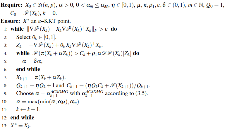
Lemma 1 guarantees that we will be able to decrease the value of the objective function through-out the iterations. In addition, note that if we select θ_k =1 then the update scheme (3.1)-(3.3) reduces to the Riemannian steepest descent method (RSD) proposed by Manton in¹³, while if we choose θ_k =0 then we recover the spectral gradient projection method (SPG), (see equation (2.5) in¹⁰). Therefore, the convex combination (3.3) constitutes a unified framework that incorporates the SPG and RSD methods in the extreme values of the parameter θ_k , while the intermediate values θ_k ∈(0, 1) correspond to new non-Riemannian gradient type methods. In general, the approach (3.1)-(3.3) defines a non-countable family of effective projected gradiente-type methods for the solution of problem (1.1).

Example 3.1.Now we present an example to illustrate the numerical behavior of our update scheme by considering θ_k=θ constant along the iterations but using several values of θ. In this example, the WOPP problems are generated by the following Matlab commands: randn(′seed′, 5); A=diag(diag(ones(m)/sqrt(n))); B=rand(m, n)/sqrt(m); C=eye(n); and [X₀, ~]=qr(randn(m, n), 0). In addition, we set m=100, n=10 and ε=1e-5. We solve this toy experiment with our porposed iterative scheme given by(3.1)-(3.3), for θ∈{0, 0.25, 0.5, 0.75, 1}. The convergence behavior of the logarithm of the gradient norm log(||∇ℱ(X)|| _F ) along the iteration is presented inFigure 1. In this figure, we note that the performance of theAlgorithm 1changes for different values of θ.

Algorithm 1
Gradient projection method

Figure 1
Behavior of the Algorithm 1 varying θ. The y-axis represents the logarithm of the gradient norm, that is log(||∇ℱ(X _k )-X _k ∇ℱ(X _k )^⊤ X _k ||_F )

On the other hand, we have not yet explained how we determine the scalar α_k >0 in our developed projected line-search procedure (3.1)-(3.3). In practice, we employ a non-monotone globalization strategy combined with an adaptive Barzilai-Borwein step-size. It is well-known that the Barzilai-Borwein^{2), (19} step-sizes (BB-steps) can greatly speed up the convergence of the gradient-type methods, without increasing the computational cost too much. In view of these numerical advantages, we use the recently published cyclic delayed weighted steplength¹⁷.

${\alpha }_k^{ACSDMG}=\left\{\begin{array}{ll}min\left\{{\alpha }_i^{CSDMG}:i\in {\mathcal{I}}_k^m\right\}& if{\alpha }_k^{CSDMG}<\kappa {\alpha }_k^{BB1}\\ {\alpha }_k^{CSDMG}& otherwise,\end{array}\right.$ (3.5)

where ${\mathcal{I}}_k^m=\left\{max\left\{1,...,k-m\right\},...,k\right\}$, m∈ℕ, κ∈(0, 1) and ${\alpha }_k^{CSDMG}$ is given by

${\alpha }_k^{CSDMG}={\alpha }_k^{BB2}\left(\frac{\left(1-\mu \right){\alpha }_k^{BB1}+2\mu }{\left(1-\mu \right){\alpha }_k^{BB2}+2\mu }\right).$ (3.6)

where µ∈[0, 1] is a fixed value. In addition, in (3.6) the parameters ${\alpha }_k^{BB1}$ and ${\alpha }_k^{BB2}$ refer to the classical Brazilai-Borwein step-sizes², i.e.

${\alpha }_k^{BB1}=\frac{{||S_{k-1}||}_F^2}{\left|tr\left[S_{k-1}^{\top }{Y}_{k-1}\right]\right|}and{\alpha }_k^{BB2}=\frac{\left|tr\left[S_{k-1}^{\top }{Y}_{k-1}\right]\right|}{{||Y_{k-1}||}_F^2},$ (3.7)

where S _k-1 =X _k -X _k-1 and Y _k-1 =∇ℱ(X _k )-∇ℱ(X _k-1 ). Because the inner product $tr\left[S_{k-1}^{\top }{Y}_{k-1}\right]$ can be equal to zero (or very close to zero); or it can even be very large, we will consider the following safeguard to avoid numerical errors

${\hat{\alpha }}_k^{ACSDMG}=max\left\{min\left\{{\alpha }_k^{ACSDMG},{\alpha }_M\right\},{\alpha }_m\right\},$

where 0<α_m ≤α_M <1e16 are two global parameters chosen by the user. In addition, since the BB-type step-sizes do not necessary guarantee descent of the cost function along the iterative process, these step-sizes are generally used in combination with some globalization technique in order to ensure the global convergence. For this end, we use the non-monotone globalization technique proposed by Zhang and Hager in²⁶. The above description leads us to Algorithm 1.

It follows from Lemma 1 and Proposition 3 that the sequence of search directions {Z _k } generated by Algorithm 1 is a sequence of gradient-related directions (see Definition 4.2.1 in¹), hence if we set η=0 (in this case the Zhang-Hager condition is reduced to the Armijo rule¹²) then we can repeat the steps of the proof of Theorem 4.3.1 and Corollary 4.3.2 that appear in¹ to obtain the global convergence of our proposal. Similarly, to derive the global convergence of Algorithm 1 for the case η∈(0, 1), we can replicate the steps of the proofs of Lemma 2 and Theorem 1 that appear in¹⁴.

Now let us consider the particular case of (1.1) when C=I _n is the n-by-n identity matrix and A∈ℝ^m×m is a square matrix, that is, let us consider the following problem

$\underset{X\in {\mathrm{ℝ}}^{m\times n}}{min}\frac{1}{2}{||AX-B||}_F^2,subjectto{X}^{\top }X=I,$ (3.8)

where B is a known real matrix of correct dimensions. This problems is known as “unbalanced orthogonal procrustes problem” (OPP)^{23), (27), (28}. In general, this problem does not have an analytical solution, except in the case when m=n, see^{21), (23), (28}. However, if A is positive definite matrix then we can derive a problem similar to (3.8) with closed-form solution.

Lemma 2.Let A∈ℝ ^m×m be a positive definite matrix, B∈ℝ ^m×n . Let us consider the the non-convex constrained optimization problem

$\underset{X\in {\mathrm{ℝ}}^{m\times n}}{min}\frac{1}{2}{||AX-B||}_{A^{-1}}^2,subjectto{X}^{\top }X=I,$ (3.9)

where${||P||}_{A^{-1}}:=\sqrt{tr\left(P^{\top }{\left(A{A}^{\top }\right)}^{-1}P\right)}={||A^{-1}P||}_F$, for any P∈ℝ ^m×n . Then, the global solution of(3.9)is$\hat{X}=\pi \left(A^{-1}B\right)=U{I}_{m,n}{V}^{\top }$, where A ^-1 B=UΣV ^⊤ represents the singular value decomposition of A ^-1 B.

Proof. Let $H\left(X\right)=\frac{1}{2}{||AX-B||}_{A^{-1}}^2$ be the cost function of (3.9). Notice that

$H\left(X\right)=\begin{array}{c}\frac{1}{2}tr\left[{\left(AX-B\right)}^{\top }{\left(A{A}^{\top }\right)}^{-1}\left(AX-B\right)\right]\\ \frac{1}{2}tr\left[{\left(AX-B\right)}^{\top }{A}^{-\top }{A}^{-1}\left(AX-B\right)\right]\\ \frac{1}{2}tr\left[\left(X^{\top }-B^{\top }{A}^{-\top }\right)\left(X-A^{-1}B\right)\right]\\ \frac{1}{2}tr\left[{\left(X-A^{-1}B\right)}^{\top }\left(X-A^{-1}B\right)\right]\\ \frac{1}{2}{||X-A^{-1}B||}_F^2.\end{array}$ (3.10)

So, the optimization problem (3.9) is equivalent to

$\underset{X\in St\left(m,n\right)}{min}{||X-A^{-1}B||}_F^2.$

Thus, by applying Proposition 1, we have that the global minimizer of (3.9) is $\hat{X}=\pi \left(A^{-1}B\right)$, completing the proof. □

It follows from the lemma above that if we replace the Frobenius norm in (3.8) by the ${||·||}_{A^{-1}}$ then the new procrustes problem has an analytical solution. This result can be used to initialize Algorithm 1 with the point X ₀=π(A ^-1 B), for the case when A is positive definite and C is the identity matrix.

4 COMPUTATIONAL EXPERIMENTS

In order to give further insight into the Algorithm 1, we present some numerical comparisons. For benchmarking, we compare our method with the Riemannian gradient method based on the Cayley transform OptSt developed in^{25 1}, the Riemannian steepest descent method (Manton-SD) introduced by Manton in¹³, and the Riemannian conjugate gradient methods Algor.1a and Algor.1b proposed in^{29 2}. All the experiments have been performed on a intel(R) CORE(TM) i7-4770, CPU 2.20 GHz with 1TB HD and 16GB RAM. The algorithm was coded in Matlab (version 2017b).

In this section, Time, Nfe, Nitr and Grad will denote the averaged total computing time in seconds, the average number of function evaluations, the average number of iterations, the averaged residual ||∇ℱ(X*)||_F where X* is the optimum estimated by each method, respectively. In addition, we stop the methods if one of the following conditions holds: (i) k≥N; (ii) ||∇ℱ(X _k )-X _k ∇ℱ(X _k )^⊤ X _k ||_F ≤ε, where the values of N and ε will be specificated for each experiment. In our Algorithm 1, we set α_m =1e-15, α_M =1e+15, ρ₁=1e-4, η=0.85, δ=0.2, (m, κ)=(9, 0.8) and µ≡µk=(k+1)/(k+2) varying along the iterations.

For the first experiment, we consider the following optimization problem

$\underset{x\in {\mathrm{ℝ}}^n}{min}{x}^{\top }Lx,s.t.x^{\top }x=1,$ (4.1)

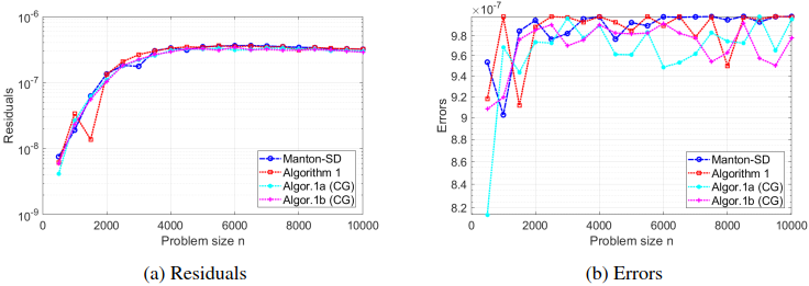
where L∈ℝ^n×n is a symmetric matrix. Problem (4.1) can be seen as a particular version of problem (1.1) obtained by substituting C=1 and B=(0, 0, ..., 0)^⊤ in (1.1); and considering the identification L=A ^⊤ A. It is well-known that the global solution of (4.1) corresponds to the eigenvector associated with the smallest eigenvalue of L. In fact, problem (4.1) is equivalent to minimizing the Rayleigh quotient of L. For this experiment, we solve (4.1) for the following 20 values of n, n∈{500, 1000, 1500, ..., 9500, 10000}. In order to make this experiment replicable, we construct the matrix L as the discrete Laplacian operator, generated with the following Matlab command L=gallery(‘tridiag’, n, -1, 2, -1), and the initial vector x ₀∈ℝⁿ is chosen as x ₀=v/||v||₂, where v=(1, 2, 3, ..., n)^⊤. In this computational study, we use N=15000, choose ε=1e-6; and θ_k =k/(k+1) in our algorithm. The accuracy of the computed eigenvalue and its associated eigenvector of L are measured by using the absolute error

$error={||L\hat{x}-\left({\hat{x}}^{\top }L\hat{x}\right)\hat{x}||}_2,$

and the absolute residual in the objective value

$residual=\left|f\left(\hat{x}\right)-{\lambda }_{min}\right|,$

where $\hat{x}$ denote the estimated solution of (4.1) obtained by each method, and λ_min is the smallest eigenvalue of L.

Table 1 summarizes the average values Time, Nfe, Nitr and Grad obtained by every method. As shown in Table 1, the most efficient methods in terms of computational time and number of iterations are Algorithm 1 and the Riemannian gradient method proposed by Manton in¹³. In Figure 2, we show the absolute error and the absolute residual for each method and for each value of n. From Figure 2, we can see that all the methods obtain the global solution of problem (4.1), for all the considered values of n, with the pre-established precision. Furthermore, we observe that Algorithm 1 converges to the solution faster than the Riemannian conjugate gradient methods Algor.1a and Algor.1b.

Figure 2
The residuals of the computed eigenvalues (a) and the corresponding absolute errors (b), of a tridiagonal matrix. The y-axis is in logarithmic scale.

Table 1
Numerical results computing the smallest eigenvalue of tridiagonal matrices.

Method	Nitr	Nfe	Time	Grad
Manton-SD	3790.1	3894.2	0.51	9.87e-7
Algor.1a (CG)	12821.0	12854.0	3.16	9.65e-7
Algor.1b (CG)	12971.0	12971.0	3.12	9.71e-7
Algorithm 1	3530.7	3634.2	0.37	9.85e-7

Our second experiment was taken from²⁰. Let n=q, p=m, A=PSR ^⊤ and C=QΛQ ^⊤, where P, Q and R are orthogonal matrices randomly generated such that Q∈ℝ^n×n , R, P∈ℝ^m×m , Λ∈ℝ^n×n is a diagonal matrix with entries generated from a uniform distribution in the range $\left[\frac{1}{2},2\right]$ and S is a diagonal matrix defined for each type of problem, see below for details. When not specified, the entries of the matrix were generated using the standard Gaussian distribution. The matrix B was randomly generated with entries follow a normal standard distribution. Finally, for the different tested problems the diagonal matrix S is described below.

Structure 1: The diagonal elements of S were generated by a normal distribution in the interval^{10), (12}.

Structure 2: The diagonal of S is given by S _ii =i+2r _i , where r _i was a random number uniformly distributed in the interval [0, 1].

Structure 3: Each diagonal element of S was generated as follows: $S_{ii}=1+\frac{99\left(i-1\right)}{m+1}+2r_i$, with r _i uniformly distributed in the interval [0, 1].

In this experiment, we use N=50000 and choose ε=1e-6; and θ_k =1/(k+9) for our algorithm. For all experiments, we randomly generate the starting point X ₀ using the following Matlab command [X ₀, ~]=qr(randn(n, p), 0). In all the experiments, we solve 10 independent instances for the different values of (n, p) and then we report the average values Time, Nfe, Nitr and Grad. The numerical results concerning this test are contained in Table 2. From Table 2, we can see that all the methods obtain an approximated solution with the required precision. In addition, we note that our procedure obtains competitive results compared to the existing methods in the literature. Finally, we notice that the most efficient methods, in terms of computational time, were the OptSt method and our Algorithm 1.

Table 2
Numerical results on weighted orthogonal procrustes problems.

Method	Nitr	Nfe	Time	Grad	Nitr	Nfe	Time	Grad
	Structure 1 with n=500 and p=70				Structure 1 with n=1000 and p=100
OptSt	37.4	38.4	0.12	6.40e-6	37.0	39.0	0.35	5.68e-6
Algor.1a (CG)	43.6	46.6	0.17	7.16e-7	40.9	43.1	0.53	6.97e-7
Algor.1b (CG)	34.0	36.0	0.12	6.90e-7	44.7	47.4	0.56	8.14e-7
Algorithm 1	31.2	34.2	0.07	6.58e-6	34.2	35.2	0.31	6.23e-6
	Structure 2 with n=100 and p=50				Structure 2 with n=100 and p=100
OptSt	2942.5	3112.0	1.87	1.94e-6	2290.7	2494.0	1.96	8.41e-6
Algor.1a (CG)	4640.5	7735.2	6.00	1.07e-3	3033.5	4870.1	9.94	7.85e-7
Algor.1b (CG)	4488.8	7453.7	5.00	1.48e-4	3440.5	5607.5	8.97	8.49e-7
Algorithm 1	2293.8	2434.0	1.11	9.24e-6	2275.6	2377.1	2.51	9.55e-6
	Structure 3 with n=300 and p=20				Structure 3 with n=1000 and p=100
OptSt	3397.2	3556.5	1.78	9.10e-6	957.4	999.5	2.56	8.42e-6
Algor.1a (CG)	6741.9	11863.0	5.93	2.55e-4	1136.5	1869.5	3.32	9.12e-7
Algor.1b (CG)	7289.0	12784.0	5.92	1.13e-3	1134.2	1876.3	3.35	8.61e-7
Algorithm 1	2865.8	3010.5	0.97	8.93e-6	751.4	789.7	1.41	9.21e-6

5 CONCLUDING REMARKS

In the present work, we have proposed a novel feasible line-search algorithm for solving a class of linear least-square optimization problems on the Stiefel manifold. In particular, we have introduced a projected gradient-type method with mixed direction, which uses the non-monotone globalization strategy of Zhang and Hager combine with an alternate Barzilai-Borwein step-size. All operations are performed with matrices to preserve the structure of the problem and avoiding vectorization. The search direction used by our method involves the Riemannian gradient in order to exploit the geometric information of the Stiefel manifold. In addition, the search directions computed by our algorithm were proved to satisfy the sufficient descent condition, which guarantees that the method reduces the value of the cost function throughout the iterative process. A numerical study with problems taken from the literature shows the reliability of adopting this new approach for solving weighted orthogonal procrustes problems.

Our numerical results show that the new family of methods works very well for any selection of the parameter θ in the interval [0, 1]. But, since θ may be a problem dependent parameter, then it will remain as future work, to develop and investigate self-adaptive strategies to select this parameter along the iterative process, possibly using local information of the objective function, in order to improve the performance of the new collection of methods.

REFERENCES

• ¹ P.A. Absil, R. Mahony & R. Sepulchre. “Optimization algorithms on matrix manifolds”. Princeton University Press (2008).
• ² J. Barzilai & J.M. Borwein. Two-point step size gradient methods. IMA journal of numerical analysis, 8(1) (1988), 141-148.
• ³ T. Bell. Global positioning system-based attitude determination and the orthogonal procrustes problem. Journal of guidance, control, and dynamics, 26(5) (2003), 820-822.
• ⁴ E.G. Birgin, J.M. Martínez & M. Raydan. Nonmonotone spectral projected gradient methods on convex sets. SIAM Journal on Optimization, 10(4) (2000), 1196-1211.
• ⁵ E.G. Birgin, J.M. Martínez & M. Raydan. Spectral projected gradient methods: review and perspectives. Journal of Statistical Software, 60 (2014), 1-21.
• ⁶ A. Edelman, T.A. Arias & S.T. Smith. The geometry of algorithms with orthogonality constraints. SIAM journal on Matrix Analysis and Applications, 20(2) (1998), 303-353.
• ⁷ X. Feng, W. Yu & Y. Li. Faster matrix completion using randomized SVD. In “2018 IEEE 30th International conference on tools with artificial intelligence (ICTAI)”. IEEE (2018), p. 608-615.
• ⁸ J. Francisco, F.V. Bazán & M.W. Mendonça. Non-monotone algorithm for minimization on arbitrary domains with applications to large-scale orthogonal procrustes problem. Applied Numerical Mathematics, 112 (2017), 51-64.
• ⁹ J.R. Hurley & R.B. Cattell. The Procrustes program: Producing direct rotation to test a hypothesized factor structure. Behavioral science, 7(2) (1962), 258.
• ¹⁰ B. Jiang & Y.H. Dai. A framework of constraint preserving update schemes for optimization on Stiefel manifold. Mathematical Programming, 153(2) (2015), 535-575.
• ¹¹ E. Kokiopoulou, J. Chen & Y. Saad. Trace optimization and eigenproblems in dimension reduction methods. Numerical Linear Algebra with Applications, 18(3) (2011), 565-602.
• ¹² D.G. Luenberger, Y. Ye, et al. “Linear and nonlinear programming”, volume 2. Springer (1984).
• ¹³ J.H. Manton. Optimization algorithms exploiting unitary constraints. IEEE transactions on signal processing, 50(3) (2002), 635-650.
• ¹⁴ H. Oviedo. Global convergence of Riemannian line search methods with a Zhang-Hager-type condition. Numerical Algorithms, 91(3) (2022), 1183-1203.
• ¹⁵ H. Oviedo. Implicit steepest descent algorithm for optimization with orthogonality constraints. Optimization Letters, 16(6) (2022), 1773-1797.
• ¹⁶ H. Oviedo. Proximal point algorithm with Euclidean distance on the Stiefel manifold. Mathematics, 11(11) (2023), 2414.
• ¹⁷ H. Oviedo. A cyclic delayed weighted steplength for the gradient method. Ricerche di Matematica, 73(2) (2024), 873-885.
• ¹⁸ H. Oviedo, O. Dalmau & R. Herrera. Two novel gradient methods with optimal step sizes. J. Comput. Math., 39(3) (2021), 375-391.
• ¹⁹ H. Oviedo, O. Dalmau & H. Lara. Two adaptive scaled gradient projection methods for Stiefel manifold constrained optimization. Numerical Algorithms, 87 (2021), 1107-1127.
• ²⁰ H. Oviedo, H. Lara & O. Dalmau. A non-monotone linear search algorithm with mixed direction on Stiefel manifold. Optimization Methods and Software, 34(2) (2019), 437-457.
• ²¹ P.H. Schönemann. A generalized solution of the orthogonal procrustes problem. Psychometrika, 31(1) (1966), 1-10.
• ²² I. Söderkvist & P.A. Wedin. On condition numbers and algorithms for determining a rigid body movement. BIT Numerical Mathematics, 34 (1994), 424-436.
• ²³ T. Viklands. “Algorithms for the weighted orthogonal procrustes problem and other least squares problems”. Ph.D. thesis, Datavetenskap (2006).
• ²⁴ Z. Wen, C. Yang, X. Liu & Y. Zhang. Trace-penalty minimization for large-scale eigenspace computation. Journal of Scientific Computing, 66 (2016), 1175-1203.
• ²⁵ Z. Wen & W. Yin. A feasible method for optimization with orthogonality constraints. Mathematical Programming, 142(1) (2013), 397-434.
• ²⁶ H. Zhang & W.W. Hager. A nonmonotone line search technique and its application to unconstrained optimization. SIAM Journal on Optimization, 14(4) (2004), 1043-1056.
• ²⁷ L. H. Zhang, W.H. Yang, C. Shen & J. Ying. An eigenvalue-based method for the unbalanced Procrustes problem. SIAM journal on Matrix Analysis and Applications, 41(3) (2020), 957-983.
• ²⁸ Z. Zhang, Y. Qiu & K. Du. Conditions for optimal solutions of unbalanced Procrustes problem on Stiefel manifold. Journal of Computational Mathematics, (2007), 661-671.
• ²⁹ X. Zhu. A Riemannian conjugate gradient method for optimization on the Stiefel manifold. Computational optimization and Applications, 67 (2017), 73-110.

¹

The OptSt Matlab code is available in https://github.com/wenstone/OptM

²

The Riemannian conjugate gradient methods Algor.1a, Algor.1b and Algor.1b+ZH can be downloaded from http://www.optimization-online.org/DB_HTML/2016/09/5617.html

*

Corresponding author: Harry Fernando Oviedo Leon - E-mail: [e-mail]

Publication Dates

• Publication in this collection
  22 Nov 2024
• Date of issue
  2024

History

• Received
  06 Nov 2023
• Accepted
  03 May 2024