Temporal and Spatial Uncertainty of Erosion Soil Loss from an Argisol Under Sugarcane Management Scenarios

ABSTRACT

The identification of erosion-susceptible areas is fundamental for the adoption of soil conservation practices. Thus, the best way to estimate the spatial pattern of soil erosion must be identified, in which the process uncertainties are also taken into consideration. The purpose of this study was to evaluate the spatial and temporal uncertainty of soil loss under two scenarios of sugarcane harvest management: green cane (GC) and burnt cane (BC). The study was carried out on a 200-ha area, in Tabapuã, São Paulo State, Brazil. A regular 626-point sampling grid was established in the area, with equidistant intervals of 50 m and a final plant density of about 3.3 samples per ha. The probability that the soil loss would exceed the tolerable limit of 6.67 t ha^-1 yr^-1 was estimated for each management scenario and after the five harvests. The temporal uncertainty was determined by integrating the estimated annual probabilities, representing the harvests. Areas with soil loss risks above the threshold were identified based on probability maps, generated from the individual and combined dichotomous variables. Soil losses from the BC were highest, during all five harvests. With the exception of the 5^th harvest and the entire cultivation cycle under GC, all soil loss estimates were spatially dependent. From the 4^th harvest under GC, the probability of the soil loss exceeding the threshold was above 80 % in zero percent of the area, whereas, for BC, the probability exceeded 80 % in 40 % of the area. The production cycle allowed the delimitation of priority areas for the adoption of conservation practices in each management. In the BC, areas with steeper slopes were more likely to exceed the threshold with lower uncertainties.

Keywords
green cane; burnt cane; geostatistics; indicator kriging

INTRODUCTION

Brazil is the world's largest sugarcane (Saccharum spp.) producer and within the country, it is the second most cultivated crop, only after soybean. The sugarcane production for the 2017/18 growing season is estimated at 647.6 million tons. Currently, an area of 8,838.5 thousand hectares is growing sugarcane, distributed in all producing states, of which São Paulo has the largest output, accounting for 51.6 % of the total production, grown on 4,558.4 thousand hectares (Conab, 2017).

In view of the expansion of the sugar and ethanol industry, changes in the sugarcane management system may have a significant impact on the Brazilian production, since the form of sugarcane harvesting can influence crop yield and longevity, the physical, chemical and biological properties, and the environment (Souza et al., 2006).

Controlled burning of cane fields prior to manual harvesting is still a common practice in several sugarcane regions of Brazil, with the objective of reducing the amount of cane straw, thus facilitating the cutting and mechanical loading operations. This practice, from the point of view of soil and water conservation, has been a matter of concern and the focus of a number of studies, for tending to increased nutrient losses due to erosion (Martins Filho et al., 2009; Silva et al., 2012; Sousa et al., 2012). On the other hand, under the green cane management, a layer of residual plant material is left on the soil surface after mechanical harvesting, contributing to enhance the structure and increase the cation exchange capacity of the soil (Oliveira et al., 1999), and to increase resistance to the physical degradation caused by machine traffic in the area (Garbiate et al., 2011).

The conversion of burnt cane to mechanical harvesting (GC) system becomes as important as agricultural expansion of the sugarcane crop itself. Consequently, several studies addressed an evaluation of the spatial variability of soil loss, as well as erosion factors in areas under sugarcane cultivation (Weill and Sparovek, 2008; Sanchez et al., 2009; Andrade et al., 2011; Garbiate et al., 2011).

Aside from degradation due to soil losses, erosion processes carry nutrients and pollutants into water bodies and ecosystems close to eroding sites, either bound to soil particles or as soluble material in surface runoff water (Neves et al., 2015; Comino et al., 2016). The soil degradation processes are interlinked with edaphic, climatic, and anthropogenic factors. The intensity and development rate of these processes are fueled by inadequate land use and management, exposing the soil to weathering factors that induce the gradual destruction of its physical, chemical, and biological properties (Laufer et al., 2016).

Spatial and temporal variability of erosion processes in Brazilian soils is great due to the diversity of the climate, influencing the erosive potential of rains, and of the edaphic diversity, with soils tending to be erosion-susceptible (Neves et al., 2015). This is particularly true for the more erosion-susceptible Argisols, due to their pedogenesis and intrinsic factors, as well as to the commonly applied management systems (Bertol et al., 2002). Thus, the estimation of soil erosion and generation of scenarios by modeling with geostatistical techniques are therefore useful in the prevention of soil and nutrient losses, to compile important information to assist environmental management and land use planning (Galharte et al., 2014).

Geostatistical methods such as ordinary kriging (OK) and indicator kriging (IK) provide estimates of values in non-sampled regions of the study area. Although these methods produce interpolated values, they have different objectives and results. Ordinary kriging (OK) provides unbiased estimates of a variable with minimum variance at non-sampled locations (Goovaerts, 1997). In addition, OK is a point predictor, used to predict spatial averages. Indicator kriging, on the other hand, evaluates the probabilities of occurrence of events, e.g. exceeding a threshold.

In this paper, the term “uncertainty” was defined as proposed in a study of Mowrer (2000), in which the author coined this term for situations in which the exact value of the error of an estimate is unknown. Aside from constructing spatial distribution maps, the spatial uncertainty of these estimates must be assessed, thus providing a precision parameter of the generated spatial information (Mondal et al., 2017).

Indicator kriging has been successfully used because it allows expressing the spatial model in terms of probability of excess (Silva et al., 2009). Instead of presenting the interpolation results in terms of classes of fixed values, they can be presented in terms of the probability that a given threshold is exceeded or, if desired, unreached (Goovaerts, 1997).

The IK method allows the identification of areas with region-specific management, meeting the premises of precision agriculture, and can contribute to increase crop yields, optimize the use of agricultural inputs, reduce expenses with applications, and allow an efficient control of the environmental impact of agriculture (Motomiya et al., 2006). The objective of this study was to evaluate the spatial and temporal uncertainty of soil loss under two sugarcane management scenarios, i.e., green and burnt cane cultivation, on an Argisol.

MATERIALS AND METHODS

Study area

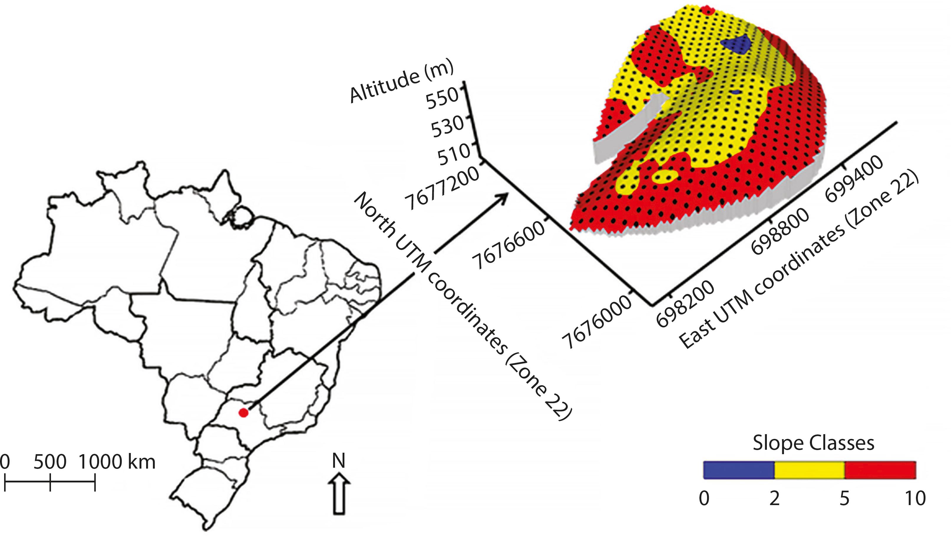
The experimental area (21° 05′ S; 49° 01′ W) is located in the district of Tabapuã, in the northwest of São Paulo State, Brazil (Figure 1). The 200-ha area had been intensively cultivated with sugarcane for the previous 20 years. The regional climate, according to the Thornthwaite classification system, is metamorphic (C₂dA′a′), rainy subhumid, with little or no water surplus, and summer evapotranspiration below 48 % of the annual total. The annual average precipitation is 1,318 mm and rainfalls are concentrated in the period from November to February.

Figure 1
Location of the experimental area, slope class, and distribution of sampling points (•).

The region is located in the geomorphic province of the highland in the west of São Paulo State (Planalto Ocidental Paulista). The parent material consists of geological units of sedimentary arenitic rocks of the Bauru Group, Adamantina mountain range (IPT, 1981). It is characterized by fine-grained to very fine sandstone banks, with the occurrence of clay and cement pebbles and carbonate nodules.

According to Santos et al. (2013a), the soil was classified as medium/clay texture Argissolo Vermelho-Amarelo Eutrófico [Alfisol (Soil Survey Staff, 2014)]. The primary vegetation of the region was classified as seasonal rainforest and Cerrado (tropical savannah). For the geomorphological and pedological characterization, we used 1:35,000 aerial photographs, field evaluations, and altimetric profile analysis. The slope map was obtained from the digital elevation model, based on slope intervals, as defined by Lepsch (1991): (a) - plane (0-2 %); (b) - gently undulating (2-5 %); (c) - moderately undulating (5-10 %).

Sample grid and sugarcane management scenarios

To estimate the soil loss, the databank of soil physical and chemical properties of the surface layer (0.00-0.20 m) established by Sanchez et al. (2009) was used. The soil was sampled at the grid cross points, at regular intervals of 50 m, resulting in a total of 626 geo-referenced points or a sample density of 3.3 samples per ha, considered a detailed survey scale, according to Santos et al. (1995). Two sugarcane management scenarios were considered: (i) green cane (GC), characterized mainly by mechanical harvesting without burning and crop residues left on the soil surface; and (ii) burnt cane (BC), mainly characterized by the burning of crop residues prior to manual harvesting.

In the two studied managements, the production cycles (1^st to 5^th harvests) and sugarcane variety (SP-813250) were the same and similar cultural treatments were applied. For the 1^st harvest, in both managements, soil tillage for the installation of the crop was the same and was followed by the same cultural treatments until the first sampling, after harvest. Therefore, the soil loss of the 1^st harvest was considered as the experimental control, since the factors soil cover and management and conservation practices did not vary according to the management.

Estimation of soil loss

Soil erosion losses in both managements were estimated based on soil physical and chemical properties measured by Sanchez et al. (2009), and on results of erosion factors determined by Martins Filho et al. (2009) and Andrade et al. (2011), according to the Universal Soil Loss Equation (USLE) (Wischmeier and Smith, 1978) (Equation 1):

Eq. 1 $$\text{A}=\text{R}\times \text{K}\times \text{LS}\times \text{C}\times \text{P}$$

in which, A = soil loss per unit area (t ha^-1 yr^-1); R = rainfall erosivity factor (MJ mm ha^-1 h^-1 yr^-1); K = soil erodibility factor (t h MJ^-1 mm^-1); LS = factor of the combined effect of slope and slope length; C = soil cover and management factor; and P = factor conservation practices.

At each sampling grid point (Figure 1), the values of erosivity (R); erodibility (K); combined slope and slope length effect (LS); soil cover and management (C); and conservation practices were determined. However, the factors erosivity (R) and soil cover and management (C) varied according to the harvest.

The erosivity of the local rains (R) was estimated based on the method proposed by Lombardi Neto et al. (2000). The erodibility factor (K) was estimated locally by artificial rain simulation, as described by Martins Filho (2007), and compared with the method proposed by Denardin (1990). The LS factor was determined as suggested by Wischmeier and Smith (1978). For factor P, the values proposed by Bertoni and Lombardi Neto (1990) were adopted.

The values used for factor C were established as described by Andrade et al. (2011): (1) burnt cane - 0.16 (1^st harvest); 0.13 (2^nd harvest); 0.16 (3^rd harvest); 0.13 (4^th harvest); 0.13 (5^th harvest); and (2) green cane - 0.16 (1^st harvest); 0.10 (2^nd harvest); 0.09 (3^rd harvest); 0.07 (4^th harvest); 0.06 (5^th harvest).

Although there are more precise models than the USLE, we decided to use it in the original form in this study. The reason was that the experimental work carried out in the area established the underlying factors (R, K, LS, C, and P) with high certainty. Due to the uncertainties resulting from this adoption, it was not possible to evaluate the impacts of liquid erosion and sediment deposition along slopes. Only the spatial and temporal uncertainties of the sediment production potential in the area could be evaluated by the USLE.

The annual mean values of rainfall erosivity (R = ΣEI₃₀) were calculated by equation 2, using software NetErosividade SP (Moreira et al., 2006):

Eq. 2 $${\text{EI}}_{\text{30i}}=89.823{\left(\frac{{\text{Pm}}^2}{\text{Pa}}\right)}^{0.759}$$

in which EI_30i (MJ mm ha^-1 h^-1) = mean monthly erosivity; i = 1 to 12; Pm = mean monthly precipitation in month i (mm); and Pa = mean annual precipitation (mm).

From the values of EI_30i, the fractions of the annual erosivity index (FEI_30i) were calculated, for each of the five harvests of the entire sugarcane crop cycle (Table 1). The FEI_30i were used to calculate factor C.

Table 1
Fraction of rainfall erosivity (FEI₃₀) in sugarcane development stages in Tabapuã - SP

Stages	1st harvest (2002-2003)	2nd harvest (2003-2004)	3rd harvest (2004-2005)	4th harvest (2005-2006)	5th harvest (2006-2007)
	----------------------------------------------------------------- MJ mm ha-1 h-1 -----------------------------------------------------------------
1	0.446	0.268	0.430	0.336	0.385
2	0.000	0.032	0.037	0.017	0.004
3	0.010	0.018	0.066	0.017	0.049
4	0.173	0.213	0.178	0.257	0.125
5	0.365	0.451	0.281	0.364	0.388
6	0.006	0.019	0.007	0.009	0.049

• 1: soil tillage until planting (January-March); 2: planting until one month after tillage (April); 3: crop establishment (May-June); 4 and 5: crop growth (July-December) and maturation (January-April); 6: harvest (May-June).

The erodibility (K) was estimated point by point by the equation 3, proposed by Denardin (1990):

Eq. 3 $$\text{K}=\text{0.00000748 M + 0.004448059 p - 0.06631175 MWD}+\text{0.01039567 X32}$$

in which: M = new silt (new silt + new sand); p = permeability encoded according to Wischmeier et al. (1971); MWD = mean weight diameter of soil particles smaller than 2.00 mm; X32 = new sand (MO/100); new silt = silt + very fine sand (%); new sand = very coarse sand + coarse sand + medium sand + fine sand (%); MO = organic matter (%).

The mean value of the estimated factor K was 0.024 Mg ha^-1 MJ^-1 mm^-1 ha h, which did not differ significantly by the t test from that determined by Amaral (2003) at 0.023 Mg ha^-1 MJ^-1 mm^-1 ha h, in an experimental plot, with the same Argisol as in this study.

The factor LS was determined using equation 4, proposed by Wischmeier and Smith (1978):

Eq. 4 $$\text{LS}={(\text{λ}/22.13)}^{\text{m}}(65.41\text{sen}2\text{θ +}4.56\text{senθ + 0.065)}$$

in which λ = slope length (m); m = variable exponent with terrain slope; and θ = slope angle in degrees.

The values of soil loss ratios (SLR) used to calculate factor C for each harvest are presented in table 2. The factor C for each harvest during the entire crop cycle was calculated as the product of SLR and FEI₃₀ of the above stage (Table 1).

Table 2
Ratios of soil loss (SLR) by erosion in sugarcane development stages, under burnt cane (BC) and green cane (GC) management systems, from the 1^st to the 5^th harvest

Stages	1st to 5th Harvest (BC)	1st Harvest (GC)	2nd Harvest (GC)	3rd Harvest (GC)	4th Harvest (GC)	5th Harvest (GC)
1	0.27	0.27	0.14	0.11	0.10	0.07
2	0.22	0.22	0.12	0.08	0.08	0.06
3	0.11	0.11	0.11	0.08	0.04	0.06
4	0.03	0.03	0.09	0.07	0.06	0.06
5	0.08	0.08	0.07	0.07	0.06	0.06
6	0.18	0.18	0.06	0.06	0.06	0.06

• 1: soil tillage until planting (January-March); 2: planting until one month after tillage (April); 3: crop establishment (May-June); 4 and 5: crop growth (July-December) and maturation (January-April); 6: harvest (May-June).

The sum of the SLR × FEI₃₀ of the stages of the crop cycle were used to compute factor C related to the sugarcane harvests, according to Andrade et al. (2011). The following values were estimated for factor C: (1) burnt sugarcane - 0.16 (1^st harvest); 0.13 (2^nd harvest); 0.16 (3^rd harvest); 0.13 (4^th harvest); 0.13 (5^th harvest); and (2) green cane - 0.16 (1^st harvest); 0.10 (2^nd harvest); 0.09 (3^rd harvest); 0.07 (4^th harvest); 0.06 (5^th harvest).

For factor P, values proposed by Wischmeier and Smith (1978) were adopted, due to the slope of the terrain. The tolerance to erosion soil loss (T) was determined at 6.67 Mg ha^-1 yr^-1, based on soil properties, according to the method proposed by Oliveira et al. (2008).

Statistical and geostatistical analysis

Initially, soil erosion variability was evaluated by descriptive statistics, calculating the mean, standard deviation, 1^st and 3^rd quartiles, and minimum and maximum values. Subsequently, the data were subjected to geostatistical analysis by means of variogram modeling and interpolation by indicator kriging.

The characterization of the spatial distribution of values above or below a cut-off value Z_k requires a priori coding of each observation Z(x_i), for values above the established cut-off level Z_k, at one (1), and those below, at zero (0) (Equation 5):

Eq. 5 $$I(x_i;z_k)=\{\begin{array}{c}z(x_i)\ge z_k\\ 0\mathrm{otherwise}\end{array}$$

Thus, by adopting a cut-off value Z_k for which soil loss may not exceed the threshold, the random variable Z(x_i) is converted into an indicator function, for which value 1 means the occurrence of loss of soil above the acceptable limit, and value 0 the non-occurrence of soil loss above this limit (Goovaerts, 1997). This cut-off value was established based on the soil loss tolerance of an Argisol (Oliveira et al., 2008), defined as 6.67 t ha^-1 yr^-1.

The temporal analysis (production cycles) was performed, considering all dichotomized values for each harvest and of both managements. Thus, values of 1 were assumed for locations where, for all harvests, the values exceeded the soil loss tolerance limit. Thus, the production cycles represent the combined probability of the separate harvests that the soil losses would exceed the established threshold.

Prior to interpolation by indicator kriging, the variogram must be modeled. The indicator variograms were estimated by replacing the value of property z(x_i) by indicator i(x_i; z_k), according to the traditional semivariance formula (Goovaerts, 1997) (Equation 6), based on the assumption of stationarity of the intrinsic hypothesis:

Eq. 6 $$\text{γ}(h)=\frac{1}{2N(h)}{\displaystyle {\sum }_{|x_i-x_j|=h}{[I(x_i)-I(x_j)]}^2}$$

The indicator variogram was plotted by the graph of ${\widehat{\gamma }}_l\left(X_i,Z_k\right)$ versus h. A mathematical model was fitted to the experimental variogram, and the coefficients of a theoretical allowable model (the nugget effect C₀; threshold C₀+C₁; and range a) were estimated. Their function is to measure the frequency at which two values of Z, separated by vector h, are on opposite sides of the cut-off value Z_k. In this way, ${\widehat{\gamma }}_l\left(X_i,Z_k\right)$ measures the transition frequency between two classes of Z values, as a function of h. The higher the value ${\widehat{\gamma }}_l\left(X_i,Z_k\right)$, the less connected in space are the smaller or larger values (Goovaerts, 1997). For the selection of the variograms, the values of residual sum of squares (RSS) and the coefficient of determination (R²) were considered.

The probability that the value of a Z property does not exceed the cut-off value Z_k at a non-sampled location x was estimated using the kriging estimator similar to that developed for continuous properties (Goovaerts, 1997). Thus, indicator kriging estimates the probability map as a linear combination of neighboring indicator data (Equation 7):

Eq. 7 $$\mathrm{Prob}\{Z(x)\ge Z_k|(n)\}={\displaystyle \sum _{i=1}^{N(x_0)}{\text{λ}}_i(x_0;z_k)I(x_i;z_k)}$$

in which the weights λ_i (x_i; z_k) are obtained by the solution of a system of linear equations with parameters derived from the model fitted to the indicator variogram (Equation 3).

In the absence of spatial dependence, the spatial pattern of the variables was estimated using the Inverse Distance Weighting (IDW).

RESULTS AND DISCUSSION

Statistical analysis

In all annual sugarcane harvests, soil losses under BC were the highest. The average losses, from the 1^st to 5^th harvest, exceeded the threshold of 6.67 t ha^-1 yr^-1 under BC (Table 3). Under GC, as of the 2^nd harvest, the average soil losses were lower than the above threshold. This fact can be explained by the poor vegetation cover on the soil surface in the first harvest, which is insufficient to maintain erosion within tolerable levels. These results are similar to those reported by Andrade et al. (2011), in a study investigating the same type of soil and management (green and burnt cane), in which the authors observed that under BC, soil losses were on average 48.82 % higher than under GC.

Table 3
Descriptive statistics of soil loss (t ha^-1 yr^-1) as a function of years of the harvests under green cane and burnt cane managements

Harvests(1)	Mean	SD	Min	Q1	Median	Q3	Max
1st Harvest
1st	9.64	3.77	1.55	7.23	9.12	11.52	31.24
Burnt Cane
2nd	8.33	3.26	1.34	6.25	7.87	9.93	27.02
3rd	9.85	3.85	1.58	7.38	9.31	11.76	31.91
4th	8.25	3.23	1.33	6.19	7.81	9.86	26.74
5th	8.14	3.18	1.31	6.10	7.70	9.72	26.37
Green Cane
2nd	6.69	2.62	1.08	5.02	6.33	7.99	21.69
3rd	5.33	2.09	0.86	4.00	5.04	6.37	17.28
4th	4.38	1.71	0.70	3.29	4.14	5.23	14.20
5th	3.67	1.43	0.59	2.75	3.47	4.38	11.88

• ⁽¹⁾
  For all harvests, the coefficient of variation (CV) was 39.13 %. SD = standard deviation; Min = minimum; Max = maximum; Q1 = first quartile; Q3 = third quartile.

In the 1^st harvest, the average soil loss in both managements (green cane and burnt cane) was 9.64 t ha^-1 yr^-1. These coinciding results can be explained by the fact that the planting conditions until the beginning of the first harvest were identical, i.e., erosion factors that interfere with the soil loss process, e.g., erosivity, erodibility, topography, vegetation cover, soil management, and conservation practices, were the same for both managements.

Under GC, after the first harvest, crop residues are accumulated on the soil, leading to a gradual decline in soil losses. In percentages, these mean reductions from one harvest to the next were 69.40 % for harvests_1-2; 79.67 % for harvests_2-3; 82.18 % for harvests_3-4; and 83.79 % for harvests_4-5. Under BC, on the other hand, due to the absence of crop residues on the soil, no gradual changes were observed, so that soil losses are mainly influenced by rainfall erosivity.

The reduction in soil loss under GC was similar to that reported by Bezerra and Cantalice (2009), who observed reductions in interill erosion up to 99 % compared to uncovered soil, due to the combined effect of sugarcane canopy + residue cover, throughout the 12 months of sugarcane cultivation. In an Argisol, Martins Filho et al. (2009) found reductions in soil losses by erosion from 69 to 89 %, when 50 and 100 % of the sugarcane residues were maintained in direct contact with the soil surface. In turn, Silva et al. (2012) observed a soil loss reduction of 85 % when 50 % sugarcane straw was left on the surface, compared to completely bare soil surface.

The soil protection provided by crop residues contributes to preserve the state of soil aggregation, due to the lower surface impact of raindrops, minimizing aggregate destruction in this layer and a consequent soil surface sealing (Laufer et al., 2016; Paula et al., 2016). In addition, plant residues left on the topsoil act as barriers that reduce runoff velocity, increasing the time of water infiltration into the soil profile (Garbiate et al., 2011). In management systems that maintain the residue soil cover, these modifications result in more crop-available water than in systems where the soil is left bare (Martins Filho et al., 2009).

It is worth remembering that the loss of the soil surface horizon, the most fertile and organic matter-rich soil layer, causes a great impact, especially in agricultural areas (Galharte et al., 2014), which reinforces even more the importance of soil conservation management to prevent and minimize degradation processes.

Quantifying soil losses due to erosion and surface runoff from beet under no tillage, reduced and conventional tillage cultivation systems in Central Europe, Laufer et al. (2016) found that soil losses were 98 % higher under conventional tillage. Based on the residual cover in the no-tillage system, the authors reported that when compared to the conventional system, no-tillage provided: decrease in runoff rates, higher aggregate stability against the impact of rain drops, and reduction of runoff flow velocity. According to the same authors, the surface cover explained 60 and 39 % of the variation in surface runoff and soil loss from no-tillage and reduced tillage systems, respectively. In addition, in sugarcane plantations, Paula et al. (2016) observed the need for a minimum soil cover of 42 % to prevent soil depletion by phosphorus adsorbed to clay. In a study on Spanish and German vineyards, Comino et al. (2016) also observed a close relationship between a no-tillage management that ensures high residual cover with reduced soil loss and runoff rates.

The coefficient of variation (CV) of 39.13 % for soil loss indicates mean variability, according to the classification of Warrick and Nielsen (1980). Medium or high variability shows that the management practices control soil loss were established taking only the mean soil losses into consideration, resulting in the reduction of losses at only some locations, while at others, it will be inefficient or insufficient to minimize soil erosion. This fact highlights the importance of using spatial techniques in decision making.

Geostatistical analysis

The spherical model fit the indicator variograms best, for all harvests under BC and for the 1^st and 2^nd harvests under GC (Table 4 and Figure 2). This model was also used in other studies to describe the spatial variability of soil loss (Sanchez et al., 2009). For the 3^rd and 4^th harvests under GC, the exponential model fitted best. Near the origin of the variogram, spherical and exponential models have a linear behavior. However, the spherical model can represent variables with abrupt changes over large distances and is used to describe relatively irregular phenomena (Goovaerts, 1997).

Table 4
Models and parameters fitted to the indicator variograms for the managements studied

Crop cycles	Model	C0	C0+C1	SDI	a	R2	RSS
1st Harvest
1st	Sph	0.08	0.17	6.89	322.00	0.94	2.45E-04
Burnt Cane
2nd	Sph	0.11	0.23	7.40	351.00	0.98	1.70E-04
3rd	Sph	0.08	0.16	6.28	310.85	0.93	3.20E-04
4th	Sph	0.12	0.23	6.92	358.00	0.98	1.41E-04
5th	Sph	0.12	0.23	7.02	363.36	0.99	1.28E-04
Complete crop cycle	Sph	0.12	0.22	5.61	305.69	0.97	6.75E-04
Green Cane
2nd	Sph	0.15	0.25	6.57	406.42	0.98	1.55E-04
3rd	Exp	0.08	0.15	5.45	342.16	0.97	1.44E-04
4th	Exp	0.05	0.07	3.54	362.73	0.98	2.82E-05
5th	PNE	0.02	0.02	-	-	-	-
Complete crop cycle	PNE	0.02	0.02	-	-	-	-

• C₀ = nugget effect; C₀ + C₁ = sill; SDI = spatial dependency index (%) (Seidel and Oliveira, 2014); a = range (m); R² = coefficient of determination; RSS = residual sum of squares; Sph = spherical model; Exp = exponential model; PNE = pure nugget effect; - = not determined.

Figure 2
Variograms indicating soil losses as a function of years of the harvests under green cane and burnt cane managements: (•) experimental model; (-) theoretical model; (….) sample variance.

For the 5^th harvest under GC, no spatial dependence was observed between the evaluated samples (pure nugget effect), indicating that a distance of 50 m between the sampling grid points is inadequate for an analysis of spatial dependence. This fact is due to the large number of values sampled below the cut-off limit, which affects the calculation of semivariance, since the indicators show the same value in equation 6. In the 2^nd and 5^th harvests of BC, the spatial dependence index was classified (Seidel and Oliveira, 2016) as moderate, while the others had a weak structure of spatial dependence.

From the 2^nd to 4^th harvest, the medium range values of the adjusted variograms were 339.95 m under BC (Table 4), but 370.44 m under GC. When compared to the range value of the first harvest (similar condition for both managements), a mean increase of 5.6 % in the range value was observed under BC, and an increase of 15 % under GC. Consequently, both managements contribute to increase the spatial continuity of soil loss. However, the observed differences can be attributed to the presence of cane straw left on the soil surface under GC, favoring a reduction of soil loss heterogeneity. The lower variation in the models and range values under BC throughout the evaluated harvests indicates that few changes occur in the structure of spatial dependence. For GC, on the other hand, changes in models and range values along the harvests are more pronounced. When analyzing the five harvests together in a single variable (entire crop cycle), we can observe the maintenance of spatial dependence under BC and no spatial dependence structure under GC. The latter fact can be explained by the similarity with the performance in the 5^th harvest under GC, in which no spatial dependence structure was observed either.

The spatial patterns of probability of soil loss exceeding the threshold of 6.67 t ha^-1 yr^-1 in the managements and harvests evaluated are shown in figure 3. Areas with probabilities of over 80 % of the soil loss exceeding the threshold are located predominantly at the edges of the probability maps, a region classified in slope class C (slope >5 %, moderately undulating) (Figure 1). Similar results were obtained by Santos et al. (2013b) when evaluating the influence of the topographic factor relief on soil loss. It is worth mentioning that when analyzing the probability maps, the greater the probability that a given event occurs (significant soil loss), the lower the uncertainty at delineating the area as susceptible to this process.

Figure 3
Probability maps of soil loss exceeding the threshold for Argisols (6.67 t ha^-1 yr^-1) under burnt cane and green cane managements in five harvests and throughout the entire production cycle.

Under both managements, the percentage of the area with a high probability (>80 %) of losing more soil than 6.67 t ha^-1 yr^-1 was around 68 % for the 1^st harvest. In the 2^nd harvest, this percentage decreased to 15.24 % under GC and to 45.17 % under BC. From the 3^rd harvest, under GC, the percentage of the area with probability greater than 80 % of losing soil above the acceptable limit became practically nil. This can be explained by the presence of cane straw on the soil surface under this management, inhibiting the influence of the topographic factor on the erosive process. The maintenance of plant residues in direct contact with the soil surface significantly reduces losses due to the non-disintegration of soil, for not being directly affected by raindrop impact (Martins Filho et al., 2009).

Thus, under GC, regardless of the slope of the area, soil losses are reduced by the increasing amount of cane straw throughout the entire crop cycle. A similar finding was reported by Sousa et al. (2012), in an evaluation of soil losses from the ridge top, mid slope, and foot slope of a Latossolo Vermelho-Amarelo Distrófico (Oxisol) cultivated with sugarcane and amounts of 0, 25, 50, 75, and 100 % of plant residues left on the soil surface.

Under BC, the percentage of the area with a probability of losing soil above the threshold of 80 % tends to stabilize around 42 %, as of the 4^th harvest. Under this management, the slope factor clearly influences the spatial variability pattern of probability of soil loss in all evaluated harvests. In areas without vegetation cover, precipitation events promote the development of crusts or surface sealing, which contributes to intensify runoff effects, since the destruction of soil aggregates reduces the water infiltration rate (Schaefer et al., 2002). Moreover, rainfall is accelerated when associated with the terrain topography, since the landscape forms reveal that erosion tends to be higher in steeper-sloped areas (Cogo et al., 2003). According to Marques Júnior and Lepsch (2000), slope and landscape forms influence the spatial variability of soil properties and are fundamental for the definition of specific management areas.

Moreover, according to Claessens et al. (2008), the pressure on soils caused by agricultural activities and rainfall induces degradation at different temporal and spatial scales, depending on the topography, soil properties, and crop management; tropical regions tend to be more vulnerable, due to the rainy weather and more erodible soils.

The evaluation of temporal uncertainty (entire production cycle) allows the identification of the areas in which, in all harvests, soil losses exceeded the threshold. Thus, it is possible to identify and delineate areas in which, throughout the entire crop cycle, the soil management fails to contain soil losses within acceptable limits. Under GC, no areas with a high probability (above 80 %) of soil loss exceeding the threshold are identified, as already observed after the 4^th and 5^th harvests. For BC, the spatial pattern of the entire production cycle again indicates the strong influence of topography on the erosive process, and a high probability of exceeding the threshold in moderately undulating areas (class C) and a low probability in flat (class A) to gently undulating areas (class B).

Considering that the USLE factor C reflects the effect of vegetation cover and soil management, its calculation also depends on whether the plant residues are left on or removed from the soil surface. The amount of these residues, on the other hand, is affected by rainfall and soil fertility and management, maximizing the high variability of the factor. This fact may explain, for BC, the large percentage of area with a high probability of losing soil above the acceptable limit.

When studying the wide variation of factor C and the uncertainty of soil loss estimation, Gabriels et al. (2003) concluded that soil losses can be estimated adequately with the USLE for long periods of time (years), since overestimations and underestimations are self-compensatory, generating good results for the estimated total soil losses. In addition, to reduce uncertainties in soil loss estimates, it is fundamental to take the spatial variation of the factors influencing the erosion process into account as well. In the case of our study, the temporal uncertainty with regard to the entire production cycle was evaluated taking both the spatial and temporal components into consideration, resulting in an important subsidy to be incorporated into the analysis and conservation planning of agricultural projects.

In a study using SWAT (Soil and Water Assessment Tool) to estimate sediment yield, Galharte et al. (2014), observed that due to the change in land use and soil cover, sediment production in sugarcane and eucalyptus plantations was greater than in orange orchards; moreover, the authors reported a clear relation between land use and soil cover with sediment yield.

In studies carried out in sugarcane areas using geostatistical analysis methods, Weill and Sparovek (2008) sought indicators to evaluate the impact of erosion on soil quality in agricultural production systems, and observed that sugarcane was the land use causing highest pressure on soil quality. The authors also stated that resources were only preserved in a very small portion of the area (1 %) of sugar cane plantations.

The results of this study indicate that the generation of management scenarios is very efficient, when the focus is to harmonize socioeconomic and environmental factors, since they will provide subsidies for the decision making process and consequently the establishment of planning of an adequate and economical use of natural resources. However, it is noteworthy that the uncertainty analysis procedure of this study focuses only on the quantification of spatial and temporal uncertainties of USLE-estimated soil losses, not taking the uncertainties into account that arise from properties considered in the USLE. The spatial and temporal uncertainties of the USLE components were evaluated by Chaves (2010), by estimating the standard deviation and coefficient of variation as well as the propagation of uncertainties due to the combination of the components in the equation used. Error propagation techniques are often used to determine the uncertainties of soil properties estimated by mathematical models (Hengl et al., 2014). These techniques stand out as extremely effective methodologies, in spite of usually having a high complexity degree. We believe that in future studies, these procedures can also be incorporated into the model presented in this article, with a view to a more conservative soil loss estimate.

CONCLUSIONS

Under burnt cane management, the values of soil loss by erosion were higher than under green cane management in all harvests. In areas with steeper slopes, the uncertainties in terms of soil loss are lower.

From the 4^th harvest in both managements (green cane and burnt cane), the areas with high probability (>80 %) of exceeding the tolerable soil loss remain unchanged, indicating a stabilization of the systems.

The analysis of the spatial and temporal uncertainties of the probability of soil loss exceeding the threshold allows the delimitation of priority areas to implement conservation practices with greater reliability and consequently less uncertainty, aiming at the sustainability of sugarcane production.

REFERENCES

• Amaral NS. Variabilidade espacial da expectativa e risco de erosão num Argissolo sob cultivo de cana-de-açúcar em Catanduva - SP [monografia]. Jaboticabal: Universidade Estadual Paulista, Faculdade de Ciências Agrárias e Veterinárias; 2003.
• Andrade NSF, Martins Filho MV, Torres JLR, Pereira GT, Marques Júnior J. Impacto técnico e econômico das perdas de solo e nutrientes por erosão no cultivo da cana-de-açúcar. Eng Agric. 2011;31:539-50. https://doi.org/10.1590/S0100-69162011000300014
  » https://doi.org/10.1590/S0100-69162011000300014
• Bertol I, Schick J, Batistela O, Leite D, Amaral AJ. Erodibilidade de um Cambissolo Húmico alumínico léptico, determinada sob chuva natural entre 1989 e 1998 em Lages (SC). Rev Bras Cienc Solo. 2002;26:465-71. https://doi.org/10.1590/S0100-06832002000200020
  » https://doi.org/10.1590/S0100-06832002000200020
• Bertoni J, Lombardi Neto F. Conservação do solo. 3. ed. São Paulo: Ícone; 1990.
• Bezerra SA, Cantalice JRB. Influência da cobertura do solo nas perdas de água e desagregação do solo em entressulcos. Rev Caatinga. 2009;22:18-28.
• Chaves HML. Incertezas na predição da erosão com a USLE: impactos e mitigação. Rev Bras Cienc Solo. 2010;34:2021-9. https://doi.org/10.1590/S0100-06832010000600026
  » https://doi.org/10.1590/S0100-06832010000600026
• Claessens L, van Breugel P, Notenbaert A, Herrero M, van de Steeg J. Mapping potential soil erosion in East Africa using the universal soil loss equation and secondary data. In: Schmidt J, Cochrane T, Phillips C, Elliott S, Davies T, Basher L. Sediment dynamics in changing environments: Proceedings of the 2008 symposium of the international commission on continental erosion, Christchurch, New Zealand. Wallingford: IAHS Press; 2008. p. 398-407.
• Cogo NP, Levien R, Schwarz RA. Perdas de solo e água por erosão hídrica influenciadas por métodos de preparo, classes de declive e níveis de fertilidade do solo. Rev Bras Cienc Solo. 2003;27:743-53. https://doi.org/10.1590/S0100-06832003000400019
  » https://doi.org/10.1590/S0100-06832003000400019
• Comino JR, Iserloh T, Lassu T, Cerdà A, Keestra SD, Prosdocimi M, Brings C, Marzen M, Ramos MC, Senciales JM, Ruiz Sinoga JD, Seeger M, Ries JB. Quantitative comparison of initial soil erosion processes and runoff generation in Spanish and German vineyards. Sci Total Environ. 2016;565:1165-74. https://doi.org/10.1016/j.scitotenv.2016.05.163
  » https://doi.org/10.1016/j.scitotenv.2016.05.163
• Companhia Nacional de Abastecimento - Conab. Acompanhamento da safra brasileira: cana–de–açúcar. Safra 2017/18 - Primeiro levantamento. Brasília, DF: 2017 [acesso em 30 mai 2017]. Disponível em: http://www.conab.gov.br/OlalaCMS/uploads/arquivos/17_04_20_14_04_31_boletim_cana_portugues_-_1o_lev_-_17-18.pdf
  » http://www.conab.gov.br/OlalaCMS/uploads/arquivos/17_04_20_14_04_31_boletim_cana_portugues_-_1o_lev_-_17-18.pdf
• Denardin JE. Erodibilidade do solo estimada por meio de parâmetros físicos e químicos [tese]. Piracicaba: Escola Superior de Agricultura “Luiz de Queiroz”; 1990.
• Gabriels D, Ghekiere G, Schiettecatte W, Rottiers I. Assessment of USLE cover-management C-factors for 40 crop rotation systems on arable farms in the Kemmelbeek watershed, Belgium. Soil Till Res. 2003;74:47-53. https://doi.org/10.1016/S0167-1987(03)00092-8
  » https://doi.org/10.1016/S0167-1987(03)00092-8
• Galharte CA, Villela JM, Crestana S. Estimativa da produção de sedimentos em função da mudança de uso e cobertura do solo. R Bras Eng Agric Ambient. 2014;18:194-201. https://doi.org/10.1590/S1415-43662014000200010
  » https://doi.org/10.1590/S1415-43662014000200010
• Garbiate MV, Vitorino ACT, Tomasini BA, Bergamin AC, Panachuki E. Erosão em entre sulcos em área cultivada com cana crua e queimada sob colheita manual e mecanizada. Rev Bras Cienc Solo. 2011;35:2145-55. https://doi.org/10.1590/S0100-06832011000600029
  » https://doi.org/10.1590/S0100-06832011000600029
• Goovaerts P. Geostatistics for natural resources evaluation. New York: Oxford University Press; 1997.
• Hengl T, Jesus JM, MacMillan RA, Batjes NH, Heuvelink GBM, Ribeiro E, Samuel-Rosa A, Kempen B, Leenaars JGB, Walsh MG, Gonzalez MR. SoilGrids1km - global soil information based on automated mapping. Plos One. 2014:9e105992. https://doi.org/10.1371/journal.pone.0105992
  » https://doi.org/10.1371/journal.pone.0105992
• Instituto de Pesquisas Tecnológicas do Estado de São Paulo - IPT. Mapa Geológico do Estado de São Paulo, escala 1:500.000. São Paulo: IPT; 1981.
• Laufer D, Loibl B, Märländer B, Koch H-J. Soil erosion and surface runoff under strip tillage for sugar beet (Beta vulgaris L.) in Central Europe. Soil Till Res. 2016;162:1-7. https://doi.org/10.1016/j.still.2016.04.007
  » https://doi.org/10.1016/j.still.2016.04.007
• Lepsch IF, Bellinazzi Junior R, Bertolini D, Espíndola CR. Manual para levantamento utilitário do meio físico e classificação de terras no sistema de capacidade de uso. Campinas: Sociedade Brasileira de Ciência de Solo; 1991.
• Lombardi Neto F, Pruski FF, Teixeira AF. Sistema para cálculo da erosividade da chuva para o Estado de São Paulo. Viçosa, MG: Universidade Federal de Viçosa; 2000. CD ROM.
• Marques Júnior J, Lepsch IF. Depósitos superficiais neocenozoicos, superficiais geomórficas e solos em Monte Alto, SP. Geociências. 2000;19:265-81.
• Martins Filho MV. Modelagem do processo de erosão e padrão espacial da erodibilidade em entressulcos [tese de livre-docência]. Jaboticabal: Faculdade de Ciências Agrárias e Veterinárias - Universidade Estadual Paulista; 2007.
• Martins Filho MV, Liccioti TT, Pereira GT, Marques Júnior J, Sanchez RB. Perdas de solo e nutrientes por erosão num Argissolo com resíduos vegetais de cana-de-açúcar. Eng Agric. 2009;29:8-18. https://doi.org/10.1590/S0100-69162009000100002
  » https://doi.org/10.1590/S0100-69162009000100002
• Mondal A, Khare D, Kundu S, Mukherjee S, Mukhopadhyay A, Mondal S. Uncertainty of soil erosion modelling using open source high resolution and aggregated DEMs. Geosci Front. 2017;8:425-36. https://doi.org/10.1016/j.gsf.2016.03.004
  » https://doi.org/10.1016/j.gsf.2016.03.004
• Moreira MC, Cecílio RA, Pinto FAC, Lombardi Neto F, Pruski FF. Programa computacional para estimativa da erosividade da chuva no estado de São Paulo utilizando redes neurais. Eng Agric. 2006;14:88-92.
• Motomiya AVA, Corá JE, Pereira GT. Uso de krigagem indicatriz na avaliação de indicadores de fertilidade do solo. Rev Bras Cienc Solo. 2006;30:485-96. https://doi.org/10.1590/S0100-06832006000300010
  » https://doi.org/10.1590/S0100-06832006000300010
• Mowrer HT. Uncertainty in natural resource decision support systems: sources, interpretation, and importance. Comput Electron Agr. 2000;27:139-54. https://doi.org/10.1016/S0168-1699(00)00113-7
  » https://doi.org/10.1016/S0168-1699(00)00113-7
• Neves SMAS, Nunes MCM, Neves RJ, Kreitlow JP, Galvanin EAS. Susceptibility of soil to hydric erosion and use conflicts in the microregion of Tangará da Serra, Mato Grosso, Brazil. Environ Earth Sci. 2015;74:813-27. https://doi.org/10.1007/s12665-015-4085-4
  » https://doi.org/10.1007/s12665-015-4085-4
• Oliveira FP, Santos D, Silva IF, Silva MLN. Tolerância de perda de solo por erosão para o Estado da Paraíba. Rev Biol Cienc Terra. 2008;8:60-71. http://www.redalyc.org/articulo.oa?id=50080207
  » http://www.redalyc.org/articulo.oa?id=50080207
• Oliveira MW, Trivelin PCO, Penatti CP, Piccolo MC. Decomposição e liberação de nutrientes da palhada de cana-de-açúcar em campo. Pesq Agropec Bras. 1999;34:2359-62. https://doi.org/10.1590/S0100-204X1999001200024
  » https://doi.org/10.1590/S0100-204X1999001200024
• Paula DT, Martins Filho MV, Farias VLS, Siqueira DS. Clay and phosphorus losses by erosion in Oxisol with sugarcane residues. Eng Agric. 2016;36:1063-72. https://doi.org/10.1590/1809-4430-eng.agric.v36n6p1063-1072/2016
  » https://doi.org/10.1590/1809-4430-eng.agric.v36n6p1063-1072/2016
• Sanchez RB, Marques Júnior J, Souza ZM, Pereira GT, Martins Filho MV. Variabilidade espacial de atributos do solo e de fatores de erosão em diferentes pedoformas. Bragantia. 2009;68:1095-103. https://doi.org/10.1590/S0006-87052009000400030
  » https://doi.org/10.1590/S0006-87052009000400030
• Santos HG, Hochmüller DP, Cavalcanti AC, Rêgo RS, Ker JC, Panoso LA, Amaral JAM. Procedimentos normativos de levantamentos pedológicos. Brasília, DF: Embrapa SPI; 1995.
• Santos HG, Jacomine PKT, Anjos LHC, Oliveira VA, Oliveira JB, Coelho MR, Lumbreras JF, Cunha TJF. Sistema brasileiro de classificação de solos. 3. ed. rev. ampl. Rio de Janeiro: Embrapa Solos; 2013a.
• Santos HL, Marques Júnior J, Matias SSR, Siqueira DS, Martins Filho MV. Erosion factors and magnetic susceptibility in different compartments of a slope in Gilbués-PI, Brazil. Eng Agric. 2013b;33:64-74. https://doi.org/10.1590/S0100-69162013000100008
  » https://doi.org/10.1590/S0100-69162013000100008
• Schaefer CER, Silva DD, Paiva KWN, Pruski FF, Albuquerque Filho MR, Albuquerque MA. Perdas de solo, nutrientes, matéria orgânica e efeitos microestruturais em Argissolo Vermelho-Amarelo sob chuva simulada. Pesq Agropec Bras. 2002;37:669-78. https://doi.org/10.1590/S0100-204X2002000500012
  » https://doi.org/10.1590/S0100-204X2002000500012
• Seidel EJ, Oliveira MS. A classification for a geostatistical index of spatial dependence. Rev Bras Cienc Solo. 2016;40:e0160007. https://doi.org/10.1590/18069657rbcs20160007
  » https://doi.org/10.1590/18069657rbcs20160007
• Silva GRV, Souza ZM, Martins Filho MV, Barbosa RS, Souza GS. Soil, water and nutrient losses by interrill erosion from green cane cultivation. Rev Bras Cienc Solo. 2012;36:963-70. https://doi.org/10.1590/S0100-06832012000300026
  » https://doi.org/10.1590/S0100-06832012000300026
• Silva SA, Lima JSS, Teixeira MM. Distribuição e incerteza da erodibilidade em um Latossolo Vermelho-Amarelo húmico sob cultivo de café arábica. Eng Agricult. 2009;17:274-82. https://doi.org/10.13083/1414-3984.v17n04a03
  » https://doi.org/10.13083/1414-3984.v17n04a03
• Sousa GB, Martins Filho MV, Matias SSR. Perdas de solo, matéria orgânica e nutrientes por erosão hídrica em uma vertente coberta com diferentes quantidades de palha de cana-de-açúcar em Guariba - SP. Eng Agric. 2012;32:490-500. https://doi.org/10.1590/S0100-69162012000300008
  » https://doi.org/10.1590/S0100-69162012000300008
• Souza ZM, Beutler AN, Prado RM, Bento MJC. Efeito de sistemas de colheita de cana-de-açúcar nos atributos físicos de um Latossolo Vermelho. Científica. 2006;34:31-8. https://doi.org/10.15361/1984-5529.2006v34n1p31+-+38
  » https://doi.org/10.15361/1984-5529.2006v34n1p31+-+38
• Warrick AW, Nielsen DR. Spatial variability of soil physical properties in the field. In: Hillel D, editor. Applications of soil physics. New York: Academic Press; 1980. p. 319-44.
• Weill MAM, Sparovek G. Estudo da erosão na microbacia do Ceveiro (Piracicaba, SP). II - Interpretação da tolerância de perda de solo utilizando o método do índice de tempo de vida. Rev Bras Cienc Solo. 2008;32:815-24. https://doi.org/10.1590/S0100-06832008000200035
  » https://doi.org/10.1590/S0100-06832008000200035
• Wischmeier WH, Johnson CB, Cross BV. A soil erodibility nomograph for farmland and construction sites. J Soil Water Conserv. 1971;26:183-93.
• Wischmeier WH, Smith DD. Predicting rainfall erosion losses: a guide to conservation planning. Washington, DC: USDA; 1978. (Agricultural handbook, 537).

Publication Dates

• Publication in this collection
  2018

History

• Received
  02 June 2017
• Accepted
  05 Nov 2017