Microenvironments in swine farrowing rooms: the thermal, lighting, and acoustic environments of sows and piglets

ABSTRACT:

The present research hypothesized that the thermal, lighting and acoustic environments in commercial swine farrowing rooms vary over time and from crate to crate. This study was conducted on 27 replicates in two commercial farrowing rooms in North Central Indiana, each equipped with 60 farrowing crates. Temperature, relative humidity, light intensity, sound intensity, and air velocity were continuously monitored and estimated for each crate at the sow level, for 48 h post-farrowing, which is usually a critical period for piglet survivability. Average daily temperature for all the crates in Room 1 was 24.1 ± 2.0 °C, 1.0 °C lower (p < 0.05) than in Room 2. Although the overall mean temperature was similar between rooms and seasons, frequency distribution diagrams revealed that the proportion of time spent within distinct limits of mean daily temperature ranged from 15.0 °C to 28.0 °C and varied substantially between rooms and seasons. Similar results were found for all variables measured in this study. Differences in temperature, relative humidity, light intensity, air velocity, and sound intensity in crates were as high as 9.6 °C, 57 %, 3,847.3 Lx, 0.87 m s–1, and 38.7 dBC, respectively, in the same farrowing room when measured at the same instant. The results of the present research indicate that aspects that go beyond the physical environment of the sows, such as thermal, lighting, and acoustic environment can vary substantially over time and between crates of automatically climate controlled farrowing rooms. These differences should be taken into consideration in production setting and research.

Keywords:
environmental controls; swine production; pig welfare; microclimate; farrowing crate

Introduction

The vast majority of sows and gilts among the world's greatest pork producers farrow in crated systems. In the USA, over 80 % of sows farrow in crates, whereas only 10 % of farrowing systems consist of open buildings with no outside access (Johnson and Marchant-Forde, 2009). Although confinement buildings are often automatically climate controlled, average pre-wean mortality has been consistently reported to be on the increase in the USA. The top 10 % producers have been able to keep the pre-wean mortality rate under 6 %, while the bottom 25 % of growers have been operating with a pre-wean mortality rate above 20 %, as of 2012 (Stalder, 2013).

Variation in mortality has also been reported for individual sows in a similar environment, as evidenced by large standard deviations and wide ranges of pre-wean mortality and crushing rates (Andersen et al., 2007; Gu et al., 2011; Marchant-Forde et al., 2001). Moreover, far-rowing accommodations of distinct designs were demonstrated to have pre-wean mortality rates varying from less than 10 % to as high as 25 % (Baxter et al., 2012; McGlone and Marrow-Tesch, 1990). The current variability in the pre-wean mortality rate may be attributed to a combination of nutritional, genetic, management, and environmental factors.

While very little has been done to understand the farrowing environment of pigs at the crate level, there have been reports that animals in the same environmentally controlled building do not always experience the same ambient conditions (Carvalho et al., 2012; Faria et al., 2008). Differences in ambient conditions could explain, at least partially, the substantial variation in pre-wean mortality in farrowing facilities. It was hypothesized that the thermal, lighting, and acoustic environments in commercial farrowing rooms vary over time and from crate to crate. This study provides a systematic overview of the variation in temperature, relative humidity, air velocity, light, and sound intensities over the course of a year in two rooms, of 120 farrowing crates (60 per room).

Materials and Methods

Housing, animals and environmental controls

The present research was conducted in a commercial swine farrowing facility in North Central Indiana (40°31′06″ N 87°22′53″ W, elevation 230 m), without any special handling of the animals or modification to their environment. Sows in this facility were ¼ Large White × ¾ Landrace, parity one through 10. Two far-rowing rooms containing 60 (2.0 m × 0.5 m × 1.0 m) crates (Figure 1) had their environment investigated. Room 1 was located in the south building of two interconnected farrowing buildings, while Room 2 was located in the north building. Both farrowing buildings were oriented East to West. Room 1 and Room 2 shared two walls and one wall with the outside, respectively. Room 2 was added to the study in July 2013, while the first data collection in Room 1 began in May, 2013. Data were collected for each farrowing cycle in Room 1 and 2, at approximately monthly intervals, until June 2014. Environmental measurements focused on the first 48 h post-partum, which is a critical period for piglet survivability (Marchant-Forde et al., 2001).

Figure 1
Representative plan view (not to scale) of Rooms 1 and 2. Numbers following “C” designate crate number. Wall fans one through four are designated by F 1 through F 4, while crate rows one through four are designated by R 1 through R 4. Two pit fans were located under F 1 and F 4.

The rooms studied were each equipped with two 0.5 m pit ventilation fans (APP-18F, 2.1 m³ s^–1 at 25 Pa, Automated Production Systems, Assumption, IL. USA), two 0.6 m room ventilation fans (APP-24F, 3.0 m³ s^–1 at 25 Pa, Automated Production Systems, Assumption, IL, USA), two 0.9 m room ventilation fans (APP-36 F, 5.2 m3 s^–1, Automated Production Systems, Assumption, IL, USA), an evaporative cooling system (pre-cooling outside farrowing room) and a forced air heater (LB White Guardian 250 H.S.I. 31.5 Mcal h^–1, Onalaska, WI, USA). The environment was automatically controlled by having fans connected to two thermistors in each room (Figure 1) with five different settings. Incoming air entered the room through attic inlets, and the percentage open was dependent on the fan stage (10 % open at the minimum ventilation setting during winter to 100 % open with all fans running, i.e. stage five during summer). Light was provided by compact fluorescent bulbs (CFL, 100 W, 5000 K, 1600 initial lumens). Additional heat was provided to the piglets through heated mats (0.7 m × 1.2 m, Kane Manufacturing, Pleasant Hill, IA, USA) with a set point temperature of 36.7 °C for the first 48 h post-partum and heating lamps (125 W, 2700 K, 1080 initial lumens).

Environmental measurements

Temperature, relative humidity, sound, and light intensities were averaged and recorded once every 5 min during the first 48 h post-farrowing. A total of 32 data loggers (Hobo, model U12-012, Onset Computer Corporation, Bourne, MA, USA) were used to measure temperature, relative humidity, and light intensity, while a total of 20 sound pressure loggers (Noise Sentry, Convergence Instruments, Sherbrooke, Québec, Canada) were used to record sound pressure through “C” – weighting curve in each farrowing room studied (Figure 1). Hobo and Sentry loggers were hung from the ceiling at a safe height of approximately 40 cm above the sows' backs in a standing position in the centre of the crate (along the width axis). Data were estimated for all the crates through bilinear interpolation, using data from all the loggers. Outdoor temperature and solar radiation data were retrieved from the Indiana State Climate Office, from a weather station located 45 km southeast from the farm studied.

Air velocity was measured once prior to the start of the experiment for all five fan stages at each crate by using a hot wire anemometer (Testo Inc., model 425, Sparta, NJ), in the direction of maximum air velocity in the centre of a crate, at 40 cm above the sows' backs when they were in a standing position. Fan operation was recorded by using motor loggers (Hobo, model UX90, Onset Computer Corporation, Bourne, MA, USA) throughout the year, placed on the motor of each of the ventilation fans. The proportion of time spent at a specific fan setting obtained from the motor loggers and the measured crate air velocity were then used to estimate the overall air velocity experienced by a sow when in a standing position in a specific crate over the course of a day. Air velocity was used only as a rough estimate of how much air speed each crate was exposed to, due to possible changes in room static pressure over the course of the year studied.

Data analysis

This study provides a temporal and spatial descriptive analysis of the environmental variables measured. Regressions were drawn using the Procedure Regression (REG) from SAS (version 9.3, SAS Institute, Cary, NC), with a 95 % confidence level. Group comparisons were performed through Tukey tests under the Generalized Linear Model (GLM) procedure, while Pearson correlations were obtained through the Correlation (CORR) Procedure from SAS (version 9.3, SAS Institute, Cary, NC). Frequency and spatial distribution figures were presented by season, with emphasis on summer and winter to visually highlight the distinct environmental patterns in the variables measured.

Results and Discussion

Temperature - seasonal, daily, and room variation

Average daily temperature in Room 1 was approximately 24.1 ± 2.0 °C, only 1.0 °C lower (p < 0.01) than the overall yearly average temperature found for Room 2 (25.1 ± 1.5 °C). The overall differences between winter and summer and between rooms during these seasons did not exceed 2.6 °C (p < 0.05). Although these differences were generally low, temperature frequency distribution over the year varied substantially between farrowing rooms from season to season (Figure 2A, B, C, and D). During winter, for example, ambient temperature in Room 2 was confined to a range of 23.0 °C to 25.0 °C 100 % of the days (Figure 2D), while Room 1 had only 77 % of winter in this range, with temperatures below 21 °C (down to 15.6 °C) for nearly 20 % of the season (Figure 2C).

Figure 2
Mean temperature (T) for each experimental day in Room 1, indoors and outdoors (A); mean T indoors in Room 2 (B); frequency distribution of mean daily temperature by season in Room 1 (C) and Room 2 (D). Summer = 1 July to 21 Sept 2013 and 12 to 27 June 2014; Winter = 13 Dec 2013 to 21 Mar 2014; Fall/Spring = 13 to 19 May 2013 (Spring); 21 Sept to 6 Dec 2013 (Fall); and 30 Mar to 30 Apr 2014 (Spring).

Approximately 38 % and 49 % of the variation in indoor temperature in Room 1 and Room 2, respectively, were explained (p < 0.01) by the variation in outdoor temperatures. The pronounced low temperatures inside Room 1 in Feb 2014, coincided with the lowest outdoor temperature recorded for 2014 in the farm's region (Figure 2A). Some degree of relationship between indoor and outdoor temperatures was expected for both rooms. However, low temperature levels such as the average 15.6 °C found at the crate level in Room 1 were not expected and are a dangerous risk for the survivability of piglets, as they are poorly insulated at birth, and thus subject to cold stress (Lossec et al., 1998). Crates with temperatures of 15.6 °C or below were found to be located below attic inlets, which suggests that air from the attic inlets was flowing directly towards the animals, instead of properly mixing with the indoor air first before reaching them.

Temperature - within day and within room variation

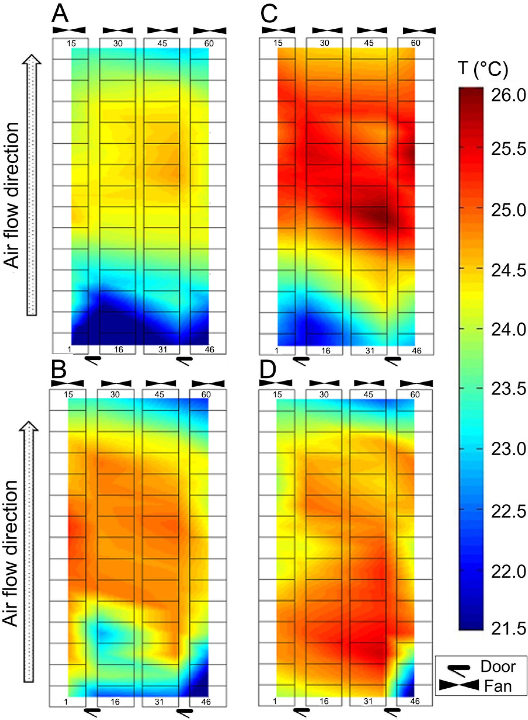
Temperature differences between crates were as high as 9.6 °C and 8.6 °C in Room 1 and 2, respectively, when measured at the same instant. Figure 3A, B, C, and D illustrates the temperature distribution among crates for a representative day of summer and winter. Generally, the crates located in the centre towards the fan end of the farrowing rooms were warmer (p < 0.05) than crates located near the opposite end of the rooms during summer (Figure 3A and C), whereas during winter, temperature levels were higher (p < 0.05) towards the centre of the farrowing rooms and lower near fans and doors (Figure 3B and D). This temperature distribution is typical of tunnel ventilated animal housing, where the intake air exchanges heat with the environment and animals as it flows from one end of the barn to the opposite end, reaching the exhaust fans at higher temperatures.

Figure 3
Farrowing Rooms 1 (A and B) and 2 (C and D). Top view, not to scale. Temperature (T), distribution among crates for a representative day and time during summer (A and C) and winter (B and D). Respective measurement day and times: A) Replicate 26, 13 June 2014, 7h56; B) Replicate 18, 12 Jan 2014, 13h41; C) Replicate 27, 26 June 2014, 8h20; D) Replicate 19, 26 Jan 2014, 15h32. Crate numbers at the bottom start at 1, 16, 31 and 46 from left to right and increase upwards.

Keeping sows and piglets within their thermal comfort zones in conventional farrowing crates is challenging, even in thermally controlled environments, as sows can be heat stressed above 22 °C (Quiniou and Noblet, 1999), whereas piglets feel comfortable within the range of 29.0 °C to 34.0 °C (Johnson and Marchant-Forde, 2009; Lossec et al., 1998; Renaudeau et al., 2003). While heat stressing sows has negative behavioral, physiological and productivity consequences (Quiniou and Noblet, 1999; Renaudeau and Noblet, 2001), piglets commonly experience a 2.0 °C to 4.0 °C drop in body temperature at birth and, if not provided with enough heat, excessive hypothermia may lead to reduced vigour, reduced colostrum and milk intake, and eventually death (Lossec et al., 1998).

Thus, the sows in this study were likely to be heat stressed for most of the summer, as average daily temperatures reached levels above 28.0 °C in both rooms (Figure 2A and B), as they were at or above 22.0 °C for 100 % of the summer in both rooms (Figure 2C and D). On the other hand, a number of the piglets studied may have been cold stressed when not using the heated mat and lamps, as daily temperatures fell to a minimum average of 15.6 °C in Room 1 (Figure 2A) with 100 % of winter being at or below 25.0 °C in both rooms studied (Figure 2C and D). Moreover, Figure 3A, B, C, and D show areas in both rooms where some of the sows would be thermally comfortable, while other sows could have been experiencing heat stress in different areas of the room at the same time.

Relative humidity - seasonal, daily, and room variation

Average relative humidity during winter was approximately 10 % to 16 % lower (p < 0.05) than during summer in both Rooms 1 and 2, respectively. Overall, mean relative humidity in Room 1 (62 ± 11 %) was slightly (3 %) lower (p = 0.03) than the overall year average relative humidity for Room 2 (65 ± 10 %). Although the maximum difference in mean relative humidity between rooms and seasons did not surpass 16 %, relative humidity frequency distribution over the year varied substantially between farrowing rooms. Room 1, for example, spent nearly twice as much time (45 % of summer) as Room 2 at or below 60 % relative humidity (Figure 4A, B, C, and D).

Figure 4
Mean relative humidity (RH) for each experimental day in Room 1 (A) and Room 2 (B); frequency distribution of mean daily RH by season in Room 1 (C) and Room 2 (D). Summer = 1 July to 21 Sept 2013 and 12 to 27 June 2014; Winter = 13 Dec 2013 to 21 Mar 2014; Fall/Spring = 13 to 19 May 2013 (Spring); 21 Sept to 6 Dec 2013 (Fall); and 30 Mar to 30 Apr 2014 (Spring).

Relative humidity - within day and within room variation

Relative humidity differences between crates were as high as 57 % and 49 % in Room 1 and 2, respectively, when measured at the same instant. Figure 5A, B, C, and D illustrates the relative humidity distribution between crates for a representative day of summer and winter. Overall, crates 16 and 46 often had the highest (p < 0.05) relative humidity in Room 1 both in summer and winter, while relative humidity spatial distribution in Room 2 was more variable from crate to crate. The frequent high levels of relative humidity found near the door end of Room 1 and in some instances during summer in Room 2 (Figure 5A, B, and C) were possibly attributable to these crates being next to water hoses in the room, used daily to wet the feed and for boot and equipment washing in the room. Thus, direct water manipulation inside the far-rowing rooms may have contributed to increasing relative humidity levels in the room. It is also possible that manipulation of the drinker by the sow also contributed to the increase in variable relative humidity, along with the animals' respiration, as well as evaporation from the pit and surfaces.

Figure 5
Farrowing Rooms 1 (A and B) and 2 (C and D). Plan view, not to scale. Relative Humidity (RH), distribution among crates for a representative day and time during summer (A and C) and winter (B and D). Respective measurement day and times: A) Replicate 4, 27 July 2013, 9h25; B) Replicate 16, 16 Dec 2013, 10h47; C) Replicate 3, 14 July 2013, 10h58; D) Replicate 19, 25 Jan 2014, 14h47. Crate numbers at the bottom start at 1, 16, 31 and 46 from left to right and increase upwards.

High relative humidity reduces the efficiency of heat loss through evaporation and adds heat to the air, all of which can contribute to pig heat stress when combined with high ambient temperatures. Huynh et al. (2005), for example, demonstrated that high relative humidity levels of 80 % accentuated the reduction in the pig's voluntary feed intake and increase in respiration rate. Sows and piglets of distinct crates in this study were likely to be experiencing different thermal environments, caused by differences in both ambient temperature and relative humidity between crates as presented in this research.

Light intensity - seasonal, daily, and room variation

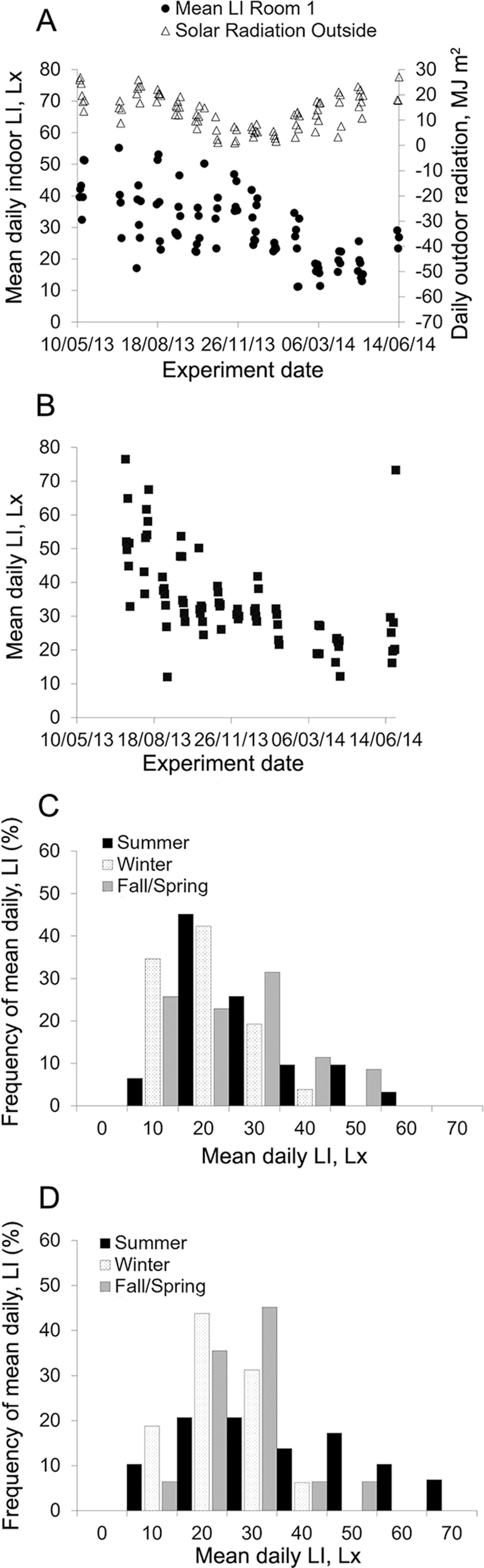
Average light intensity in summer was approximately 9.5 Lx and 13.8 Lx higher (p < 0.05) than in winter in Rooms 1 and 2, respectively. Additionally, average light intensity in Room 1 (29.8 ± 11.2 Lx) was slightly (4.8 Lx) lower (p = 0.01) than the overall annual average light intensity for Room 2 (34.6 ± 13.8 Lx). Although the difference in mean light intensity between rooms was low and light intensity was kept within 20.0Lx and 50.0 Lx for most of the year (Figure 6A and B), light level distribution differed between rooms over summer. While Room 1 had a mean daily light intensity between 10.0 Lx and 30.0 Lx for over half of the summer days (Figure 6C), Room 2 had this light range for 31 % of the summer days, 30.0 Lx to 50.0 Lx for 35 % of the summer days with the remaining 34 % of the summer days from 50 Lx to 70.0 Lx (Figure 6D).

Figure 6
Mean light intensity (LI) for each experimental day in Room 1 and daily solar radiation outdoors (A); mean LI in Room 2 (B); frequency distribution of mean daily LI by season in Room 1 (C) and Room 2 (D). Summer = 1 July to 21 Sept 2013 and 12 to 27 June 2014; Winter = 13 Dec 2013 to 21 Mar 2014; Fall/Spring = 13 to 19 May 2013 (Spring); 21 Sept to 6 Dec 2013 (Fall); and 30 Mar to 30 Apr 2014 (Spring).

The overall decrease in daily light intensity as months turned colder could be a consequence of a reduced influence of external light sources during this period and thus reduced radiation after summer (Figure 6A). Additionally, fluorescent light bulbs decrease their luminosity over time, which could be one possible reason for the light intensity means to have remained at lower levels in the summer of 2014, compared to the summer of 2013.

Light intensity - within day and within room variation

Light intensity differences between crates were as high as 3,847.3 Lx and 2,255.0 Lx in Room 1 and 2, respectively, when measured at the same instant. Figure 7A, B, C, and D illustrates the light intensity distribution between crates for a representative day of summer and winter. The crates that most frequently captured the highest light intensity in the room during summer were either near the fan end and the door end. During winter, the crate which captured the highest light intensity in Room 1 was crate 29, which is also near the fan end, while in Room 2, crates which captured the highest light intensity the most frequently were more spread apart (crates 33, 41, and 44).

Figure 7
Farrowing Rooms 1 (A and B) and 2 (C and D). Plan view, not to scale. Light intensity (LI), distribution among crates for a representative day and time during summer (A and C) and winter (B and D). Respective measurement day and times: A) Replicate 2, 3 July 2013, 13h45, B) Replicate 16, 14 Dec 2013, 7h07, C) Replicate 5, 7 Aug 2013, 6h50, D) Replicate 17, 27 Dec 2013, 6h20. Crate numbers at the bottom start at 1, 16, 31 and 46 from left to right and increase upwards.

The position of crates capturing the highest levels of light intensity in Room 1 near the door and fan ends suggests that external light, coming through the doors and fans, affected the light intensity environment of the crates near those ends in Room 1. Conversely, Room 2 seemed to be less affected by external light, possibly due to its position relative to the other rooms, as Room 2 shared only one wall with the exterior, while Room 1 had two external walls.

The light schedule has been reported to affect sow behavior and reproduction (McGlone et al., 1988; Prunier et al., 1994). Though little is known about the effects of light quality and intensity on the behavior of pigs, it is known that pigs which were trained to recognize symbols failed to do so below 20.0 Lx of light intensity (Zonderland et al., 2008). Thus, sows in this study experienced a distinct proportion of time during their 48 h post-partum during which they could clearly see and periods of time during which they were probably not able to completely visually perceive their surroundings. Moreover, when compared at the same instant, sows of distinct crates had entirely different visual perceptions due to different light levels in their crates.

Sound intensity - seasonal, daily, and room variation

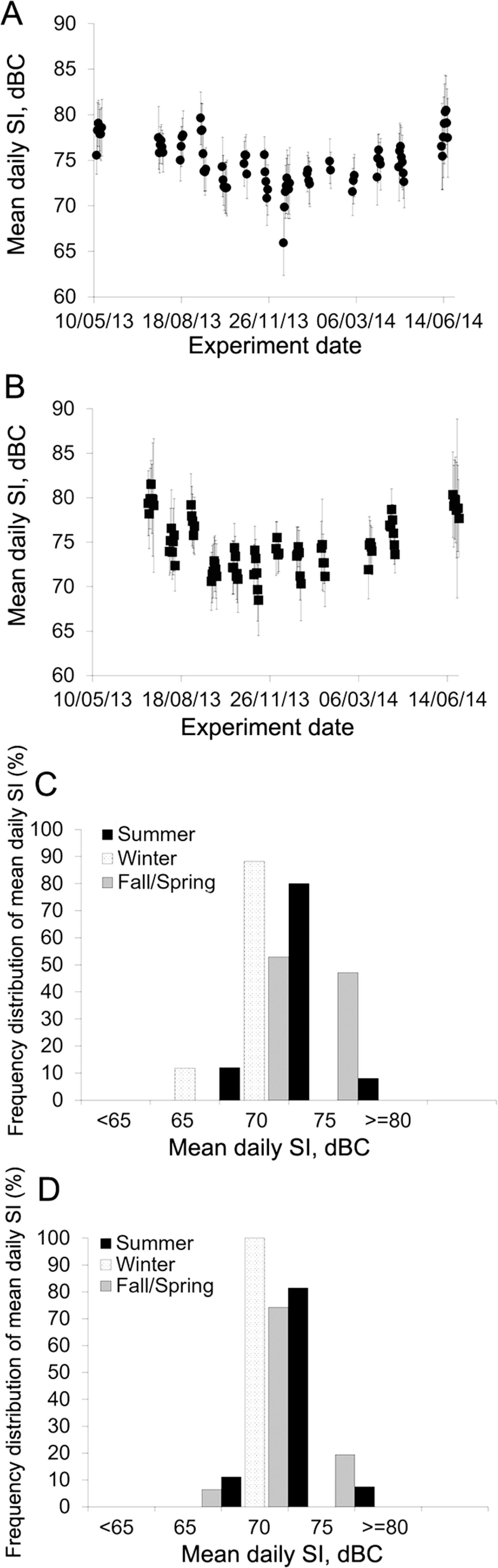
Sound intensity was approximately 5.0 dBC and 4.5 dBC lower (p < 0.05) during winter as compared to summer in Room 1 and 2, respectively. Although there was no difference in mean sound intensity between rooms (p = 0.90), there was a substantial variation in sound levels throughout the year, as illustrated in Figure 8A, B, C, and D. Sound intensity during winter was mostly between 65.0 dBC and 75.0 dBC in both rooms, while during summer, they were between 75.0 dBC and 80.0 dBC for at least 80 % of the summer days in both rooms (Figure 8C and D).

Figure 8
Mean sound intensity (SI) for each experimental day in Room 1 (A) and Room 2 (B); frequency distribution of mean daily SI by season in Room 1 (C) and Room 2 (D). Summer = 1 July to 21 Sept 2013 and 12 to 27 June 2014; Winter = 13 Dec 2013 to 21 Mar 2014; Fall/Spring = 13 to 19 May 2013 (Spring); 21 Sept to 6 Dec 2013 (Fall); and 30 Mar to 30 Apr 2014 (Spring).

Mean daily sound intensity levels found in this study were above those found by Sampaio et al. (2007) in their study on nursery and finishing facilities, but were in agreement with Talling et al. (1998) for mechanically ventilated pig barns. The difference in levels found in the current study and Sampaio's study (2007) may be attributable to differences in animal age, stocking density, physical environment, as well as environmental controls. Sampaio et al. (2007) conducted their experiments in Brazil, where swine facilities tend to be more open, utilizing less mechanical ventilation as compared to the farm studied in this research. Also, naturally ventilated buildings were demonstrated to be approximately 10 dB quieter than mechanically ventilated buildings (Talling et al., 1998).

Sound intensity - within day and room variation

Sound intensity differences between crates were as high as 38.7 dBC and 24.3 dBC in Room 1 and 2 respectively when measured at the same instant. Figure 9A, B, C, and D illustrates the sound intensity distribution among crates for a representative day of summer and winter. Generally, the crates located in the centre towards the fan end of the farrowing rooms had higher sound levels (p < 0.05) than those located near the door end of the rooms during summer, whereas during winter the sound intensity gradient between the fans and door end was not as pronounced. The variation in sound intensity in this research was associated with the variation in air velocity, as evidenced by the strong (80 %, p< 0.01) positive correlation found between mean air velocity and sound intensity in both rooms studied. Therefore, a great portion of the sound intensity recorded in the farrowing rooms was generated by the fans when they were in operation, leading to an increase in sound intensity in warmer months near the fan end of the room.

Figure 9
Farrowing Rooms 1 (A and B) and 2 (C and D). Plan view, not to scale. Sound intensity (SI), distribution among crates for a representative day and time during summer (A and C) and winter (B and D). Respective measurement day and times: A) Replicate 8, 9 Sept 2013, 19h02, B) Replicate 21, 3 Mar 2014, 18h59, C) Replicate 3, 15 July 2013, 19h01, D) Replicate 19, 24 Jan 2014, 19h02. Crate numbers at the bottom start at 1, 16, 31 and 46 from left to right and increase upwards.

The implications of environmental sound intensity in swine farrowing rooms is not entirely understood. Hutson et al. (1993) demonstrated that the intensity of the piglet squeal is relevant for sow responsiveness. The authors reported that louder squealing (over 92.0 dB) was associated with the sow lying down slowly while kneeling, which could decrease piglet crushing (Andersen et al., 2005; Burri et al., 2009). Additionally, Talling et al. (1996) demonstrated that exposure to ambient sounds of 80.0 dB to 97.0 dB can trigger the activation of the defence mechanisms in pigs, while music can be used as a tool to improve the welfare of weaned piglets (Jonge et al., 2008). Therefore, it may be interesting from a production and welfare perspective to further investigate the effects of environmental noise and loudness on piglet survivability, behavior, and maternal behavior of sows, such as responsiveness.

Air velocity - seasonal, daily, and room variation

Air velocity was approximately 0.10 m s^–1 and 0.14 m s^–1 lower (p < 0.05) during winter compared to summer in Rooms 1 and 2, respectively. Mean daily air velocity levels reached a minimum and a maximum of 0.05 m s^–1 and 0.28 m s^–1 in Room 1, as well as a minimum and maximum level of 0.08 m s^–1 and 0.40 m s^–1 in Room 2. The frequency distribution of air velocity levels varied between summer and winter in both rooms (Figure 10A, B, C, and D). Crate air velocity during winter was mostly (at least 80 % of time) below 0.10 m s^–1 in both rooms, while during summer air velocity levels were mostly (79 %) within a range of 0.10 m s^–1 and 0.20 m s^–1 in Room 1, and above 0.20 m s^–1 for 61 % of the summer in Room 2 (Figure 10C and D).

Figure 10
Mean air velocity (AV) for each experimental day in Room 1 (A) and Room 2 (B); frequency distribution of mean daily AV by season in Room 1 (C) and Room 2 (D). Summer = 1 July to 21 Sept 2013 and 12 to 27 June 2014; Winter = 13 Dec 2013 to 21 Mar 2014; Fall/Spring = 13 to 19 May 2013 (Spring); 21 Sept to 6 Dec 2013 (Fall); and 30 Mar to 30 Apr 2014 (Spring).

Little is known about the isolated effects of air velocity on pig welfare. Higher air velocity levels (0.30 m s^–1) have been previously reported to be preferred by weaned piglets (Geers et al., 1986) and 0.15 m s^–1 to 0.40 m s^–1 air velocities were shown to improve pen hygiene of 60 kg to 90 kg pigs (Sallvik and Walberg, 1984). The air velocity estimates of the present study suggest that pigs did not experience crate air velocity of 0.30 m s^–1 or above this level in Room 1 (Figure 10C), while pigs in Room 2 experienced this range of air velocity for 22 % of the summer (Figure 10D). Additionally, it is possible that the air velocity experienced by the sows in this experiment was even lower than the values reported in this study, due to potential obstructions in the air flow, caused by the pen partitions and metal structures around the sows. Despite the few reports in the literature about the direct effects of air velocity on pig welfare, it is known that air velocity directly contributes to the pigs' thermoregulation. Thus, it may be useful to take air velocity into consideration within the pig's microenvironment, especially in conventional swine farrowing rooms, where crated animals cannot choose between higher versus lower air velocity sites.

Air velocity - within day and room variation

Figure 11A, B, C, and D displays the air velocity across Room 1 for Fan Setting 1 and 5. Crates 1 to 15 and 16 to 30 in Room 1 had relatively lower (p < 0.01) air velocities than the remaining crates at fan setting 3 and above. Air velocities in Room 2 were higher (p < 0.01) at crates near the fan end of the room as compared to the crates near the door end at fan setting 3 and above. Maximum crate air velocity difference when measured at the same instant was 0.15 m s^–1 and 0.13 m s^–1 in Rooms 1 and 2, respectively. The higher air velocities found near the fan end in Room 2 were expected, as the volume of air being moved by the fans converged to pass through the fans, thus increasing air speed near the fans. However, the lower air velocities on crate rows one to 15 and 16 to 30 were not expected and may have been caused by differences in the air inlets' settings or fan performance.

Figure 11
Farrowing Room 1 (A and B) and Room 2 (C and D), plan view, not to scale. Air velocity (AV), distribution among crates at Fan Stage 1 with two pit fans running (A and C) and Fan Stage 5 with all fans running (B and D). Crate numbers at the bottom start at 1, 16, 31 and 46 from left to right and increase upwards.

Conclusions

The present research described the variation in temperature, relative humidity, light intensity, sound intensity, and air velocity between two (60 crate) commercial farrowing rooms over 1 year of operation. When looking only at the means reported, all the variables measured seemed to be within common farm levels for most of the days studied. However, spatial distributions revealed that differences between distinct crates were as high as 9.6 °C, 57 %, 3,847.3 Lx, 0.87 m s^–1, and 38.7 dBC when measured at the same instant inside a room. Moreover, frequency distributions demonstrated that the proportion of time spent by the pigs within distinct levels of all measured variables substantially differed between the two rooms studied, despite their similarity. The data suggested that some of the sows in this experiment could have been thermally comfortable or better able to visually perceive their environment, while others could have experienced heat stress or lack of visibility at the same time in different areas of the rooms. Similarly, some of the sows experienced higher levels of relative humidity, air velocity, and sound, while others were in a quieter, less drafty, and less humid environment in the room at the same time. Additionally, environmental measurements reached levels which were unexpected and potentially harmful to the welfare of both sows and piglets, such as the low average temperature of 15.6 °C reported for Room 1 in winter. It is suggested, therefore, that future research focus on the development of environmental controls which take into account the microenvironments existing in commercial farrowing rooms, considering that more localized areas for the control of temperature, humidity, sound, light, and air velocity may contribute to a reduction in production variability as a possible consequence of environmental variability. Moreover, microenvironments should also be considered during research studies, where environmental variation could potentially explain part of the variation in the response variables being measured on the animals.

Acknowledgements

The authors would like to thank the USDA-ARS Livestock Behavior Research Unit for funding and supporting the present research, as well as the Purdue Animal Sciences Department and the MP3 Farms for their support and collaboration.

References

• Andersen, I.L.; Berg, S.; Bøe, K.E. 2005. Crushing of piglets by the mother sow (Sus Scrofa) purely accidental or a poor mother? Applied Animal Behaviour Science 93: 229-243.
• Andersen, I.L.; Tajet, G.M.; Haukvik, I.A.; Kongsrud, S.; Bøe, K.E. 2007. Relationship between postnatal piglet mortality, environmental factors and management around farrowing in herds with loose-housed, lactating sows. Acta Agriculturae Scandinavica, Section A: Animal Science 57: 38-45.
• Baxter, E.M.; Lawrence, A.B.; Edwards, S.A. 2012. Alternative farrowing accommodation: welfare and economic aspects of existing farrowing and lactation systems for pigs. Animal 6: 96-117.
• Burri, M.; Wechsler, B.; Gygax, L.; Weber, R. 2009. Influence of straw length, sow behaviour and room temperature on the incidence of dangerous situations for piglets in a loose farrowing system. Applied Animal Behaviour Science 117: 181-189.
• Carvalho, T.M.R.; Moura, D.J.; Souza, Z.M.; Souza, G.S.; Bueno, L.G.F.; Lima, K.A.O. 2012. Use of geostatistics on broiler production for evaluation of different minimum ventilation systems during brooding phase. Revista Brasileira de Zootecnia 41: 194-202.
• Faria, F.F.; Moura, D.J.; Souza, Z.M.; Matarazzo, S.V. 2008. Climatic spatial variability of a dairy freestall bar. Ciência Rural 38: 2498-2505 (in Portuguese, with abstract in English).
• Geers, R.; Goedseels, V.; Parduyns, G.; Vercruysse, G. 1986. The group postural behaviour of growing pigs in relation to air velocity, air and floor temperature. Applied Animal Behaviour Science 16: 353-362.
• Gu, Z.; Gao, Y.; Lin, B.; Zhong, Z.; Liu, Z.; Wang, C.; Li, B. 2011. Impacts of a freedom farrowing pen design on sow behaviours and performance. Preventive Veterinary Medicine 102: 296-303.
• Hutson, G.D.; Price, E.O.; Dickenson, L.G. 1993. The effect of playback volume and duration on the response of sows to piglet distress calls. Applied Animal Behaviour Science 37: 31-37.
• Huynh, T.T.T.; Aarnink, A.J.A.; Gerrits, W.J.J.; Heetkamp, M.J.H.; Canh, T.T.; Spoolder, H.A.M.; Kemp, B.; Verstegen, M.W.A. 2005. Thermal behaviour of growing pigs in response to high temperature and humidity. Applied Animal Behaviour Science 91: 1-16.
• Johnson, A.K.; Marchant-Forde, J.N. 2009. Welfare of pigs in the farrowing environment. p. 141-188. In: Marchant-Forde, J.N., ed. The welfare of pigs. Springer, Amsterdam, Netherlands.
• Jonge, F.H.; Boleij, H.; Baars, A.M.; Dudink, S.; Spruijt, B.M. 2008. Music during play-time: using context conditioning as a tool to improve welfare in piglets. Applied Animal Behaviour Science 115: 138-148.
• Lossec, G.; Herpin, P.; Le Dividich, J. 1998. Thermoregulatory responses of the newborn pig during experimentally induced hypothermia and rewarming. Experimental Physiology 83: 667-678.
• Marchant-Forde, J.N.; Broom, D.M.; Corning, S. 2001. The influence of sow behaviour on piglet mortality due to crushing in an open farrowing system. Animal Science 72: 19-28.
• McGlone, J.J.; Morrow-Tesch, J. 1990. Productivity and behavior of sows in level vs. sloped farrowing pens and crates. Journal of Animal Science 68:82-87.
• McGlone, J.J.; Stansbury, W.F.; Tribble, L.F.; Morrow, J.L. 1988. Photoperiod and heat stress influence on lactating sow performance and photoperiod effects on nursery pig performance. Journal of Animal Science 66: 1915-1919.
• Prunier, A.; Dourmad, J.Y.; Etienne, M. 1994. Effect of light regimen under various ambient temperatures on sow and litter performance. Journal of Animal Science 72: 1461-1466.
• Quiniou, N.; Noblet, J. 1999. Influence of high ambient temperatures on performance of multiparous lactating sows. Journal of Animal Science 77: 2124-2134.
• Renaudeau, D.; Noblet, J. 2001. Effects of exposure to high ambient temperature and dietary protein level on sow milk production and performance of piglets. Journal of Animal Science 79: 1540-1548.
• Renaudeau, D.; Noblet, J.; Dourmad, J.Y. 2003. Effect of ambient temperature on mammary gland metabolism in lactating sows. Journal of Animal Science 81: 217-231.
• Sallvik, K.; Walberg, K. 1984. The effects of air velocity and temperature on the behaviour and growth of pigs. Journal of Agricultural Engineering Research 30: 305-312.
• Sampaio, C.A.P.; Nääs, I.A.; Salgado, D.D.; Queirós, M.P.G. 2007. Evaluation of the noise level in swine housing. Revista Brasileira de Engenharia Agrícola e Ambiental 11: 436-440 (in Portuguese, with abstract in English).
• Stalder, K.J. 2013. Pork Industry Productivity Analysis. Iowa State University, Des Moines, IA, USA.
• Talling, J.C.; Lines, J.A.; Wathes, C.M.; Waran, N.K. 1998. The acoustic environment of the domestic pig. Journal of Agricultural Engineering Research 71: 1-12.
• Talling, J.C.; Waran, N.K.; Wathes, C.M.; Lines, J.A. 1996. Behavioural and physiological responses of pigs to sound. Applied Animal Behaviour Science 48: 187-202.
• Zonderland, J.J.; Cornelissen, L.; Wolthuis-Fillerup, M.; Spoolder, H.A.M. 2008. Visual acuity of pigs at different light intensities. Applied Animal Behaviour Science 111: 28-37.

Edited by

Edited by: Paulo Cesar Sentelhas

Publication Dates

• Publication in this collection
  Jan-Feb 2018

History

• Received
  31 July 2016
• Accepted
  15 Nov 2016