Data processing within rows for sugarcane yield mapping

ABSTRACT:

The mapping of sugarcane yield is still not as widely available as it is for grain crops. Sugarcane harvesters cut and process the cane in a single or maximum of two rows, facilitating the monitoring of cane yield and its behavior on a small scale. This study tested a method for sugarcane yield data cleaning, investigating if the data recording frequency influences the characterization of yield variations in mapping high-resolution spatial data within a single row. Four data sets from yield monitors of single row harvesting were used. A cleaning process with global and anisotropic filtering in a single sugarcane row was applied. The local outlier cleaner compares the yield value of a point with its nearest neighbors within the same row. Even after the elimination of outliers, there is great variation in yield between the rows, and this variation is much smaller in a single row. A frequency of 2 Hz was required for identifying and characterizing small yield variations within the sugarcane rows whilst other frequencies tried (0.2 and 0.1 Hz) resulted in loss of information on yield variability within the row. The difference between the root mean square error (RMSE) of ordinary kriging (OK) and inverse distance weighting (IDW) techniques is large enough to suggest the use of an individual yield line. Individual yield lines saved information in the data generated by the yield monitor unlike IDW and OK interpolation methods which omitted information over short distances within the rows and compromised the quality of high-resolution maps.

Keywords:
yield monitor; sugarcane variability; line maps

Introduction

Sugarcane (Saccharum spp.) has a high production cost. Information on yield and production costs is essential to the management of agricultural fields (Griffin et al., 2018). The mapping of sugarcane yields converts estimates into quantitative values that can be more easily used by decision-makers (Fernandes et al., 2017). These maps allow farmers to determine yield variations and investigate the causes of these variations (Price et al., 2017). According to Amaral et al. (2018), sugarcane has high biomass variability in adjacent rows. Therefore, a yield monitor installed on a sugarcane harvester, which cuts and processes the cane harvested along a single or double row, might offer a means of producing high-resolution yield data and, consequently, high-resolution maps.

Yield spatial information on individual lines can be an option for mapping yield variability within sugarcane rows, thus offering the potential, for example, to create nutrient export maps for site-specific variable rate application, row by row. However, the data produced by the yield monitors present systematic errors in the data set, and post-processing is necessary to eliminate these errors before making the maps (Leroux et al., 2018; Driemeier et al., 2016; Lyle et al., 2014). Different methods that apply sequences of filters, which classify, identify, and remove spatial outliers of grains yield data, have been developed in the past (Vega et al., 2019; Leroux et al., 2018; Spekken et al., 2013; Sudduth and Drummond, 2007; Menegatti and Molin, 2004; Blackmore and Moore, 1999). These methods use statistical parameters to classify a given point in the data set by taking into account points on neighboring rows. Thus, yield data processing already used for other crops can exclude data with useful information on spatial variability within the sugarcane row. Given this possibility, it is necessary to understand the real quality of the data and how they express yield variability within the field and, in particular, within every single row. Furthermore, it is worth investigating if data density provided by yield monitors influences the characterization of yield variations within the same row. Therefore, this study hypothesized that greater resolution of data variability within sugarcane rows can reveal information that might substantially support farmers in their decisions in the field through the use of high-resolution yield maps. Thus, the current study aimed to (i) test a method for sugarcane yield data cleaning; (ii) investigate if data recording frequency influences characterization of yield variations within the same row; and (iii) create high-resolution yield line maps.

Materials and Methods

Four yield data sets from sugarcane fields in the central-western region of the state of São Paulo, Brazil (21° 21′ S, 48°40′ W; 523 m altitude) were used. Scale yield monitors installed on the harvester elevator generated the data, measuring the amount of sugarcane that passes through the conveyor before being dumped into the infield wagon (Mailander et al., 2010; Jensen et al., 2013). Due to the use of two monitors, each from different manufacturers, data sets were recorded with different frequencies (Table 1). The two yield monitors were set up to record data at the highest frequency allowed by the equipment. The harvesting was carried out in fields with 1.5 m spacing between rows.

Table 1
Data set characterization.

Data	Area	Frequency	N° points	Density	Distance	Average yield
	ha	Hz		points ha−1	m	Mg ha−1
Field 1	15.7	0.2	26877	1711.9	2.8	137.4
Field 2	9.8	0.2	13255	1352.6	3.1	105.8
Field 3	3.6	1.0	17237	4788.1	1.2	243.6
Field 4	8.7	1.0	62426	7175.3	1.0	250.6

Each yield monitor data set was subjected to a sequential data screening in order to detect and remove points with erroneous values. This process was implemented in three stages.

Step 1- Global filter

Data were screened by filtering zero yield values and global outliers (Vega et al., 2019; Sudduth and Drummond, 2007). The global filtering method for identifying outliers is the Interquartile Range (IQR) (Tukey, 1977). The IQR is the range between the first and the third quartiles. Tukey (1977) therefore considered any data point that fell outside 1.5 times the IQR below the first quartile or 1.5 times the IQR above the third quartile to be outliers (Figure 1).

Figure 1
Steps for cleaning data set and procedure for yield line maps.

Step 2 – Identify rows

Based on the assumption that sugarcane harvesters run through sites in an alternating round trip (Jin and Tang, 2010), row separation was obtained by the method described by Lyle et al. (2014). The direction of the harvester was determined, and every change in direction was considered the beginning of a new row.

Step 3 – Local anisotropic filter

In addition to the data remaining after global filtering, two parameters had to be provided as inputs for the model. Local filtering allows the user to identify and eliminate points that cause yield variation within a set of neighboring points and preserve points with consistent yield values (Vega et al., 2019; Leroux et al., 2018; Spekken et al., 2013).

The local filtering method proposes detecting all points located in a radius range (R_i) around a point (P_i) within a single sugarcane row (red polygon Figure 1). For the four data sets, points located at a R_i ≤ 21 m were used. This was the smallest range of spatial data dependence found among the four data sets. The model assumes that the defined radius range does not exceed the spatial data dependency. However, due to the speed of the harvester and the frequency of the data logger, the distance between collected points will vary, and therefore, users can set this radius range according to the data set they want to filter. In the sequence, the median of these points is calculated. If the yield value in P_i is above the upper limit (Eq. 1) or below the lower limit (Eq. 2), it is considered an outlier and is filtered out.

(1) $$UL=Med+Med\mathrm{x}var$$

(2) $$LL=Med–Med\mathrm{x}var$$

where: UL is the upper limit, LL the lower limit, Med, the median of all points located in R_i, and var, the maximum variation accepted for the median. By default, the maximum variation acceptable for the four data sets was 20 %. The process is repeated for each point in the data set. All related functions of identifying and removing discrepant data were programmed using the Python programming language. The python script was run in a multi-purpose open source geographic information system (QGIS Geographic Information System, v. 2.18, QGIS, 2018).

A geostatistical analysis was carried out to characterize the spatial variability of the sugarcane yield in order to verify differences in spatial dependence across and within the rows. An anisotropic analysis was performed using both all values of the data set and those for each row individually taking into account only data within a single row. Semivariograms were individually modeled, testing the spherical, exponential and gaussian models, to ultimately choose the one with the lower root mean square error (RMSE, Eq. 3) of cross-validation results (Isaaks and Srivastava, 1989). The spatial dependence was evaluated based on the nugget effect percentage on the sill variance, and it was classified as strong (< 25 %), moderate (between 25 and 75 %), or weak (> 75 %) (Cambardella et al., 1994). The semivariograms were modeled using the R 3.3.3 program (R Core Team, 2017) and the geoR package version 1.7-5.1 (Ribeiro Júnior and Diggle, 2001).

(3) $$RMSE=\sqrt{\frac{1}{n}{{\displaystyle {\sum }_{i=1}^n\left\{Z(xi)-\widehat{Z}(xi)\right\}}}^2}$$

where $\widehat{Z}(xi)$ is the predicted value; Z(xi), the observed (known) value; and n, the number of values in the data set (Robinson and Metternicht, 2006).

A simulation with the recording frequency was conducted to determine if it influences the identification of small yield variation within the row using the filtered data of field 3, with common frequencies for yield monitors, as follows: each point (1 Hz as reference), dropping out one of every two points (0.5 Hz), dropping out four of every five points (0.2 Hz) and adding one point in the middle of two points (2 Hz). The influence of frequency on the data collected was quantified by evaluating the changes of semivariogram parameters between the reference (1 Hz) and simulated frequencies. The semivariograms were fitted, and the prediction quality after applying the simulated frequencies assessed using cross-validation (James et al., 2014).

In order to generate information similar to that in the original data, individual yield lines were created with georeferenced yield values for each crop row using the ‘Points2One’ QGIS tool to extract the line (harvester path) from the layer of points generated by the yield monitor. The harvester runs through the field in parallel rows. Thus, the ‘Editspline’ tool from AutoCAD software 2017 (California, United States) was used to smooth out the lines generated, and the ‘Offset’ tool was used to make them parallel in order to remove the minor deviations in the harvester path, due to Global Navigation Satellite System (GNSS) errors. The lines generated were broken at nodes every 0.5 m, which represents a maximum distance without plants but greater than that may be considered as a gap (Stolf, 1986).

To estimate yield values in the lines, the ‘Voronoi Polygons’ tool from QGIS software was used. This algorithm divides the area into smaller polygons, each corresponding to the coverage area of each point in the processed data set. Finally, the values of the polygons in the line layer were joined using the ‘Intersection’ tool from QGIS. This tool makes layer overlays (line and Voronoi polygon) for the output file (line) to record values where both layers intersect. To verify the impact of the proposed line map protocol, a comparison of line maps with surface maps generated by OK and the IDW interpolation methods was made. To compare different interpolation techniques, the difference between the known data and the predicted data using the RMSE (Eq. 3) was examined. The RMSE is a measure of the average magnitude of the estimated errors, always has a positive value and, being closer to zero, suggests a higher quality of the measured or estimated values.

Results and Discussion

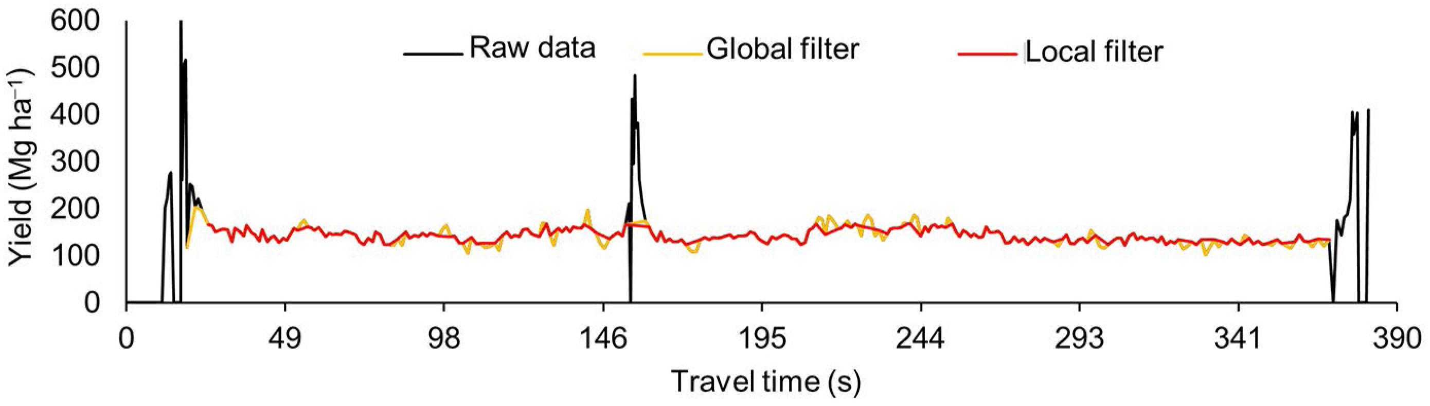
Sugarcane harvesters carried out the cutting, fractioning, partial cleaning, and loaded the stalks directly into the infield wagon, whose driving was synchronized with the harvester. Maneuvering time of the harvester was shorter than that of the wagon and in certain situations, the harvesting started before synchronization with the wagon. Thus, the conveyor belt remains off (time off - TO) for a period, and there is cane stalk accumulation in the elevator basket, causing the yield monitor to record zero values (Figure 2A). High yield data is recorded by activating the conveyor belt.

Figure 2
Error in yield data at the beginning of a new row (A) and during wagon replacement in the middle of the field (B). Black arrows represent the direction of the harvester path. YV = yield variation; TO = elevator time off; ST = sugarcane flow stabilization time.

In the data sets studied, the average flow stabilization time (ST) in the conveyor belt was 7.0 s and ST varied according to TO; a greater amount of cane harvested with the conveyor belt off resulted in greater ST. This error also occurred with wagon replacement in the middle of the field (Figure 2B). Positioning errors and data logging errors during machine maneuvers can be observed at the end of the path in Figure 2A. The yield monitor recorded a large quantity of data with both position and zero yield values during maneuvers (red points in Figure 2A).

The harvesting width was fixed; however, high variance in yield values in small distances within the row could be observed indicating the presence of discrepant data. The median values deviate from values of the mean, and the minimum and maximum values reinforce high data variability. These present high values of the coefficient of variation (Table 2), which may be considered as the first indicator of data set heterogeneity.

Table 2
Yield descriptive statistics of original and processed data sets.

Field	Type	n	n excluded	Min	Mean	Median	Max	SD	CV	sk	ku
				------------------------------------------- Mg ha−1 -------------------------------------------					%
1	Or	26877		–42.8	137.4	130.8	1172.0	67.5	49.1	1.6	9.8
	Proc	21096	5781 (22 %)	20.4	131.8	128.5	297.2	45.3	34.4	0.4	–0.1
2	Or	13255		–11.8	105.8	96.0	1366.8	58.0	54.8	4.0	39.2
	Proc	11142	2113 (16 %)	29.5	94.7	91.6	217.3	30.2	31.9	0.5	–0.2
3	Or	17237		0.0	243.6	201.5	35587.0	1251.3	513.7	21.8	524.4
	Proc	11968	5269 (31 %)	103.8	216.1	211.8	349.3	31.4	14.5	0.7	1.3
4	Or	62425		0.0	250.6	184.9	28092.6	1135.3	453.0	15.8	281.3
	Proc	37675	24750 (40 %)	100.0	208.4	207.1	380.0	45.8	22.0	0.3	0.1

• Or = original data; Proc = processed data; SD = standard deviation; CV = variation coefficient; sk = skewness; ku = kurtosis.

The proposed methodology identified 25 and 15 % of the data as outliers for fields 1 and 2, and 31 and 40 % for fields 3 and 4, respectively, thus excluding them (Table 2). The quantity of data removed was larger than what is normal on cleaning done in grain yield data (Vega et al., 2019). The quantity of data with errors of TO and ST is proportional to the number of harvester paths in the harvested field. Generally, the sugarcane harvester has a smaller harvest width than grain harvesters; consequently, there is more path. This may be the reason for the greater exclusion of outliers in the cleaning process in sugarcane yield data. The larger number of points eliminated in fields 3 and 4 compared to fields 1 and 2 is related to a higher frequency of points collected during harvesting. The global filter removed points with yield values both below 15.3, 18.2, 2.3, and 4.9 Mg ha⁻¹ and above 300.4, 250.1, 571.5, and 578.0 Mg ha⁻¹ for fields 1, 2, 3, and 4, respectively. The removal of site-specific points and global outliers substantially altered the summary statistics of the yield data sets, decreasing values of standard deviation and yield mean by almost 5 % in fields 1-2 and 12 and 20 % in fields 3-4. This is because of the high values of the points with ST influence far in excess of the zero values of the TO unlike grain yield data filtering where most errors in yield values are below average or close to zero (Vega et al., 2019; Leroux et al., 2018; Spekken et al., 2013; Sudduth and Drummond, 2007; Menegatti and Molin, 2004). The skewness and kurtosis coefficient values (Table 2) suggest that yield distribution of the original data was not normal, indicating that average yield values of the original data were influenced by extreme values. The filtering methodology induced the data to have a normal distribution, due to the removal of data with very low and very high yield values (Figure 3).

Figure 3
Yield variation in the raw data and after the cleaning process.

The elimination of a large number of points may affect information quality. However, the density of points is significantly high, even after the removal of local outlier points, and this was done in order for the variations in lower and higher yield over short distances within the row to be identified. This can be better observed by semivariogram parameters, before and after data set filtering (Table 3). Outliers completely compromised the spatial structure of yield in the sites studied. Fields 1 and 2 presented high values for the nugget effect in the original data, while fields 3 and 4 did not present any spatial dependence. High nugget values were expected, due to, firstly, the large density of points collected by the yield monitor within the row and, secondly, to the high yield variability across the adjacent lines (Amaral et al., 2018). After the data cleaning, the exponential model showed the best fit for fields 2, 3 and 4. Studies with grain clean process showed the same semivariogram adjustments as per the clean data (Vega et al., 2019; Leroux et al., 2018). On the other hand, the Gaussian model presented the best fit for field 1. This result was similar to that of Menegatti and Molin (2004) in which the cleaning process improved the cross-validation of the adjusted Gaussian model, contributing to the characterization of spatial dependence and reducing unexplained variability.

Table 3
Geostatistical analyses of original and processed yield data sets.

Field	Type	Model	C0a	C1b	Range	Cross-Validationc			Spatial dependence
					m	a	b	RMSE
1	Original	Exponential	3390.5	4112.5	26.6	1.5	–64.2	57.5	0.78	Weak
	Processed	Gaussian	1392.4	1805.0	21.7	1.6	–77.6	25.1	0.87	Weak
2	Original	Exponential	2462.7	2789.7	26.23	0.7	26.6	49.1	0.88	Weak
	Processed	Exponential	1722.0	1879.2	43.9	1.2	10.4	32.5	0.92	Weak
3	Original	- d	-	-	-	-	-	-	-	-
	Processed	Exponential	685.3	842.0	23.8	1.0	–0.2	50.7	0.81	Weak
4	Original	- d	-	-	-	-	-	-	-	-
	Processed	Exponential	1151.8	2469.3	48.8	1.0	–0.3	21.1	0.47	Moderate

• ^a
  Nugget effect;
• ^b
  sill;
• ^c
  Leave-one-out cross-validation performed by kriging: a = slope; b = intercept; RMSE = Yield root mean square error;
• ^d
  pure nugget effect - did not fit any models.

The primary aim of filtering the yield errors is to improve the quality of the interpolation and for kriging; any improvement in the data quality is indicated by a reduction in the nugget variance (Robinson and Metternicht, 2005). However, even after the cleaning process, the semivariograms showed very high nugget parameters, demonstrating that there is still great variation in yield over small distances. Other studies comparing the methods for cleaning grain yield data show a decrease in the nugget values after data cleaning (Vega et al., 2019; Leroux et al., 2018; Menegatti and Molin, 2004; Sudduth and Drummond, 2007). Sugarcane yield is highly variable over short distances and is especially influenced by gaps. According to Amaral et al. (2018), skips are related to ratoon damages, diseases, pests, and climate conditions.

Yield in the sugarcane fields presents weak spatial dependence, even after removing the local outliers (Table 3), while field 4 data presented moderate spatial dependence (Cambardella et al., 1994). A study by Amaral et al. (2018) using canopy sensors in every single sugarcane row showed moderate spatial dependence of crop-vigor spatial variability. Higher nugget/sill ratio was related to smaller spatial dependence, which means greater spatial randomness. Weak spatial dependence occurs because of yield randomness between neighboring rows. As this data is densely collected, a low nugget effect would be expected (Amaral et al., 2018) and with less data randomness, stronger spatial dependence would also be expected (Vieira et al., 1983). The semivariograms modeling for each sugarcane row showed that there is less yield variation within rows. It means variation in yield values within the same row was much lower than the yield variation across the rows. This can be best observed in Figure 4, where the nugget effect values of the semivariograms fitted for each row were much lower than the nugget effect value of the global semivariogram (dashed line). This reduction in yield variation within-row can be attributed to the elimination of local outliers by the local cleaning process, smoothing out the yield variation within-row.

Figure 4
Yield geostatistical analyses of each row for each field. *C₀ global - nugget effect value of the global semivariogram (Table 3) fitted using all data from the data set.

The density of points recorded by the yield monitor interferes with the yield variability characterization within rows (Figure 5). The decrease in frequency to 0.2 Hz smoothed yield variation within the row, rendering it incapable of identifying small-scale variability. The frequency decrease to 0.1 Hz (one point every 10 s) led to values that were very different from the other scenarios and lost details, which is not desirable. Investigations for local interventions within the sugarcane row demands knowing yield variation over short distances. Information, such as the absence of plants (skips) or greater ratoon cane development (higher yield) over short distances cannot be identified through yield data with low data acquisition resolution by the yield monitor.

Figure 5
Yield variation in different data recording frequencies within a single row.

Due to high yield variability, the number of data collected by the yield monitor highly influenced the quality of yield maps (Figure 6). Data with a higher acquisition frequency showed more detailed yield variability, identifying local values of low and high yield at short distances. High-frequency data acquisition can generate information on the amount of nutrients exported in detailed resolution within the sugarcane row, aiding in the systematization of the application of inputs, applying variable rates in the function of yield, optimizing the doses, reducing costs with improperly applied inputs and minimizing environmental impacts.

Figure 6
Points (top) and surface (bottom) yield maps generated by different data recording frequencies for sugarcane in field 3.

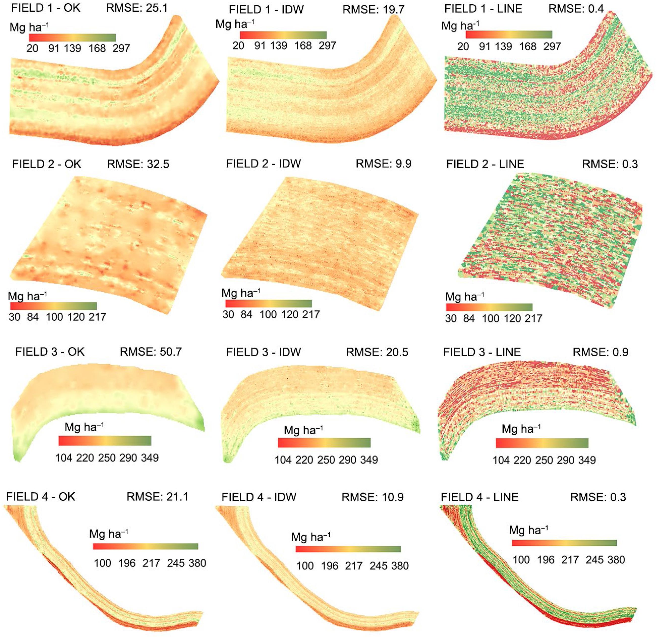
The individual yield lines generated by the extraction method of sugarcane lines and yield estimation by the Voronoi polygon showed that yield variations over short distances were retained (Figure 7). For sugarcane fields, line maps provided detail of yield variations within a sugarcane row. Thus, cropping operations, such as spraying or fertilization, could be carried out with greater accuracy. Surface maps created by OK interpolation tend to smooth out yield variability (Figure 7). The maps generated by OK had higher RMSE values when compared to individual yield lines. This is because both low and high yield variation within the rows frequently disappear when OK is carried out, as regions with low or high yield are not large enough to influence pixel values. OK is known to be a spatial prediction technique that works like a low pass filter through its smoothing effect (Robinson and Metternicht, 2005). This smoothing coupled with the fact that the nugget was greater than zero due to the high randomness of the data, even after excluding outliers, impaired the quality of the interpolation. Surface maps created by IDW interpolation retained minor yield variations over short distances. According to Robinson and Metternicht (2005), IDW introduces substantial variability in the map by virtue of honoring the more extreme valleys and peaks in the harvest data. The IDW interpolator assigns greater weight to the closer yield values than to the farther ones. This is due to a higher power value where the weightings diminish more quickly, return a smaller RMSE in relation to OK (Thylén and Murphy, 1996; Robinson and Metternicht, 2005). Thus, the model retained the yield variations in the data generated by the yield monitor. RMSE values in yield maps generated by IDW and OK demonstrate that with such dense data, surface yield maps are not the approach preferred by management within the same row (Figure 7). Even though the IDW and OK maps show the regions of both low and high yield potential, the OK maps have RMSE variations in relation to the yield average of 20, 33, 23 and 8 % and the IDW maps of 15, 11, 10 and 4 % to fields 1, 2, 3 and 4, respectively. This demonstrates that OK and IDW interpolation methods generate unreliable sugarcane yield maps, which inhibits the use of this site-specific tool in the management of sugarcane unlike individual yield lines, which present a low number of variation errors (an average of 0.3 %) offering high reliability for use in site-specific management, row by row.

Figure 7
Sugarcane yield maps created by ordinary kriging (OK), inverse distance weighting (IDW) and sugarcane lines from cleaning data sets of the four fields. RMSE = root mean square error.

Conclusions

Sugarcane yield data collected along a single or double row have the ability to provide substantial information to the farmer for better field management. Unfortunately, during the process of collecting the yield data, errors occur that are generally associated with the equipment used to obtain them and they have to be identified and removed. This study showed these data can be easily removed by a simple cleaning process of global and anisotropic filtering within a single sugarcane row. In the geostatistical analysis, it was observed that, even after the elimination of data uncertainty, there is a great variation in yield between the adjacent rows, and that this variation is much smaller within a single row. Moreover, frequency data recording influences the yield variability within the row. In this study, the frequency of 2 Hz identified and characterized small yield variations within sugarcane rows whereas frequencies of 0.2 and 0.1 Hz resulted in loss of information on within row yield variability. Therefore, the highest possible frequency of data acquisition by the monitor is recommended. The accuracy assessment of the mapping techniques by the RMSE indicates that the difference between the RMSE, given the IDW and OK techniques. is large enough to suggest the use of an individual yield line map. In this study, individual yield line mapping saved information in the data generated by the yield monitor engendering useful information for row site-specific management. On the other hand, IDW and OK interpolation methods to generate surface maps omitted information over short distances within the rows thereby compromising the quality of high-resolution maps.

References

• Amaral, L.R.; Trevisan, R.G.; Molin, J.P. 2018. Canopy sensor placement for variable-rate nitrogen application in sugarcane fields. Precision Agriculture 19: 147-160.
• Blackmore, B.S.; Moore, M. 1999. Remedial correction of yield map data. Precision Agriculture 1: 53–66.
• Cambardella, C.A.; Moorman, T.B.; Nowak, J.M.; Parkin, T.B.; Karlen, D.L.; Turco, R. F.; Konopka, A.E. 1994. Field-scale variability of soil properties in central Iowa soils. Soil Science Society of America Journal 58: 1501-1511.
• Driemeier, C.; Ling, L.Y.; Sanches, G.M.; Pontes, A.O.; Magalhães, P.S.G.; Ferreira, J. E. 2016. A computational environment to support research in sugarcane agriculture. Computers and Electronics in Agriculture 130: 13-19.
• Fernandes, J.L.; Ebecken, N.F.F.; Esquerdo, J.C.D.M. 2017. Sugarcane yield prediction in Brazil using NDVI time series and neural networks ensemble. International Journal of Remote Sensing 38: 4631-4644.
• Griffin, T.W.; Shockley, J.M.; Mark, T.B. 2018. Economics of precision farming. Precision Agriculture Basics 1: 221-230.
• Isaaks, E.H.; Srivastava, R.M. 1989. An Introduction to Applied Geostatistics. Oxford University Press, New York, NY, USA.
• Jensen, T.A.; Baillie, C.; Bramley, R.G.V.; Panitz, J.H. 2013. An assessment of sugarcane yield monitoring concepts and techniques from commercial yield monitoring systems. International Sugar Journal 115: 53-57.
• Jin, J.; Tang, L. 2010. Optimal coverage path planning for arable farming on 2D surfaces. Transactions of the ASABE 53: 283-295.
• Leroux, C.; Jones, H.; Clenet, A.; Dreux, B.; Becu, M.; Tisseyre, B. 2018. A general method to filter out defective spatial observations from yield mapping data sets. Precision Agriculture 19: 789–808.
• Lyle, G.; Bryan, B.; Ostendorf, B. 2014. Post-processing methods to eliminate erroneous grain yield measurements: review and directions for future development. Precision Agriculture 15: 377–402.
• Mailander, M.; Benjamin, C.; Price, R.; Hall, S. 2010. Sugar cane yield monitoring system. Applied Engineering in Agriculture 26: 965-969.
• Menegatti, L.A.A.; Molin, J.P. 2004. Removal of errors in yield maps through raw data filtering. Revista Brasileira de Engenharia Agrícola e Ambiental 8: 126-134.
• Price, R.R.; Johnson, R.M.; Viator, R.P. 2017. An overhead optical yield monitor for a sugarcane harvester based on two optical distance sensors mounted above the loading elevator. Applied Engineering in Agriculture 33: 687–693.
• QGIS Development Team. 2018. QGIS geographic information system: open source geospatial foundation project. Available at: http://www.qgis.org [Accessed July 10, 2018]
  » http://www.qgis.org
• Ribeiro Júnior, P.P.; Diggle, P.P. 2001. GeoR: a package for geostatistical analysis. R - News 1: 15-18.
• Robinson, T. P.; Metternicht, G. 2006. Testing the performance of spatial interpolation techniques for mapping soil properties. Computers and Electronics in Agriculture 50: 97-108.
• Robinson, T.P.; Metternicht, G. 2005. Comparing the performance of techniques to improve the quality of yield maps. Agricultural Systems 85: 19-41.
• Spekken, M.; Anselmi, A.A.; Molin, J.P. 2013. A simple method for filtering spatial data. p. 259–266. In: Stafford, J.V., ed. Precision agriculture ´13. Wageningen Academic Publishers, Wageningen, The Netherlands. Doi: https://doi.org/10.3920/978-90-8686-778-3_30
  » https://doi.org/10.3920/978-90-8686-778-3_30
• Stolf, R. 1986. Methodology for evaluating skips in sugarcane rows = Metodologia de avaliação de falhas nas linhas de cana-de-açúcar. STAB 4: 22-36 (in Portuguese).
• Sudduth, K.; Drummond, S.T. 2007. Yield editor: software for removing errors from crop yield maps. Agronomy Journal 99: 1471-1482.
• Thylén, L.; Murphy, D.P.L. 1996. The control of errors in momentary yield data from combine harvesters. Journal of Agricultural Engineering Research 64: 271–278.
• Tukey, J.W. 1977. Exploratory Data Analysis. Menlo Park, CA, USA.
• Vega, A.; Córdoba, M.; Castro-Franco, M.; Balzarini, M. 2019. Protocol for automating error removal from yield maps. Precision Agriculture 21: 1-15.
• Vieira, S.; Hatfield, J.; Nielsen, D.; Biggar, J. 1983. Geostatistical theory and application to variability of some agronomical properties. Hilgardia 51: 1-75.

Edited by

Edited by: Paulo Cesar Sentelhas

Publication Dates

• Publication in this collection
  20 Dec 2019
• Date of issue
  2020

History

• Received
  23 Nov 2018
• Accepted
  06 May 2019