
ABSTRACT
Proposing technological innovations in the investigation of the structure and behaviour of wood is important to optimize its use. The assimilation of methods diffused in other areas, such as particle image velocimetry (PIV), can allow a rich range of information for different aspects. The aim of this study was to estimate the Young’s modulus using the PIV technique, independently of the wood density. The Young modulus value was obtained by universal testing machine, transversal vibration and PIV technique. Cedrela spp. and Eucalyptus cloeziana wood specimens were analyzed and their Young modulus were compared and correlated. The PIV technique presented mean Young’s modulus values statistically equal to those of the universal testing machine. The standard error of prediction from PIV approach was 0.46 and 0.97 GPa for Young’s modulus estimates for Cedrela spp. and Eucalyptus cloeziana wood, respectively.
Keywords:
PIV; Modulus of elasticity; Solid mechanics; Measure techniques
INTRODUCTION
Wood is a versatile material whose mechanical properties are crucial to its most diverse uses. When using a wood, it is necessary to understand its anisotropy, which represents a different behaviour as a function of its axes, when submitted to efforts (Panshin and Zeeuw, 1980PANSHIN, A. J.; ZEEUW, C. Textbook of wood technology. McGraw-Hill Book Co,1980. 722p.; Kretschmann, 2010KRETSCHMANN, D. Mechanical properties of wood. In: Forest Products Laboratory Wood handbook: wood as an engineering material. Department of Agriculture, Forest Service, Forest Products Laboratory, 2010. p. 5-46.). Therefore, once the material is known, it is possible to make the best use of it and presume its behaviour under service.
Assays to characterize the mechanical behavior of wood may be performed in a conventional manner using the universal testing machine according to D143 (American society for testing and materials - ASTM, 1994AMERICAN SOCIETY FOR TESTING AND MATERIALS. Standard methods of testing small clear specimens of timber. Philadelphia, PA: ASTM D143, 1994, 50p.) or other standards. This method already consolidated (American society for testing and materials - ASTM, 1994; Kretschmann, 2010KRETSCHMANN, D. Mechanical properties of wood. In: Forest Products Laboratory Wood handbook: wood as an engineering material. Department of Agriculture, Forest Service, Forest Products Laboratory, 2010. p. 5-46.; Associação Brasileira de Normas Técnicas - ABNT, 2011ASSOCIAÇÃO BRASILEIRA DE NORMAS TÉCNICAS. Projeto de estruturas de madeira. Rio de Janeiro, RJ: NBR 7190, 2011, 50p.), is widely used in scientific research. However, these tests require preparation of a large number of test specimens, in addition to a long time to acquire the data. In contrast, non-destructive methodologies perform tests without modifying the structure of the material, allowing its use after the test, seeking to make them more instinctive in obtaining data quickly and directly. Non-destructive methods are already widely used to characterize different materials like wood, fibers, composites, concrete, and aluminum, for example (Carrillo et al., 2019CARRILLO, J., RAMIREZ, J., & LIZARAZO-MARRIAGA, J. Modulus of elasticity and Poisson’s ratio of fiber-reinforced concrete in Colombia from ultrasonic pulse velocities. Journal of Building Engineering, v.23, p.18-26, 2019.; Ettelaei et al., 2019ETTELAEI, A., LAYEGHI, M., HOSSEINABADI, H. Z., & EBRAHIMI, G. Prediction of modulus of elasticity of poplar wood using ultrasonic technique by applying empirical correction factors. Measurement, v.135, p.392-399, 2019.; Osuna-Sequera et at., 2019). So, it is important that new, more specific techniques emerge for wood in different types of loads. Transversal vibration is a non-destructive technique for characterization of materials that use natural vibration frequencies emitted as an acoustic response after a short-term impact (Sharp, 1985SHARP, D.J. Nondestructive testing techniques for manufacturing LVL and predicting performance. In: Proceedings 5th nondestructive testing of wood symposium. Washington State University, 1985. p. 99-108.; Ross, 2015ROSS, R. J. (Ed.). Nondestructive evaluation of wood. Government Printing Office, 2015. 169p.). Ponneth et al. (2014PONNETH, D., VASU, A. E., EASWARAN, J. C., MOHANDASS, A., & CHAUHAN, S. S. Destructive and non-destructive evaluation of seven hardwoods and analysis of data correlation. Holzforschung, v.68, n.8, p.951-956, 2014.) in their work attested the reliability of non-destructive methods to obtain Young´s modulus.
In search of new ways of studying and understanding the behavior of wood, methodologies used in other areas can be adapted. In this sense, the PIV technique, which emerged in the study of gases (Adrian, 1984ADRIAN, R. J. Twenty years of particle image velocimetry. Experiments in fluids, v.39, n.2, p.159-169, 2005.), has been adapted for solid materials. The technique consists of the spatial correlation of the displacement of particles in successive images. The principle of PIV technique is to obtain the deformation from the displacement of points allocated on the surface of the material under study, which can be applied for determination of mechanical properties. The deformation of the material in use is an important source of information about the material and its relation to the environment to which it is exposed (Willert and Gharib, 1991WILLERT, C. E.; GHARIB, M. Digital particle image velocimetry. Experiments in fluids , v. 10, n. 4, p. 181-193, 1991.).
Optical techniques, such as the PIV technique, allow the extraction of quantitative and qualitative information, providing rich insight into the material and the phenomenon observed (Raffel et al., 1998RAFFEL, M.; WILLERT, C.; KOMPENHANS, J. Particle Image Velocimetry - A Practical Guide. Springer-Verlag, 1998. 267p.). Particle image velocimetry allows the deformation of the wood to be determined considering its heterogeneity and the location in the image to be monitored can be chosen according to the criteria of interest. When adapted from studies in fluids and gases to the study of solid materials, the PIV technique needs other types of particles as markers (Pereira et al., 2018PEREIRA, R. A., GOMES, F. C., BRAGA JÚNIOR, R. A., & RIVERA, F. P. Analysis of elasticity in woods submitted to the static bending test using the particle image velocimetry (piv) technique. Engenharia Agrícola, v.38, n.2, p.159-165, 2018.).
Magalhães et al. (2015MAGALHÃES, R.R., BRAGA JR., R.A., AND BARBOSA, B.H.G. Young׳s Modulus evaluation using Particle Image Velocimetry and Finite Element Inverse Analysis. Optics and Lasers in Engineering, v.70, p.33-37, 2015.) monitored deformations in a steel beam (ASTM A36 cantilever type). Whose particles were considered as the points that arise when illuminating the surface with a laser. The PIV technique was used, by means of successive images, to obtain the deformation values of the material. With the deformation and numerical model data with the particle swarm algorithm optimization, the authors calculated the Young’s Modulus. Souza et al. (2014SOUZA, M. T., ELLEM, W. N. F., BRAGA, A. R., BARBOSA, C. H., LIMA, T. J. Non-destructive technology associating PIV and Sunset laser to create wood deformation maps and predict failure. Biosystems Engineering, v. 126, p. 109-116, 2014.) illuminated the wood surface with a sunset laser and used the irregularities of the planed surface to mark the particles to be monitored by the PIV technique. Braga Júnior et al. (2015BRAGA JÚNIOR, R. A., MAGALHÃES, R. R, MELO, P. R. & GOMES, V. J. Maps of deformations in a cantilever beam using particle image velocimetry (PIV) and speckle patterns. Revista Escola de Minas, Ouro Preto, v. 68, n. 3, p. 273-278, 2015.) used a laser to illuminate the surface of steel beams and observe particles during static bending test. Photographs were taken and analyzed by the PIV technique, generating a vector map with the deformation. The authors developed the vector map of the deformation of the wood submitted to the load in the static bending test using the universal testing machine and followed the deformation in the elastic phase, predicting the disruption in a qualitative way. Pereira et al. (2018PEREIRA, R. A., GOMES, F. C., BRAGA JÚNIOR, R. A., & RIVERA, F. P. Analysis of elasticity in woods submitted to the static bending test using the particle image velocimetry (piv) technique. Engenharia Agrícola, v.38, n.2, p.159-165, 2018.) proposed the use of ink dots for random marking of particles on the face of the static bending test specimens. These particles were photographed during the mechanical test. The author also proposed an algorithm to analyze the successive images taking into consideration parameters programmable according to the image to be analyzed. This new methodology allows the algorithm to be fed with assay information and to provide the deformation occurred (Pereira, 2018). Pereira et al. (2019) have successfully applied PIV on specimens of Pinus oocarpa and Eucalyptus grandis wood and also in plywood panels, laminated veneer lumber and oriented strand boards.
The PIV technique does not cause any type of alteration in the study material and can be classified as non-destructive, which makes it of interest for the characterization of materials in service, for example. Its execution is simple and with minimal use of materials allowing it to be conducted in the field. The aim of this study was estimating of Young’s modulus using the PIV technique and test the precision of the its results.
MATERIAL AND METHODS
Material
Timber from Cedrela spp. and Eucalyptus cloeziana, which presented basic densities of 0.260 and 0.680 g.cm-3, respectively, was used. Radial boards were processed to produce 50 flexural test specimens measuring 25 x 25 x 410 mm according to D143 (ASTM, 1994). The specimens were stored in an acclimatization chamber [T = 20 ± 3 oC and UR = 60 ± 5 %], to stabilize the humidity by 12 %.
Transversal Vibration
Using the Sonelastic® transversal vibration equipment, the values of the dynamic Young’s Modulus were obtained after the impact of the metal rod on the specimens. The equipment requests input information about the sample and after vibration on the material is calculated the Young’s Modulus using Equation 1 (ATCP, 2015). In which: Etv: Young’s Modulus (Pa); m: sample weight (g); L: sample length (mm); b: sample width (mm); t: sample thickness (mm); ff: fundamental frequency for the sample in flexional mode (Hz); T1: correction factor.
The test specimens were then subjected to the static bending test in a universal testing machine (EMIC, DL 30 T), according to standard D143 (ASTM, 1994). From the force-by-strain plots, Young’s Modulus values were determined.
Universal Testing Machine and PIV
Concurrently with the static bending tests, for the application of the PIV technique, the specimens were marked on their tangential face with random particles (points) of approximately 0.05 mm2. During the static bending tests (American Society for Testing and Material, 1994), the specimens were photographed by a digital camera (Sony 33). The images were captured every 30 seconds from the beginning of the test until the moment before the specimen ruptured (Figure 1 -b).
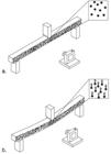
Experiment setup: a-Specimen at the beginning of the test; b -Specimen at the end of the test - highlight of the region of interest and the relative movement of points.
The camera remained static during tests and was triggered by remote control. The images were processed in free software (Image J), in order to have scale and extension compatible with the PIV algorithm. The PIV algorithm was modified to meet the specificities of the static bending test as well as the calculation of the Young’s Modulus. The PIV algorithm tracks the points on the surface of the test material in consecutive images and calculates the displacement (deformation) during the loading phase, which allowed the calculation of the Young’s Modulus. The images from each assay were loaded into the GNU Octave free software and then processed by the PIV algorithm. In the initial image (time = 0 and load = 0) three reference points were selected, which were tracked in each image captured during the test, following the displacement of the particles marked within previously defined regions of analysis. After processing each group of images, the particle image velocimetry deformation reading algorithm provided graphs related to the horizontal and vertical displacement, representing the value of deformation in the static bending test. The graphs allow the evaluation of the accuracy of the displacement values found and if they are reliable. The algorithm also graphically demonstrates if the regions selected in the analysis of the image sequences present a point pattern or markers suitable for the PIV (quality test) technique.
Calculation the Young’s modulus
With the values of deformation calculated by the PIV algorithm and the load values obtained from universal testing machine, the Young’s Modulus was obtained according to Associação Brasileira de Normas Técnicas - ABNT (2011) in order to satisfy Equation 2. In which: Eutm: Young’s Modulus; F: force (N); V: deformation (m); L: free range (m); b: sample width (m); h: sample thickness (m).
Data analysis
The experiment was conducted in a completely randomized design and the data were analyzed with the Rstudio free software. Analyzes of data normality and variance (ANOVA) were performed, at 1 % significance, for the hypothesis of a difference between methods. If significant, multiple comparisons of the means by the Tukey test, at 1 % of significance were performed.
RESULTS AND DISCUSSION
The descriptive statistics
For Young’s Modulus values of Cedrela spp. and Eucalyptus cloeziana are shown in Table 1. The species for Cedrela spp. presented the means values of Young´s modulus approximate.
The summary of the variance analysis of the Young’s Modulus of the Cedrela spp. and Eucalyptus cloeziana. For the wood of Cedrela spp. there was no significant difference. The wood of E. cloeziana had a difference between methods and therefore, a multiple comparison of means was made via Tukey’s test (Table 1). Statistical similarity was found between the Young’s Modulus values estimated by particle image velocimetry and the universal testing machine, both of which were different from the transversal vibration method. Fonseca et al. (2016FONSECA, C. S.; SILVA, T. D., ;SILVA, M. F.; OLIVEIRA, I. D. C.; MENDES, R. F.; HEIN, P. R. G.; TONOLI, G. H. D. Micro/nanofibrilas celulósicas de Eucalyptus em fibrocimentos extrudados. Cerne, v.22, n.1, p.59-68, 2016.) have had difficulty relating to Young’s Modulus found by the transversal vibration and the universal machine. For Cedrela spp., low-density wood (ρ=0.260 g.cm-3), there was no difference between the methods. However, for Eucalyptus cloeziana, high density (ρ =0.680 g.cm-3), whose Young’s Modulus values are higher, there was a significant difference between methods. To better understand this behaviour, the Tukey test was performed with the Eucalyptus cloeziana species, and it was verified that the transversal vibration method differed from the others.
For the Eucalyptus cloeziana, through the multiple comparisons of the means we observed that the PIV was statistically equal to the universal testing machine, this is a positive point since this is the method used as a reference. PIV presented statistically different Young’s Modulus values from those presented by transversal vibration. In transversal vibration the Young’s Modulus calculation uses the rigidity of the material, which is obtained as an acoustic response; in contrast, the PIV technique analyzes the displacement (deformation) at each image. In this way, the values obtained, although close, are different interpretations of the Young’s Modulus. This result is consistent with the literature data for the conventional method using the universal testing machine since wood with lower densities tends to have lower Young’s Modulus values than higher density wood.
Comparative analysis between methods
By means of Pearson correlation (Table 2), is observed that the modulus of elasticity obtained by PIV technique had a strong and positive correlation with the other methods.
Pearson correlation between the values of Young’s modulus obtained by the three methods. Correlations for Eucalyptus wood are presented above diagonal while correlations for Cedrela wood are below diagonal.
The coefficients of determination between the PIV and the universal testing machine were high (R2 = 0.72 for Cedrela spp. and R2 = 0.75 for Eucalyptus cloeziana) for the two species. These values indicate that there is a correlation between the techniques. The standard error (SEE) of the adjusted regression for the Cedrela spp. species was 0.46 GPa and for Eucalyptus cloeziana was 0.97 GPa (Figure 2).

Correlation between the Young’s Modulus (GPa) obtained by methods. (a) and (b) Young’s Modulus for Cedrela spp. and (c) and (d) for Eucalyptus cloeziana.
For the models adjusted between PIV and transversal vibration, the same did not occur. The regression coefficient for the Eucalyptus cloeziana was 0.65 and a lower value for Cedrela spp. was 0.14. Observing the graph (Figure 2) is perceptible that the s values have dispersed away from the line. The error of the model (1.23 for Cedrela spp. and 1.16 for Eucalyptus cloeziana) above 1 confirms that the adjustment was not so suitable among the techniques.
CONCLUSION
It was possible to calculate Young´s modulus of wood specimens based on PIV technique. The modulus of elasticity values estimated by PIV were statistically similar to the reference value obtained by the universal testing machine. The plot of values obtained by PIV technique and universal testing machine yielded coefficient of determination of 0.72 for Cedrela spp. and 0.75 for Eucalyptus cloeziana. The standard error of estimation of the PIV was low (SEE = 0.46 GPa for Cedrela and SEE = 0.97 GPa for Eucalyptus) showing good accuracy to estimate values.
REFERENCES
- ADRIAN, R. J. Twenty years of particle image velocimetry. Experiments in fluids, v.39, n.2, p.159-169, 2005.
- AMERICAN SOCIETY FOR TESTING AND MATERIALS. Standard methods of testing small clear specimens of timber Philadelphia, PA: ASTM D143, 1994, 50p.
- ASSOCIAÇÃO BRASILEIRA DE NORMAS TÉCNICAS. Projeto de estruturas de madeira Rio de Janeiro, RJ: NBR 7190, 2011, 50p.
- ATCP ENGENHARIA E INDÚSTRIA. Manual de instalação e operação software Sonelastic 3.0. ATCP, 2015. 88p.
- BRAGA JÚNIOR, R. A., MAGALHÃES, R. R, MELO, P. R. & GOMES, V. J. Maps of deformations in a cantilever beam using particle image velocimetry (PIV) and speckle patterns. Revista Escola de Minas, Ouro Preto, v. 68, n. 3, p. 273-278, 2015.
- CARRILLO, J., RAMIREZ, J., & LIZARAZO-MARRIAGA, J. Modulus of elasticity and Poisson’s ratio of fiber-reinforced concrete in Colombia from ultrasonic pulse velocities. Journal of Building Engineering, v.23, p.18-26, 2019.
- ETTELAEI, A., LAYEGHI, M., HOSSEINABADI, H. Z., & EBRAHIMI, G. Prediction of modulus of elasticity of poplar wood using ultrasonic technique by applying empirical correction factors. Measurement, v.135, p.392-399, 2019.
- FONSECA, C. S.; SILVA, T. D., ;SILVA, M. F.; OLIVEIRA, I. D. C.; MENDES, R. F.; HEIN, P. R. G.; TONOLI, G. H. D. Micro/nanofibrilas celulósicas de Eucalyptus em fibrocimentos extrudados. Cerne, v.22, n.1, p.59-68, 2016.
- KRETSCHMANN, D. Mechanical properties of wood. In: Forest Products Laboratory Wood handbook: wood as an engineering material. Department of Agriculture, Forest Service, Forest Products Laboratory, 2010. p. 5-46.
- MAGALHÃES, R.R., BRAGA JR., R.A., AND BARBOSA, B.H.G. Young׳s Modulus evaluation using Particle Image Velocimetry and Finite Element Inverse Analysis. Optics and Lasers in Engineering, v.70, p.33-37, 2015.
- OSUNA-SEQUERA, C., LLANA, D. F., ESTEBAN, M., & ARRIAGA, F. Improving density estimation in large cross-section timber from existing structures optimizing the number of non-destructive measurements. Construction and Building Materials, v.211, p.199-206, 2019.
- PANSHIN, A. J.; ZEEUW, C. Textbook of wood technology. McGraw-Hill Book Co,1980. 722p.
- PEREIRA, R. A., GOMES, F. C., BRAGA JÚNIOR, R. A., & RIVERA, F. P. Analysis of elasticity in woods submitted to the static bending test using the particle image velocimetry (piv) technique. Engenharia Agrícola, v.38, n.2, p.159-165, 2018.
- PEREIRA, R. A., GOMES, F. C., BRAGA JÚNIOR, R. A., & RIVERA, F. P. Displacement measurement in sawn wood and wood panel beams using particle image velocimetry. Cerne , v.25, n.1, p.110-118, 2019.
- PONNETH, D., VASU, A. E., EASWARAN, J. C., MOHANDASS, A., & CHAUHAN, S. S. Destructive and non-destructive evaluation of seven hardwoods and analysis of data correlation. Holzforschung, v.68, n.8, p.951-956, 2014.
- RAFFEL, M.; WILLERT, C.; KOMPENHANS, J. Particle Image Velocimetry - A Practical Guide. Springer-Verlag, 1998. 267p.
- ROSS, R. J. (Ed.). Nondestructive evaluation of wood. Government Printing Office, 2015. 169p.
- SHARP, D.J. Nondestructive testing techniques for manufacturing LVL and predicting performance. In: Proceedings 5th nondestructive testing of wood symposium. Washington State University, 1985. p. 99-108.
- SOUZA, M. T., ELLEM, W. N. F., BRAGA, A. R., BARBOSA, C. H., LIMA, T. J. Non-destructive technology associating PIV and Sunset laser to create wood deformation maps and predict failure. Biosystems Engineering, v. 126, p. 109-116, 2014.
- WILLERT, C. E.; GHARIB, M. Digital particle image velocimetry. Experiments in fluids , v. 10, n. 4, p. 181-193, 1991.
HIGHLIGHTS
-
It was possible to obtain the Young’s modulus using Particle Image Velocimetry.
-
The estimates of MOE by PIV presented SEE ranging from 0.46 to 0.97 GPa.
-
PIV applied in viscoelastic materials is recent and innovative.
-
MOE values estimated by PIV technique do not differ from those obtained by universal testing machine.
Publication Dates
-
Publication in this collection
09 Sept 2019 -
Date of issue
Apr-Jun 2019
History
-
Received
20 Mar 2019 -
Accepted
24 May 2019


