A BRANCH AND BOUND ALGORITHM FOR FINDING THE POSITIVE INFLUENCE DOMINATING SET ON CHORDAL GRAPHS

ABSTRACT

We address the Positive Influence Dominating Set problem (PIDS), which involves identifying the smallest group of vertices in a given network that maximizes influence throughout the network. Formally, given a graph G = (V, E), representing the network, we look for a subset of vertices P ⊆ V such that each vertex v _i ∈ V \ P has at least ρ deg_G (v _i ) neighbors in P, where deg_G (v _i ) is the degree of v _i , and 0 < ρ < 1. The problem is known to be NP-hard in general graphs and remains NP-hard even when restricted to certain particular classes, such as chordal graphs. In this paper, we develop an exact algorithm based on the Branch and Bound approach for solving PIDS on chordal graphs. The effectiveness of the proposed algorithm is demonstrated through numerical experiments conducted on various randomly generated chordal graphs.

Keywords:
branch and bound; clique decomposition; dominating set; positive influence; chordal graphs; social networks

1 INTRODUCTION

The Positive Influence Dominating Set problem (PIDS) was initially introduced by Wang et al. (2009) to model the spread of influence among individuals in online social networks, addressing certain social challenges. Specifically, they aimed to identify the smallest set of dominant individuals capable of exerting a positive influence on others within the network, with an application to mitigating the issue of excessive drinking on college campuses. Since its introduction, numerous studies have been carried out to address this problem (Borgati, 2006; Zou et al., 2009; Zareie & Sheikhahmadi, 2018; Sun & Ng, 2012; Mbaru & Barnes, 2017; Gursoy & Gunnec, 2018; He et al., 2014; Raghavan & Zhang, 2022). A comprehensive review and classification of various solution approaches proposed in the literature is provided in Bekhti et al. (2025).

The PIDS problem has valuable applications across various domains (Hsu & Park, 2012; Lalou et al., 2025). For example, in the context of a charity event, PIDS can be used to strategically identify key donors who are likely to influence their network, encouraging broader participation and maximizing donations. This approach fosters a larger community of generous contributors, ultimately aiding more people in need. Similarly, in auctions, PIDS can help optimize profits by selecting items that generate the most interest among buyers. Such items are likely to attract higher bids, ensuring maximum sales and broader buyer engagement.

The PIDS problem is APX-hard on general graphs (Wang et al., 2011), which has led to the development of various heuristic approaches that deliver high-quality solutions within reasonable computational times. Wang et al. (2011) introduced the first greedy heuristic for PIDS on general graphs, with a time complexity of O(n ³). This algorithm guarantees an H(∆)-approximation, where H represents the harmonic function, ∆ is the maximum vertex degree, and n is the number of vertices. Subsequently, a more efficient greedy algorithm with O(n ²) complexity was proposed in Raei et al. (2012). Dhawan & Rink (2015) further improved upon these results, presenting an O(n ²)-time algorithm that produces smaller PIDS solutions compared to those of Wang et al. (2011); Raei et al. (2012). Later, Abu-Khzam & Lamaa (2018) designed four heuristics tailored for various online network structures. Their approach iteratively selects vertices based on maximum utility and/or minimum need, balancing the vertex’s potential for positive dominance over its neighbors and the number of neighbors still requiring positive domination. More recently, Bouamama & Blum (2021) proposed a simple greedy algorithm leveraging problem-specific insights, demonstrating superior performance compared to existing heuristics.

In the realm of meta-heuristics, Khomami et al. (2018) developed an automata learning algorithm that selects iteratively the candidate vertices for inclusion in the PIDS, such that each vertex learns how to choose its action during the search process to minimize the constructed solution cardinality. Lin et al. (2018) proposed a memetic approach using tabu search for solution space exploration and genetic operators for solution recombination. Recently, Bekhti et al. (2026) introduced a Local Branching algorithm for the PIDS problem. The proposed approach improved several best-known results on benchmark instances and demonstrated the effectiveness of combining exact and heuristic search strategies for influence maximization.

Several variants of the PIDS problem have been explored in the literature. Wang et al. (2013b) investigated the Weighted Positive Influence Dominating Set problem, proposing two methods for solving it on general graphs. They also introduced a stabilizing algorithm (Wang et al., 2013a) with a time complexity of O(n ²) for general graphs. Du et al. (2019) studied the Connected Positive Influence Dominating Set problem on large-scale graphs, presenting a greedy approach that starts with an initial PIDS solution and employs Steiner trees to enforce connectivity constraints, along with a vertex-removal procedure to eliminate redundancies.

Greetham et al. (2020) addressed the Minimum Weighted Total Positive Influence Dominating Set problem, proposing three solution methods: two greedy techniques and a linear programming-based approximation algorithm. More recently, Yao et al. (2020) examined two variants: the Connected Positive Influence Dominating Set problem and the Partial Positive Influence Dominating Set problem. They proposed greedy algorithms for each variant, achieving H(12) and H(9) approximation guarantees, respectively, on K-regular graphs.

Given the NP-hard nature of the PIDS problem, most related studies, as we can note, emphasize the development of approximation and heuristic approaches that yield reasonably good solutions within practical computational times. However, in certain circumstances, exact methods may be more desirable, despite their higher computational expense, as they guarantee optimal solutions and can sometimes be the best choice. Motivated by this, we focus on exact approaches for solving PIDS. In this paper, we propose a branch and bound-based method to tackle this problem, specifically on one of the most significant classes of graphs, namely the class of chordal graphs.

A graph is called chordal if it contains no induced cycle of length greater than three, i.e., every cycle of length at least four has a chord (an edge connecting two non-consecutive vertices of the cycle). The motivation for considering this class of graphs stems from their significance and flexibility in modeling various real-world networks, particularly those characterized by transitive relationships, captured by the principle “The friend of my friend is also my friend”. These networks typically comprise small, densely connected components in which every element is directly connected to all others within the same component.

The rest of the paper is structured as follows. In Section 2, we formally define the problem. In Section 3, we detail our approach and describe, through detailed examples, different branching and cutting procedures. Section 4 provides the experimental results obtained through performing our approach on different randomly generated chordal graphs.

2 DEFINITIONS AND NOTATIONS

Consider a finite simple undirected graph G = (V, E), such that V is the set of vertices, where |V | = n, and E is the set of edges, where |E| = m. For each v ∈ V , we denote by deg_G (v) the degree of v _i in G, corresponding to the number of edges incident to v, and by N _G (v) the set of vertices in G adjacent to v, i.e. the neighborhood of v in G. Similarly, we denote by N _S (v) the set of vertices in S adjacent to v, and by n _S (v) the cardinality of N _S (v). The needed number of vertices for v to be positively dominated, called the needed degree of v, is denoted by h(v) and is expressed in terms of deg_G (v). We denote by N _G (S), the set of vertices in G adjacent to all the vertices of S. Finally, recall that a clique decomposition of G is a partition of its set of vertices into maximal complete subgraphs. Note that this decomposition is not necessarily unique, since a vertex can belong to several of these cliques, but is assigned to only one.

The minimum Positive Influence Dominating Set problem, PIDS, on G = (V, E) consists of finding the smallest subset of vertices P ⊆ V , such that for each v ∈ V \P, we have |N _G (v) ∩ P| ≥ ρ deg_G (v), for some constant 0 < ρ < 1. The recognition version of PIDS can be formulated as follows:

L-PIDS problem: Minimum Positive Influence Dominating Set problem

• || Input: A graph G = (V, E) representing a network, an integer L, and a ratio ρ, 0 < ρ < 1.

• || Output: Is there a subset P of L vertices such that for each v ∈ V \ P, we have |P ∩ N _G (v)| ≥ ρ deg_G (v) ?

Where ρ is a constant called the Influence Factor that depends on the application at hand, and determines for each vertex v the minimum number of neighbors that must be included in P so that v becomes positively dominated.

A 0-1 programming formulation of the problem (Lin et al., 2018) can be established as follows. Let A = (a _ij )_n×n be the symmetric adjacency matrix of the given graph G, where a _i,j = 1 if (v _i , v _j ) ∈ E otherwise a _i,j = 0. Also, let x _i be a binary variable such that x _i = 1 if v _i ∈ P, x _i = 0 otherwise. We have:

$\left\{\begin{array}{l}\min f\left(x\right)=\sum _{v_i\in V}{x}_i\left(1\right)\\ s.t.\sum _{v_j\in V}{a}_{ij}{x}_j\ge \lceil \rho {\mathrm{deg}}_G\left(v_i\right)\rceil \forall v_i\in V\left(2\right)\\ x_i\in \{0,1\}\forall v_i\in V\left(3\right)\end{array}\right.$

The objective function f(x) minimizes the number of selected vertices and is accomplished by (1). Constraints (2) ensure that vertex v _i has at least ⌈ρ deg_G (v _i )⌉ of its neighbors in the PIDS solution. Constraints (3) provide the domain of the used variables.

3 BRANCH & BOUND APPROACH FOR SOLVING PIDS ON CHORDAL GRAPHS

Throughout the approach explanation, we consider the chordal graph in Figure 1 to illustrate, by detailed examples, each step of the algorithm. The graph is labeled such that each vertex v _i is annotated with label a/b, where a presents the degree of v _i and b represents the needed degree of v _i to be dominated. For example, vertex v ₆ is labeled 5/3, meaning that it has a degree of 5 and requires 3 neighbor vertices in PIDS to be dominated, assuming the default value of ρ = 0.5.

Figure 1
A chordal graph G. For each vertex, label a/b represents the vertex degree, denoted by a, and the needed degree for the vertex to become dominated, denoted by b.

The main idea of our Branch and Bound approach is structured in three primary steps. In the first step, the input graph is partitioned into maximal cliques utilizing the clique decomposition. The vertices are then sorted in a specific order, according to the clique size and vertex degree, to facilitate the incremental construction of the positive dominants set. The remaining two steps correspond to the standard phases of a Branch and Bound algorithm, namely Branching and Evaluation. For each vertex v _i of G, it proceeds to a branching considering the two possible cases, whether or not v _i is in PIDS. Then, it evaluates the solution of the new sub-problem considering v _i by computing the upper and lower bounds. Note that the positive dominant set is built progressively by processing each vertex of G. The last two steps are repeated for every candidate vertex until all vertices have been processed. The following outline summarizes the main steps of the approach; each one will be explained in detail in the subsequent sections.

• - Step 1. Preprocessing. Perform a clique decomposition of the input graph. The vertices are then sorted in ascending order based on both the size of their cliques and their degrees.

• - Step 2. Branching. Use a binary search tree to deal with each candidate vertex of G, considering both cases, whether or not it is in PIDS.

• - Step 3. Evaluation. Compute the upper and lower bounds to evaluate the solution of the new sub-problem considering v _i .

3.1 Chordal graph preprocessing

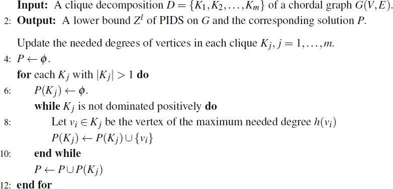
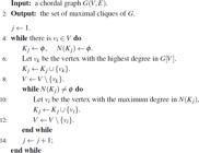
As stated previously, chordal graphs are characterized by small and densely connected components. The first step leverages this property and consists of partitioning the input graph into maximal cliques K _j , j = 1, . . . , m (where m is the number of cliques). We refer to N(K _j ) as the set of neighbors of all vertices included in the clique K _j . This can be done, in polynomial time, using the following algorithm:

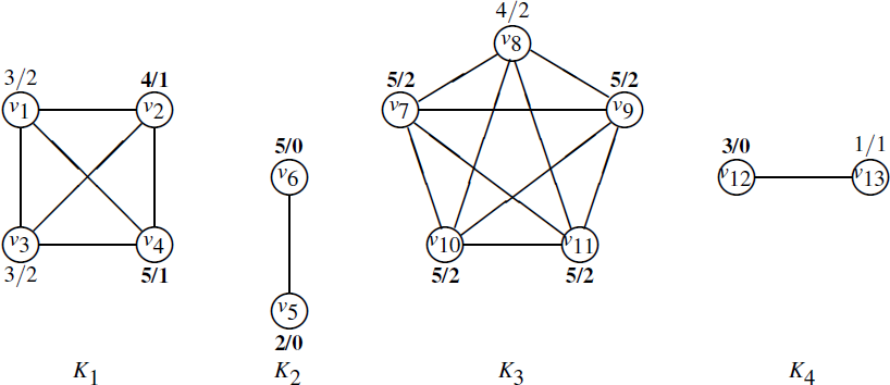
Considering the chordal graph G in Figure 1, Algorithm 1 returns four maximal cliques, namely K ₁ = {v ₁ , v ₂ , v ₃ , v ₄}, K ₂ = {v ₅ , v ₆}, K ₃ = {v ₈ , v ₇ , v ₉ , v ₁₀ , v ₁₁}, and K ₄ = {v ₁₂ , v ₁₃}, as follows (see Figure 2).

Figure 2
The maximal cliques decomposition of the chordal graph G in Figure 1.

Algorithm 1
Graph decomposition on maximal cliques.

The Branch and Bound algorithm greedily constructs the positive dominants set by processing each vertex of G in turn. To enhance the algorithm’s efficiency (see Section 4), vertices are processed in increasing order based on both their clique size and their degree. Specifically, cliques K _j , j = 1, . . . , m, are ordered by size, and within each clique, vertices are further sorted by their degrees. For instance, considering the graph G in Figure 1, the vertices are processed in the following order: {{v ₉ , v ₁₁ , v ₇ , v ₁₀ , v ₈},{v ₄ , v ₂ , v ₁ , v ₃}, {v ₆ , v ₅}, {v ₁₂ , v ₁₃}}.

3.2 Branching

Let P _t denote the current positive influence dominating set being constructed while processing vertex v _i (initially, $P_0=\cancel{0}$), and C _t the set of candidate vertices (initially, C ₀ = V). Note that P _t and C _t are disjoint sets, and their union P _t ∪ C _t represents a feasible solution for PIDS on G at the iteration t. Additionally, let T represent the binary search tree used for branching on each candidate vertex v _i of G, where each node s _t ∈ T corresponds to a candidate vertex v _i (we use ”node” for T and ”vertex” for G). The two cases-whether v _i is included in P _t or not-are represented by the left and right children of s _t , respectively. Figure 3 illustrates the case of handling the first two vertices of G, v ₉ and v ₁₁, from Figure 1 according to the order. The left (resp. right) child of s ₀ corresponds to the case where v ₉ is (resp. is not) included in the current positive influence dominating set P _t .

Figure 3
Branching using a binary search tree - The case of branching on the first vertex in the order v ₉.

For each node s _t , we evaluate whether the current P _t constitutes an optimal and feasible solution for the subgraph induced by the vertices that are neither in P _t nor dominated by P _t .

Adding cuts. The Branch and Bound efficiency can be significantly improved by strategically reducing the search space that cannot contain optimal solutions. In the following, we explain how the added cuts are integrated within the algorithm.

A vertex v _i of clique K _j is referred to as a local positive dominant vertex if it is a positive dominant for vertices within its clique K _j , and is therefore included in P. Conversely, v _i is considered a local dominated vertex if it does not necessarily need to be added to P, as dominants can instead be selected from among its neighbors in K _j . This is the case of v ₈ from K ₃ in Figure 2. Clearly, given an optimal solution P that includes v ₈, a solution as good as P can be obtained by substituting v ₈ with any vertex from {v ₇ , v ₉ , v ₁₀ , v ₁₁}. Consequently, v ₈ is considered as a local dominated vertex, to be excluded from P, while the set {v ₇ , v ₉ , v ₁₀ , v ₁₁} is identified as local positive dominants that are likely contributors to the final solution.

Let $P_{in}^j$ and $P_{out}^j$ denote, respectively, the set of local positive dominants and the set of local dominated vertices in clique K _j . Define $g_j=\{v_i\in K_j:h(v_i)>\lceil \frac{\left|K_j\right|-1}{2}\rceil \}$, the set of vertices in K _j with needed degree strictly greater than $\lceil \frac{\left|K_j\right|-1}{2}\rceil$. Considering the cliques in Figure 2, we have g ₂ = {v ₆} since h(v ₆) = 3 > 1. The subsets $P_{in}^j$ and $P_{out}^j$ for clique K _j are constructed as follows:

Case 1. If $0<\left|g_j\right|<\lceil \frac{\left(\right|K_j|-1)}{2}\rceil$, then vertices in g _j are local positive dominants, and hence placed in $P_{in}^j$. This is the case of K ₁ in Figure 2. We have g ₁ = {v ₄}, and so vertex v ₄, of needed degree h(v ₄) = 3 > 2, is to be added to $P_{in}^1$. Furthermore, two classes of vertices in K _j \ g _j can be distinguished: vertices with degrees equal to |K _j | − 1, and vertices with degrees equal to |K _j |, denoted, hereafter, S and S’, respectively. To better illustrate the different configurations that may arise in this case, Figure 4 depicts the two scenarios corresponding to the sets S and S’.

Figure 4
The illustration of the case where $0<\left|g_j\right|<\lceil \frac{\left(\right|K_j|-1)}{2}\rceil$.

According to the cardinality of S, we have two sub-cases:

• - If $\left|S\right|>\lceil \frac{\left(\right|K_j|-1)}{2}\rceil -\left|g_j\right|$ (see Figure 4 (a)), then we add to $P_{in}^j$ vertices of S’. If the new constructed $P_{in}^j$ fewer elements than $\lceil \frac{\left(\right|K_j|-1)}{2}\rceil$, we complete it by selecting randomly $\lceil \frac{\left(\right|K_j|-1)}{2}\rceil -|g_j\cup S\text{'}|$ vertices from S. The vertices of $S\setminus P_{in}^j$ that are not selected will be positively dominated and, therefore, placed in $P_{out}^j$.

• - If $\left|S\right|\le \lceil \frac{\left(\right|K_j|-1)}{2}\rceil -\left|g_j\right|$ (see Figure 4 (b)), we include the vertices of S in $P_{out}^j$ to be dominated. The algorithm will choose the positive dominants from S’ and combine them with vertices of $P_{in}^j$ to ensure the positive domination of the vertices in $P_{out}^j$.

Case 2. If $\left|g_j\right|\ge \lceil \frac{\left|K_j\right|-1}{2}\rceil$, then vertices in K _j \ g _j are local dominated vertices, and so the algorithm places them in $P_{out}^j$. This is the case of K in Figure 2, where g ₃ = {v ₇ , v ₉ , v ₁₀ , v ₁₁} and so |g ₃| > 2, vertex v ₈ will be added to $P_{out}^3$.

Case 3. If |K _j | ≤ 2, i.e. cliques of size ≤ 2 with pendant vertex, the algorithm places the pendant vertex in $P_{out}^j$ and its exclusive neighbors in $P_{in}^j$. This is the case of clique K ₄, where vertex v ₁₃ will be added to $P_{out}^4$ and its only neighbor, vertex v ₁₂, to $P_{in}^4$. This ensures that the selected neighbors dominate the pendant vertices and actively contribute to the positive domination of their other remaining neighbors. Additionally, if |K _j | = 1, when the clique is an isolated vertex with degree equal to 0, the vertex is also added to $P_{in}^j$ as there is no other vertex that can dominate it positively.

Note that when |g _j | = 0, the clique K _j has no vertex connected to any other clique of graph G. In this case, K _j forms a disconnected component that requires exactly $⌈\frac{\left|K_j\right|-1}{2}⌉$ vertices (see Observation 1).

Lemma 1.$P_{in}={\cup }_{j=1}^m{P}_{in}^j$, where m is the number of cliques, constitutes a suboptimal solution for PIDS on G.

Proof. Let P be a minimum positive influence dominating set for a given chordal graph G = (V, E), with $P\cap P_{in}=\cancel{0}$. We prove that there exists an optimal solution that contains P _in vertices. Let v _i be a vertex where $v_i\in P_{in}^j\cap K_j$ and v _i ∉ P, we have three possible cases:

• - If v _i is an isolated vertex with degree 0, then v _i must be included in P _in . However, since P is a positive influence dominating set of G, it must also include v _i to ensure the positive domination. This leads to a contradiction with the assumption that $P\cap P_{in}=\cancel{0}$.

• - If v _i is a neighbor of a pendant vertex v _k , then v _i is included in $P_{in}^j$. Given the assumption that $P\cap P_{in}=\cancel{0}$, it follows that v _k must belong to P to be positively dominated. By replacing v _k with v _i in P, we can verify that (P \{v _k })∪{v _i } also forms a minimum positive influence dominating set, since v _k is positively dominated by v _i , and its sole neighbor v _i is included in the newly formed P, i.e. v _i ∈ P.

• - For the last case, if v _i is added to P _in , it means that v _i is selected for some maximal clique K _j with $\left|g_j\right|<\lceil \frac{\left|K_j\right|-1}{2}\rceil$. This implies either that v _i is added to $P_{in}^j$ because its degree satisfies ${\mathrm{deg}}_G\left(v_i\right)>\left|K_j\right|$, or because its degree falls within the range $\left|K_j\right|-1\le {\mathrm{deg}}_G\left(v_i\right)\le \left|K_j\right|$.

• - For the last case, if v _i is added to P _in , it means that v _i is selected for some maximal clique K _j with $\left|g_j\right|<\lceil \frac{\left|K_j\right|-1}{2}\rceil$. This implies either that v _i is added to $P_{in}^j$ because its degree satisfies ${\mathrm{deg}}_G\left(v_i\right)>\left|K_j\right|$, or because its degree falls within the range $\left|K_j\right|-1\le {\mathrm{deg}}_G\left(v_i\right)\le \left|K_j\right|$. Since $\left|g_j\right|<\lceil \frac{\left|K_j\right|-1}{2}\rceil$, less than $\lceil \frac{\left|K_j\right|-1}{2}\rceil$ vertices of the clique K _j have neighbors outside K _j . Consequently, at least |K _j | − |g _j | vertices in K _j have all their neighbors entirely within the clique. It follows that $|P\cap K_j|\ge \lceil \frac{\left|K_j\right|-1}{2}\rceil$. In other words, if the number of vertices in K _j with neighbors outside the clique is greater than $2·\lceil \frac{\left|K_j\right|-1}{2}\rceil$ (i.e., ${\mathrm{deg}}_G\left(v_i\right)>\left|K_j\right|-1$) and $\left|g_j\right|<\lceil \frac{\left|K_j\right|-1}{2}\rceil$, then only a few vertices of K _j have external neighbors and many vertices have no neighbors outside the clique. Since each vertex inside the clique requires at least $\lceil \frac{\left|K_j\right|-1}{2}\rceil$ neighbors within the clique for positive domination (according to Observation 1), it follows that $|P\cap K_j|\ge \lceil \frac{\left|K_j\right|-1}{2}\rceil$.

• In an optimal way, we first select vertices from g _j because they contribute to dominating both the clique and external neighbors, and then we arbitrarily add enough vertices from K _j to reach the required number $\lceil \frac{\left|K_j\right|-1}{2}\rceil$, ensuring the clique is positively dominated.

• Since the number of vertices having all their neighbors within clique K _j is greater than $\lceil \frac{\left|K_j\right|-1}{2}\rceil$, it follows that $|P\cap K_j|\ge \lceil \frac{\left|K_j\right|-1}{2}\rceil$.

• Furthermore, under the assumption $P\cap P_{in}^j=\cancel{0}$, the vertices in P ∩ K _j have all their neighbors within K _j . By replacing each vertex in P ∩ K _j with a corresponding vertex from P _in ∩ K _j , we obtain a positive influence dominating set (PIDS) with the same cardinality. The removed vertices in the new PIDS have at least half of their neighbors included in the new PIDS, ensuring they are positively dominated. □

Vertices in P _in should result in a cut on the left child branch of the search tree. Similarly, vertices in P _out , being dominated by other vertices, should also lead to a cut on the right child branch, i.e., no exploration of the right children occurs during the search process. Note that vertices in P _in ∪ P _out are removed from the list of candidate vertices considered by the algorithm. Furthermore, the list of candidate vertices is updated after processing each vertex. If a vertex v _i is positively dominated, and its neighbors are either positively dominated as well or have already been visited before v _i , i.e., v _i ’s neighbors appear earlier in the list of candidate vertices, then the algorithm branches on the next vertex, thereby excluding v _i .

3.3 Evaluation

The evaluation of a solution involves computing the lower and upper bounds of the sub-problem at each iteration as follows. Let Z ^u and Z ^l be the upper and lower bounds for the input graph G.

3.3.1 Upper bound

To determine an upper bound for the problem, we solve the PIDS for each clique K _j , j = 1, . . . , m, of G, independently. The upper bound is then defined as the union of the PIDS obtained for all the cliques. Note that vertices are processed in increasing order, ensuring that the resulting positive dominants are the vertices with the maximum degrees within each clique K _j .

Observation 1.The cardinality of the minimum positive dominating set on a complete graph K_nis$\lceil \frac{n-1}{2}\rceil$.

Based on this observation, we have the upper bound of the chordal graph established by the following proposition.

Proposition 1.The upper bound of the chordal graph is$Z^u=\sum _{j=1}^m\lceil \frac{\left|K_j\right|-1}{2}\rceil$.

We can use a simple greedy heuristic that progressively adds to the positive dominant set the vertex with the highest degree in the graph induced by the set of vertices not yet dominated until we obtain a PIDS. This returns a feasible solution for the input graph.

3.3.2 Lower bound

To compute a lower bound for the problem, we proceed as follows. First, we identify the edges removed by the clique decomposition of the input graph G, i.e., the edges connecting the maximal cliques. Next, for each vertex incident to a removed edge, we consider the other endpoint of the edge as a positive dominant and update the vertex’s needed degree accordingly. Considering the clique decomposition of the graph G in Figure 1, the updated needed degree of each vertex is illustrated in Figure 5. For example, vertex v ₂ is incident to a single removed edge (v ₂ , v ₆), so its updated needed degree becomes h(v ₂) = 1, reduced from 2 before the update. The lower bound is then defined as the union of the suboptimal solutions of PIDS obtained for all cliques, considering the updated degrees (see Algorithm 2).

Figure 5
The updated needed degrees (in bold) of vertices after the clique decomposition.

Algorithm 2
Computing a lower bound of PIDS after updating the vertex needed degrees.

Algorithm 2 constructs first a PIDS for each clique K _j , after updating the needed degrees of the vertices, and then defines the lower bound for the corresponding chordal graph as the union of the PIDS of all cliques. For the graph in Figure 2, it returns as positive dominants P(K ₁) = {v ₁ , v ₃}, P(K ₃) = {v ₇ , v ₁₁} and P(K ₄) = {v ₁₃} for, respectively, cliques K ₁, K ₃ and K ₄.

Lemma 2.P(K_j ) is a minimum positive influence dominating set of clique K _j after updating the needed degrees of the vertices.

Proof. Let P(K _j ) = {v ₁ , v ₂ , . . . , v _i , . . . , v _k } be the minimal positive influence dominating set for the clique K _j returned by Algorithm 2 after updating the needed degrees. Suppose there exists a positive dominating set P’ of K _j with cardinality smaller than that of P(K _j ). This implies that there exists at least one vertex v _i ∈ P(K _j ) such that v _i ∉ P’. For each vertex v _k ∈ P’, if v _k ∉ P(K _j ) we replace v _k with a vertex from P(K _j )\{v _i }. As K _j is a clique, the vertex replacing v _k is adjacent to all vertices of K _j . Moreover, after updating the needed degrees, replacing v _k by a vertex from P(K _j ) does not increase the number of needed positive dominants for any vertex of the clique. In particular, vertices with h(v) = 0 remain dominated, while vertices with h(v) > 0 are dominated at least as effectively as before. By doing so, we obtain P’ ⊂ P(K _j ). However, P(K _j ) is a minimal set and according to the stopping criterion of Algorithm 2, if v _i is dominated positively, then v _i ∉ P(K _j ).

This completes the proof. □

We note that the lower bounds P(K _j ) are considered in the Branch and Bound algorithm to introduce additional cuts. Specifically, when branching on a vertex, we check if the cardinality of the current solution plus the number of unexplored vertices in K _j is less than |P(K _j )|. If this is the case, it implies that no feasible solution can be obtained, and hence the branch is pruned. Furthermore, when the number of unexplored vertices in K _j equals the minimum required to satisfy the lower bound of the current solution, those vertices are immediately added to the solution. This helps accelerate the search process by eliminating invalid branches using the lower bound P(K _j ).

Now, we prove that Z ^l returned by Algorithm 2 is a lower bound of PIDS for the input chordal graph. For that, we need first to prove the following lemma.

Lemma 3.Given a graph G = (V, E), and a positive influence dominating set P of G, we have P satisfies:$\sum _{v_i\in P}de{g}_G\left(v_i\right)\ge \delta |V\setminus P|$, where δ = min{h(v _j ), v _j ∈ V \ P}

Proof. For a graph G = (V, E), let P be a positive influence dominating set of G. Define E(P) as the set of edges connecting vertices in P to those in V \ P. It follows that $\left|E\right(P\left)\right|\le \sum _{v_i\in P}{\mathrm{deg}}_G\left(v_i\right)$. Since P is a positive influence dominating set, every vertex v _i ∈ V \ P has at least h(v _i ) neighbors in P (recall that h(v _i ) is the number of vertices needed to dominate v _i ). Denoting by δ the minimum number of neighbors any vertex in V \ P has in P, we have that each vertex in V \ P is adjacent to at least δ vertices in P. Consequently, |E(P)| ≥ δ · |V \ P|. The two inequalities establish the lemma. □

Lemma 4. Z ^l returned by Algorithm 2 is a lower bound for the positive influence dominating set problem on the input chordal graph G.

Proof. According to Lemma 2, the sub-optimal solution P(K_j ) computed by Algorithm 2 is a PIDS of the clique K _j after updating the required degrees of the vertices. Therefore, by Observation 1, we deduce that $\left|P\right(K_j\left)\right|\le ⌈\frac{\left|K_j\right|-1}{2}⌉$, and consequently, $\sum _{j=1}^m\left|P\right(K_j\left)\right|\le \sum _{j=1}^m⌈\frac{\left|K_j\right|-1}{2}⌉$. Let P be the minimum positive influence dominating set of the input graph G. Then, we have $|P\cap K_j|\ge ⌈\frac{\left|K_j\right|-1}{2}⌉\ge \left|P\right(K_j\left)\right|$, and thus, $|P\cap {\cup }_{j=1}^m{K}_j|\ge \left|{\cup }_{j=1}^{m}P\left(K_j\right)\right|$; that is the cardinlaity of P is greater than $\left|{\cup }_{j=1}^{m}P\left(K_j\right)\right|$. On the other hand, as P is a PIDS, each vertex v _i ∈ P(K _j ), j = 1 . . . m, is either in P or has at least half of its neighbors in P. In the case where v _i ∈ P(K _j ) is not in P, it can be replaced with one of its neighbors in K _j ∩ P. Thus, we can have P(K _j ) contained in P, and all vertices dominated by ${\cup }_{j=1}^{m}P\left(K_j\right)$ are also dominated by P.

Therefore, ${\cup }_{j=1}^{m}P\left(K_j\right)$ is a lower bound for P. □

Algorithm 3 summarizes the Branch and Bound algorithm. Let $Z_i^u$ and $Z_i^l$ denote the upper and lower bounds of the solution at node s _i of the search tree T, respectively. Also, let P _i be the PIDS at node s _i ∈ T (when dealing with vertex v _i according to the vertices order), and P(Z) denote the PIDS solution corresponding to bound Z.

Algorithm 3
Branch and Bound algorithm for solving PIDS.

3.4 Branch and Bound with CPLEX

The main objective of combining the Branch and Bound framework and the CPLEX solver is to improve the efficiency of the search process by delegating the resolution of reduced subproblems to CPLEX while preserving optimality. CPLEX is used as an auxiliary solver and does not replace the Branch and Bound method. When the Branch and Bound algorithm reaches a vertex v, where t vertices remain unexplored, CPLEX is invoked.

However, before invoking the solver, we first check whether a feasible extension of the current partial solution is still possible. In doing so, we check the vertices that have already been explored along the current branching and that were excluded from the solution. If there exists at least one explored and unselected vertex that cannot be dominated positively by any subset of the remaining t vertices, then no feasible solution can be obtained from this branch, and it is immediately pruned. Otherwise, we provide as input to CPLEX the instance consisting of the subgraph induced by the t unexplored vertices besides the explored vertices that are neither selected nor yet dominated by the current partial solution. The number of neighbors required to ensure positive domination is updated for each vertex. For this instance, we have the restriction that only the t unexplored vertices may be selected as positive dominants. Moreover, the decision variables corresponding to vertices that were explored and fixed to exclusion by the Branch and Bound process are constrained to x _i = 0, ensuring consistency with the current branch. Once CPLEX finds an optimal solution for this instance, the selected vertices are merged with the partial solution obtained so far. The Branch and Bound algorithm then continues exploring other branches in the same process if the resulting solution is not yet optimal for the original instance.

Note that if t is set to zero, CPLEX is never invoked during the search, and the algorithm simplifies to the classical Branch and Bound method.

4 EXPERIMENTAL RESULTS

In this section, we focus on the numerical analysis we carried out to evaluate the performance of both the Branch and Bound algorithm (B&B) and the Branch and Bound combined with CPLEX (B&B CPLEX). The algorithms are implemented using C++ and compiled with GNU GCC compiler. The IBM ILOG CPLEX 12.8 was used with its default parameter settings. This configuration includes the Primal-Dual Simplex and Barrier algorithms and enables preprocessing (Presolve). The branching strategy relies on CPLEX’s dynamic search. The absolute and relative MIP gap tolerances were kept at their default values. Regarding multithreading, the default parallel mode was enabled. The experiments were conducted on a personal computer equipped with an Intel(R) Core(TM) i9-14900K processor (3.2 GHz) and 32 GB of RAM.

The random chordal graphs are created using three methods (Şeker et al., 2022): GrowingSubtree, ConnectingNodes, and PrunedTree, considering a chordal graph as an intersection of subtrees of a tree, i.e., the methods generate instances with various neighborhood structures by intersecting these subtrees from a given random tree. For more detail about the methods function, we refer the reader to Şeker et al. (2022). Furthermore, we note that the C++ implementations of all algorithms as well as all data sets are publicly available at https://github.com/YBekhti/BnBPosInfDom.

We generate instances considering three different densities for each method; 0.1, 0.5, and 0.8, and different instance sizes varying in 50, 100, 200, 300. For each instance, we provide information about the number of vertices (n), the number of edges (m), the solution upper bound (UB) obtained using the greedy heuristic and corresponds to its cardinality (see Section 3.3.1), and two lower bounds LB ₁ and LB ₂. The first lower bound LB ₁ is computed using the theoretical bound $\lceil \frac{n}{\Delta \left(G\right)+1)}\rceil$, where n is the number of vertices and ∆(G) is the maximum degree in the graph G. The second lower bound LB ₂ is computed based on the clique decomposition (see Section 3.3.2). Also, we provide the exact solution cardinality (Card), as well as the corresponding running times (Time) for the Branch and Bound algorithm, the Branch and Bound algorithm integrated with CPLEX, and the Branch and Bound algorithm with clique decomposition.

A solution is underlined if it is optimal, and set in bold if it is the best solution found within the time limit of two hours.

Tables 1, 2, and 3 provide a summary of the results obtained for solving PIDS on chordal graphs generated using the GrowingSubtree, ConnectingNodes, and PrunedTree methods, respectively.

Table 1
Solving PIDS on chordal graphs using the Growing Subtree method.

Graph	n	m	UB	LB 1	LB 2	B&B		B&B with CPLEX		B&B with cliques
						Card.	Time (s)	Card.	Time (s)	Card.	Time (s)
Inst-50-0.1.1	50	123	26	4	12	26	7200.00	23	0.37	23	1.28
Inst-50-0.1.2	50	140	25	5	16	25	7200.00	23	0.60	23	23.05
Inst-50-0.1.3	50	112	25	6	17	25	7200.00	23	0.54	23	16.59
Inst-50-0.5.1	50	512	24	2	8	24	7200.00	22	3.15	22	2284.56
Inst-50-0.5.2	50	716	22	2	13	22	7200.00	21	3.57	21	3065.96
Inst-50-0.5.3	50	615	25	2	5	25	7200.00	22	3.29	23	7200.00
Inst-50-0.8.1	50	949	26	2	15	26	7200.00	24	3.18	24	7200.00
Inst-50-0.8.2	50	955	27	2	15	27	7200.00	24	3.41	24	7200.00
Inst-50-0.8.3	50	986	26	1	13	26	7200.00	25	3.55	25	7200.00
Inst-100-0.1.1	100	411	46	5	17	46	7200.00	42	1054.52	44	7200.00
Inst-100-0.1.2	100	592	45	3	16	45	7200.00	40	3959.16	42	7200.00
Inst-100-0.1.3	100	674	47	3	23	47	7200.00	44	3999.49	46	7200.00
Inst-100-0.5.1	100	2277	42	2	12	42	7200.00	41	6602.37	41	7200.00
Inst-100-0.5.2	100	2500	46	2	19	46	7200.00	43	6189.92	43	7200.00
Inst-100-0.5.3	100	2666	50	2	18	50	7200.00	46	6907.85	46	7200.00
Inst-100-0.8.1	100	4016	50	1	29	50	7200.00	50	7200.00	47	7200.00
Inst-100-0.8.2	100	4302	49	2	37	49	7200.00	49	7200.00	49	7200.00
Inst-100-0.8.3	100	4034	51	2	30	51	7200.00	49	7200.00	50	7200.00
Inst-200-0.1.1	200	1920	89	4	27	89	7200.00	85	7200.00	85	7200.00
Inst-200-0.1.2	200	1679	94	4	26	90	7200.00	89	7200.00	88	7200.00
Inst-200-0.1.3	200	1894	89	4	27	87	7200.00	87	7200.00	87	7200.00
Inst-200-0.5.1	200	10098	91	2	26	90	7200.00	87	7200.00	87	7200.00
Inst-200-0.5.2	200	8407	86	2	37	86	7200.00	82	7200.00	86	7200.00
Inst-200-0.5.3	200	9240	89	2	28	87	7200.00	86	7200.00	86	7200.00
Inst-200-0.8.1	200	16349	97	2	68	97	7200.00	97	7200.00	97	7200.00
Inst-200-0.8.2	200	16012	108	2	51	98	7200.00	98	7200.00	89	7200.00
Inst-200-0.8.3	200	16598	111	2	62	111	7200.00	99	7200.00	99	7200.00
Inst-300-0.1.1	300	4497	126	3	27	126	7200.00	124	7200.00	126	7200.00
Inst-300-0.1.2	300	4075	142	4	31	135	7200.00	132	7200.00	129	7200.00
Inst-300-0.1.3	300	4700	129	3	35	129	7200.00	121	7200.00	127	7200.00
Inst-300-0.5.1	300	21907	139	2	46	135	7200.00	135	7200.00	135	7200.00
Inst-300-0.5.2	300	21672	133	2	52	133	7200.00	131	7200.00	133	7200.00
Inst-300-0.5.3	300	21209	143	2	21	138	7200.00	131	7200.00	131	7200.00
Inst-300-0.8.1	300	21583	148	1	2	148	7200.00	146	7200.00	133	7200.00
Inst-300-0.8.2	300	38011	149	2	96	149	7200.00	144	7200.00	140	7200.00
Inst-300-0.8.3	300	35559	147	2	77	147	7200.00	147	7200.00	139	7200.00

Table 2
Solving PIDS on chordal graphs using the ConnectingNodes method.

Graph	n	m	UB	LB 1	LB 2	B&B		B&B with CPLEX		B&B with cliques
						Card.	Time (s)	Card.	Time (s)	Card.	Time (s)
Inst-50-0.1.1	50	107	27	3	20	27	7200.00	27	0.01	27	0.01
Inst-50-0.1.2	50	84	34	4	17	26	7200.00	23	0.01	23	0.01
Inst-50-0.1.3	50	130	31	3	16	26	7200.00	25	0.01	25	0.01
Inst-50-0.5.1	50	521	20	2	16	20	7200.00	20	0.73	20	137.70
Inst-50-0.5.2	50	606	29	2	17	25	7200.00	23	1.19	23	717.95
Inst-50-0.5.3	50	591	28	2	12	22	7200.00	22	1.87	22	399.85
Inst-50-0.8.1	50	996	23	2	17	23	7200.00	23	2.47	23	7200.00
Inst-50-0.8.2	50	1046	28	2	21	26	7200.00	24	2.47	24	7200.00
Inst-50-0.8.3	50	964	23	2	20	23	7200.00	23	2.44	23	7200.00
Inst-100-0.1.1	100	661	44	3	22	37	7200.00	37	37.45	37	3.17
Inst-100-0.1.2	100	313	45	4	22	36	7200.00	35	5.27	35	0.01
Inst-100-0.1.3	100	567	47	3	26	41	7200.00	39	26.51	39	2.60
Inst-100-0.5.1	100	2388	43	2	26	40	7200.00	40	3598.73	40	7200.00
Inst-100-0.5.2	100	2436	40	2	30	40	7200.00	40	4257.43	40	7200.00
Inst-100-0.5.3	100	2571	47	2	27	44	7200.00	42	1574.95	42	7200.00
Inst-100-0.8.1	100	3929	49	2	40	48	7200.00	47	4610.79	47	7200.00
Inst-100-0.8.2	100	4040	56	2	36	48	7200.00	48	2616.19	48	7200.00
Inst-100-0.8.3	100	4000	54	2	40	49	7200.00	47	5804.05	47	7200.00
Inst-200-0.1.1	200	2270	77	3	43	72	7200.00	70	7200.00	72	7200.00
Inst-200-0.1.2	200	1761	96	3	55	81	7200.00	72	7200.00	80	7200.00
Inst-200-0.1.3	200	1322	91	4	55	78	7200.00	76	249.23	78	7200.00
Inst-200-0.5.1	200	10455	84	2	61	77	7200.00	77	7200.00	74	7200.00
Inst-200-0.5.2	200	10353	89	2	61	81	7200.00	81	7200.00	81	7200.00
Inst-200-0.5.3	200	10100	87	2	59	83	7200.00	82	7200.00	83	7200.00
Inst-200-0.8.1	200	16584	99	2	84	95	7200.00	94	7200.00	94	7200.00
Inst-200-0.8.2	200	15649	96	2	70	92	7200.00	92	7200.00	92	7200.00
Inst-200-0.8.3	200	15693	98	2	73	93	7200.00	93	7200.00	89	7200.00
Inst-300-0.1.1	300	5033	138	3	57	115	7200.00	102	7200.00	111	7200.00
Inst-300-0.1.2	300	4969	128	3	69	109	7200.00	104	7200.00	108	7200.00
Inst-300-0.1.3	300	4186	133	3	83	117	7200.00	110	7200.00	117	7200.00
Inst-300-0.5.1	300	20798	132	2	72	113	7200.00	113	7200.00	113	7200.00
Inst-300-0.5.2	300	19821	125	2	80	116	7200.00	110	7200.00	110	7200.00
Inst-300-0.5.3	300	23314	128	2	84	126	7200.00	122	7200.00	123	7200.00
Inst-300-0.8.1	300	36631	147	2	119	147	7200.00	142	7200.00	140	7200.00
Inst-300-0.8.2	300	38366	149	2	128	148	7200.00	142	7200.00	145	7200.00
Inst-300-0.8.3	300	36402	146	2	123	143	7200.00	139	7200.00	141	7200.00

Table 3
Solving PIDS on chordal graphs generated with PrunedTree method.

Graph	n	m	UB	LB 1	LB 2	B&B		B&B with CPLEX		B&B with cliques
						Card.	Time (s)	Card.	Time (s)	Card.	Time (s)
Inst-50-0.1.1	50	109	27	5	18	25	7200.00	25	0.47	25	1.41
Inst-50-0.1.2	50	124	27	5	11	23	7200.00	22	2.06	22	50.69
Inst-50-0.1.3	50	118	24	5	17	23	7200.00	23	1.41	23	10.23
Inst-50-0.5.1	50	629	23	2	3	23	7200.00	23	3.39	23	2020.90
Inst-50-0.5.2	50	651	28	2	4	24	7200.00	24	3.04	24	3096.71
Inst-50-0.5.3	50	653	26	2	4	24	7200.00	24	3.27	24	646.36
Inst-50-0.8.1	50	929	28	1	10	26	7200.00	25	2.73	25	7200.00
Inst-50-0.8.2	50	875	27	1	7	25	7200.00	25	2.92	26	7200.00
Inst-50-0.8.3	50	1041	25	1	15	25	7200.00	25	3.35	25	7200.00
Inst-100-0.1.1	100	539	44	4	16	44	7200.00	41	3317.40	42	7200.00
Inst-100-0.1.2	100	589	43	4	11	43	7200.00	41	3693.83	42	7200.00
Inst-100-0.1.3	100	565	42	4	15	42	7200.00	41	3034.63	42	7200.00
Inst-100-0.5.1	100	2679	53	2	7	49	7200.00	49	6600.34	49	7200.00
Inst-100-0.5.2	100	2031	51	2	2	48	7200.00	48	5289.01	48	7200.00
Inst-100-0.5.3	100	2772	55	1	4	55	7200.00	50	6987.45	52	7200.00
Inst-100-0.8.1	100	3891	53	1	17	50	7200.00	50	7200.00	50	7200.00
Inst-100-0.8.2	100	4125	53	1	22	50	7200.00	50	6791.13	51	7200.00
Inst-100-0.8.3	100	3826	53	1	18	51	7200.00	50	7200.00	51	7200.00
Inst-200-0.1.1	200	2279	97	3	33	88	7200.00	88	7200.00	88	7200.00
Inst-200-0.1.2	200	1717	92	4	20	92	7200.00	90	7200.00	89	7200.00
Inst-200-0.1.3	200	1846	94	4	43	88	7200.00	87	7200.00	88	7200.00
Inst-200-0.5.1	200	9902	106	2	8	99	7200.00	98	7200.00	98	7200.00
Inst-200-0.5.2	200	10668	112	2	9	103	7200.00	99	7200.00	100	7200.00
Inst-200-0.5.3	200	10122	107	2	15	104	7200.00	96	7200.00	96	7200.00
Inst-200-0.8.1	200	16479	108	1	40	108	7200.00	100	7200.00	102	7200.00
Inst-200-0.8.2	200	15532	113	1	30	104	7200.00	104	7200.00	104	7200.00
Inst-200-0.8.3	200	15828	111	1	31	111	7200.00	102	7200.00	107	7200.00
Inst-300-0.1.1	300	4615	134	3	35	133	7200.00	131	7200.00	130	7200.00
Inst-300-0.1.2	300	5558	135	3	43	130	7200.00	126	7200.00	130	7200.00
Inst-300-0.1.3	300	6182	128	2	34	128	7200.00	123	7200.00	125	7200.00
Inst-300-0.5.1	300	23468	151	2	20	149	7200.00	149	7200.00	149	7200.00
Inst-300-0.5.2	300	22362	153	2	15	153	7200.00	149	7200.00	150	7200.00
Inst-300-0.5.3	300	19842	155	2	7	152	7200.00	150	7200.00	154	7200.00
Inst-300-0.8.1	300	35723	152	1	36	150	7200.00	150	7200.00	147	7200.00
Inst-300-0.8.2	300	35854	154	1	32	153	7200.00	149	7200.00	152	7200.00
Inst-300-0.8.3	300	34607	150	1	24	150	7200.00	142	7200.00	147	7200.00

From Table 1, we can see that the B&B with CPLEX proves optimality in 41.7% of the cases, solving 15 instances to optimality out of 36. Moreover, it consistently returns the best-found solution in nearly all instances. The B&B with cliques proves optimality in 30.5% of the cases, corresponding to 11 optimal solutions out of 36 instances. In contrast, the baseline B&B fails to prove optimality for any of the 36 instances.

Table 2 shows that the B&B with CPLEX achieves its highest rate, proving optimality in 52.8% of the cases, corresponding to 19 instances out of 36. The B&B with cliques is highly competitive in this category, proving optimality in 50% of the cases, that is, 18 instances out of 36. The baseline B&B manages to prove optimality only for 9 small ’instances with 50 vertices. While Table 3 shows that the B&B with CPLEX proves optimality in 44.4% of the cases, solving 16 instances out of 36. The B&B with cliques proves optimality in 27.8% of the cases, corresponding to 10 instances out of 36. The baseline B&B proves optimality in 10 small instances out of 36.

We can observe that, across all experiments in the three graph categories, the B&B with CPLEX not only provides the best solutions but also achieves the highest success rate in proving that these solutions are mathematically optimal within the two-hour time limit. We can also observe that the lower bound LB ₂, obtained from the clique decomposition, is significantly stronger than the theoretical bound LB ₁. Moreover, the greedy solution, representing the upper bound UB, is often far from those returned by the exact approaches.

In what follows, we provide, through synthesizing the data from the three tables, a rigorous statistical comparison using the performance profiles proposed by Dolan & Moré (2002). This methodology characterizes the relative performance of each solver through a cumulative distribution function of its performance ratio over the entire set of 108 instances.

Table 4 (a) reports the cumulative fraction of problems solved within a given factor τ. It contains the general analysis over all 108 instances. While Table 4 (b), (c), and (d) shows the analysis results organized by the three generation methods GrowingSubtree, ConnectingNodes, and PrunedTree, respectively.

Table 4
Performance profiles of Branch and Bound variants.

(a) General analysis (N = 108)					(b) GrowingSubtree method (N = 36)
τ	B&B	B&B with CPLEX	B&B with cliques		τ	B&B	B&B with CPLEX	B&B with cliques
1.0	0.00	0.44	0.06		1.0	0.00	0.42	0.00
1.2	0.00	0.44	0.06		1.2	0.00	0.42	0.00
1.5	0.00	0.44	0.06		1.5	0.00	0.42	0.00
2.0	0.00	0.44	0.06		2.0	0.00	0.42	0.00
4.0	0.00	0.44	0.07		4.0	0.00	0.42	0.03
8.0	0.00	0.44	0.08		8.0	0.00	0.42	0.03
16.0	0.00	0.45	0.08		16.0	0.00	0.42	0.03
32.0	0.00	0.45	0.10		32.0	0.00	0.42	0.06
64.0	0.00	0.45	0.11		64.0	0.00	0.42	0.08
(c) ConnectingNodes method (N = 36)					(d) PrunedTree method (N = 36)
τ	B&B	B&B with CPLEX	B&B with cliques		τ	B&B	B&B with CPLEX	B&B with cliques
1.0	0.00	0.44	0.17		1.0	0.00	0.44	0.00
1.2	0.00	0.44	0.17		1.2	0.00	0.44	0.00
1.5	0.00	0.44	0.17		1.5	0.00	0.44	0.00
2.0	0.00	0.44	0.17		2.0	0.00	0.44	0.00
4.0	0.00	0.44	0.17		4.0	0.00	0.44	0.03
8.0	0.00	0.44	0.17		8.0	0.00	0.44	0.06
16.0	0.00	0.50	0.17		16.0	0.00	0.44	0.06
32.0	0.00	0.50	0.17		32.0	0.00	0.44	0.08
64.0	0.00	0.50	0.17		64.0	0.00	0.44	0.08

This resulting performance profile clearly reveals B&B with CPLEX as the superior solver, dominating both the baseline and clique-based variants across all performance factors. Indeed, B&B with CPLEX is the most efficient method, solving 43.5% of the instances faster than other methods. B&B with cliques follows with 5.6% efficiency. While the B&B method shows poor performance on these chordal graph instances, failing to compete within the 7200s time limit compared to the enhanced variants.

To provide a visual summary of the comparison among the three Branch and Bound variants, Figure 6 shows the performance profiles for all 108 instances (based on Table 4 (a)). Note that plotting the cumulative fraction of the problems solved within a factor τ of the best solver provides a comparative visualization of both efficiency and robustness. Specifically, the value at τ = 1 represents the probability that a solver is the fastest among all candidates, while the asymptotic behavior as τ increases reflects its robustness. A higher curve therefore indicates a more efficient and robust solver.

Figure 6
Performance profile of Branch and Bound variants for the PIDS problem on chordal graphs.

5 CONCLUSION

In this paper, we developed a Branch and Bound approach for solving the Positive Influence Dominating Set problem on chordal graphs. The problem involves identifying the smallest subset of vertices P in a graph such that each vertex not in P has at least half of its neighboring vertices in P, meaning that the vertex is positively dominated by P. While most existing solutions in the literature rely on approximation and heuristic methods, which are more efficient for NP-hard problems, there are cases where exact solutions are required, highlighting the need for exact approaches.

The proposed algorithm is mainly based on the clique decomposition of the input graph to compute the lower and upper bounds after every branching in the binary decision tree. Moreover, its efficiency is enhanced by inserting cuts to the decision tree on branches, which do not lead to feasible solutions to the problem. The algorithm performance was tested on different randomly generated problem instances on chordal graphs.

As future work, we aim to extend the proposed Branch and Bound variants to the general class of graphs, and further exploit it in other combinatorial optimization problems where dominance-based constraints arise. In addition, the proposed lower bound for the minimization setting can be adapted and reused for other domination-variant problems on general graphs or some specific graph classes. Furthermore, developing a parallel and distributed versions of the proposed algorithms would improve scalability on large-scale instances, for which the current approach exhibits limitations.

Data Availability

The datasets analyzed and the applications developed during the current study are available at: https://github.com/YBekhti/BnBPosInfDom.

References

• ABU-KHZAM F & LAMAA K. 2018. Efficient heuristic algorithms for positive-influence dominating set in social networks. In: WKSHPS I (Ed.), Conference on Computer Communications Workshops. pp. 610-615. IEEE.
• BEKHTI Y, LALOU M, AÏDER M & KHEDDOUCI H. 2025. The positive influence dominating problem on networks. Submitted.
• BEKHTI Y, LALOU M, AÏDER M & KHEDDOUCI H. 2026. Influence maximization: a local branching algorithm for solving the positive influence dominating set problem. Journal of Heuristics, 32, 2, 20.
• BORGATI S. 2006. Identifying Sets of Key Players in a Social Network. Computational & Mathematical Organization Theory, 12: 21-34.
• BOUAMAMA S & BLUM C. 2021. An improved greedy heuristic for the minimum positive influence dominating set problem in social networks. Algorithms, 14(3): 79.
• ŞEKER O, HEGGERNES P, EKIM T & TAŞKIN Z. 2022. Generation of random chordal graphs using subtrees of a tree. RAIRO-Operations Research, 56(2): 565-582.
• DHAWAN A & RINK M. 2015. Positive Influence Dominating Set generation in social networks. International Conference on Computing and Network Communications, pp. 112-117.
• DOLAN E & MORÉ J. 2002. Benchmarking optimization software with performance profiles. Mathematical Programming, 91(2): 201-213.
• DU H, YUAN C, YUAN H, WEI S & XU W. 2019. Identify connected positive influence dominating set in social networks using two-hop coverage. IEEE Transactions on Computational Social Systems, 6(5): 956-967.
• GREETHAM DV, CHARLTON N & POGHOSYAN A. 2020. Total positive influence domination on weighted networks. In: VIII CN (Ed.), Proceedings of the Eighth International Conference on Complex Networks and Their Applications, vol. 1. pp. 325-336. Springer.
• GURSOY F & GUNNEC D. 2018. Influence maximization in social networks under deterministic linear threshold model. Knowledge-Based Systems, 161: 111-123.
• HE J, JI S, BEYAH R & CAI Z. 2014. Minimum-sized influential node set selection for social networks under the independent cascade model. In: ACM (Ed.), International Symposium on Mobile ad hoc Networking and Computing, vol. 15. pp. 93-102.
• HSU C & PARK HW. 2012. Mapping Online Social Networks of Korean Politicians. Government Information Quarterly, 29(2): 169-181.
• KHOMAMI MD, REZVANIAN A, BAGHERPOUR N & MEYBODI M. 2018. Minimum positive influence dominating set and its application in influence maximization: a learning automata approach. Applied Intelligence, 48: 570-593.
• LALOU M, OMAR M & HAMOUID K. 2025. Optimizing Predictive Maintenance in Vehicular Systems via Positive Influence Dominating Sets. In: Proceedings of the 17th International Conference on Knowledge and Smart Technology (KST). pp. 393-398. IEEE.
• LIN G, GUAN J & FENG H. 2018. An ILP based memetic algorithm for finding minimum positive influence dominating sets in social networks. Physica A: Statistical Mechanics and its Applications, 500(199-209): 267-279.
• MBARU E & BARNES M. 2017. Key players in conservation diffusion: Using social network analysis to identify critical injection points. Biological Conservation, 210(A): 222-232.
• RAEI H, YAZDANI N & ASADPOUR M. 2012. A new algorithm for positive influence dominating set in social networks. In: ACM (Ed.), International Conference on Advances in Social Networks Analysis and Mining. pp. 253-257. IEEE.
• RAGHAVAN S & ZHANG R. 2022. Rapid influence maximization on social networks: The positive influence dominating set problem. INFORMS Journal on Computing, 34(3): 1345-1365.
• SUN B & NG V. 2012. Identifying influential users by their postings in social networks. In: Proceedings of the 3rd international workshop on Modeling social media. pp. 1-8.
• WANG F, CAMACHO E & XU K. 2009. Positive influence dominating set in online social networks. In: COCOA (Ed.), Combinatorial Optimization and Applications: Third International Conference, vol. 3. pp. 313-321. Huangshan, China: Springer.
• WANG F, DU H, CAMACHO E, XU K, LEE W, SHI Y & SHAN S. 2011. On positive influence dominating sets in social networks. Theoretical Computer Science, 412(3): 265-269.
• WANG G, WANG H, TAO X & ZHANG J. 2013a. A self-stabilizing algorithm for finding a minimal positive influence dominating set in social networks. In: Proceedings of the Twenty-Fourth Australasian Database Conference (ADC 2013), Adelaide, Australia. pp. 93-99.
• WANG G, WANG H, TAO X, ZHANG J & ZHU G. 2013b. Finding a weighted positive influence dominating set in e-learning social networks. International Journal of Computers and Technology, 10(10): 2136-2145.
• YAO X, HUANG & DU H. 2020. Connected positive influence dominating set in k-regular graph. Discrete Applied Mathematics, 287: 65-76.
• ZAREIE A & SHEIKHAHMADI A. 2018. A hierarchical approach for influential node ranking in complex social networks. Expert Systems with Applications, 93: 200-211.
• ZOU F, ZHANG & WU W. 2009. Latency-bounded minimum influential node selection in social networks. In: WASA (Ed.), Wireless Algorithms, Systems, and Applications: 4th International Conference, vol. 4. pp. 519-526. Boston, MA, USA: Springer.

• Funding
  The authors declare that no funds, grants, or other support were received during the preparation of this manuscript. Also, they have no relevant financial or non-financial interests to disclose.

APPENDIX A A STEP BY STEP EXECUTION OF ALGORITHM 3

In the following, we provide a detailed explanation of the algorithm’s execution on the chordal graph G illustrated in Figure 1. Considering the clique decomposition of G illustrated in Figure 2, the vertices are sorted, according to increasing order, as follows:

Adding cuts by computing P _in and P _out . P _in and P _out are constructed by computing $P_{in}^j$ and $P_{out}^j$ for each clique K _j , so:

• - For clique K ₁, the required degree of vertices v ₁ and v ₃ is equal to 2, i.e. (h(v ₁) = h(v ₃) = 2), and all their neighbors are within K ₁, so they are local dominated, and therefore are placed within P _out . On the other hand, {v ₂ , v ₄} are locally positive dominating vertices and hence added to P _in .

• - In clique K ₃, vertex v ₈ has all its neighbors within K ₃, and hence it is included in P _out .

• - For clique K ₄, vertex v ₁₃ is a pendant vertex, so it is added to P _out , and its neighbor vertex v ₁₂ is included in P _in .

Thus, we have P _in = {v ₂ , v ₄ , v ₁₂} and P _out = {v ₁ , v ₃ , v ₈ , v ₁₃}.

Figure A1
The maximal cliques decomposition of the chordal graph G in Figure 1.

Note that we initially have a partial solution of cardinality equal to 3; corresponding to the vertices in P _in .

The vertices belonging to P _in and P _out are excluded from the candidate vertex list of the search tree, resulting in the following restricted set:

Branching & Evaluation. Using Algorithm 2, we have |P(K ₁)| = 2, |P(K ₂)| = 0, |P(K ₃)| = 2 and |P(K ₄)| = 1 corresponding, respectively, to P(K ₁) = {v ₁ , v ₃}, $P\left(K_2\right)=\cancel{0}$, P(K ₃) = {v ₇ , v ₁₁} and P(K ₄) = {v ₁₃}. It results that the lower bound $Z^l=\sum _{j=1}^4\left|P\right(K_j\left)\right|=5$, and by Proposition 1, we get the upper bound Z ^u = 6.

As we have only vertices from K ₂ and K ₃ in the candidate vertex list, during the search process, we consider only the following clique lower bounds: $Z_2^l=\left|P\right(K_2\left)\right|=0$ and $Z_3^l=\left|P\right(K_3\left)\right|=2$.

Before starting the branching, we can easily check that the solution corresponding to the lower bound $P\left(Z^l\right)={\cup }_{j=1}^{4}P\left(K_j\right)=\{v_1,v_3,v_7,v_{11},v_{13}\}$ is not a feasible solution, and also we have Z^l ≠ Z ^u , so we set opt_sol = false.

We start with branching at vertex v ₉ for both right and left branches, corresponding to, respectively, whether or not v ₉ is included in the solution (see Figure A2). We designate by T (9) = 0 the case where v ₉ ∉ P ₀ and T(9) = 1 the case where v ₉ ∈ P ₀. Additionally, we designate by a: [b, c] the cardinalities |P _i | : [Z ^l , Z ^u ]. For example, we have |P ₀| : [Z ^l , Z ^u ] corresponds to 3 : [5, 6] for T(9) = 0 at node S ₀ of T.

Figure A2
Step 1 of solving the input instance of chordal graph G = (V, E) in Figure 1 by Branch and Bound algorithm.

At step 1, we can easily check that P _i is not a feasible solution, and as the number of unexplored vertices in K ₃ is greater than $Z_3^l=\left|P\right(K_3\left)\right|$, we continue branching at vertex v ₁₁ ∈ K ₃, according to the candidate vertex list of the search tree (see Figure A3). Similarly, in step 2 of the algorithm, P _i is not a feasible solution and |P _i | < Z ^l , so we continue to branch at vertex v ₇.

Figure A3
Step 2 of solving the input instance of chordal graph G = (V, E) in Figure 1 by Branch and Bound algorithm.

Note that all subbranches of T (7) = 0 lead to infeasible solutions, so we consider T (7) = 1, that is, v ₇ ∈ P _i . Also, we have that the needed degree of v ₈ ∈ K ₃ is 2, and so an internal bound exists for this clique, i.e. $Z_3^l=\left|P\right(K_3\left)\right|=2$. On the other hand, we have |P _i ∩ K ₃| = 0, and the number of the unexplored vertices in K ₃ is t = 2, so we must include the unexplored vertices, {v ₇ , v ₁₀} ∈ K ₃, to get a feasible solution in the next subbranches (see Figure A4). Then, we check if the current subsolution P _i = {v ₂ , v ₄ , v ₁₂ , v ₇ , v ₁₀} is a feasible solution (see Figure A4). In fact, vertices v ₅ and v ₆ are positively dominated. Furthermore, the lower bound Z ^l = 5 is reached. Therefore, P = P _i (and opt sol=true to quit the loop). It is clear that exploring candidates v ₅ and v ₆ is not useful, and we can confidently conclude that the set {v ₂ , v ₄ , v ₇ , v ₁₀ , v ₁₂} is an optimal solution.

Figure A4
Step 3 of solving the input instance of chordal graph G = (V, E) in Figure 1 by Branch and Bound algorithm.

Edited by

• Editor responsible for the review
  Editor-in-Chief: Antônio Augusto Chaves.

Publication Dates

• Publication in this collection
  24 Aug 2026
• Date of issue
  2026

History

• Received
  16 Sept 2025
• Accepted
  18 June 2026