Optimising manufacturing schedules with tailored metrics to reduce unproductive times

Abstract

Paper aims  This study aims to address a manufacturing scheduling problem where jobs are processed in the same sequence across multiple machines, focusing on minimising unproductive time, including machine idle time and job waiting time.

Originality  The research fills a gap in the literature by extensively comparing metrics and heuristic algorithms for the permutational flow shop scheduling problem, introducing four tailored metrics and evaluating their performance against classic rules.

Research method  The study employed computational experiments with 720 instances from four benchmarks, varying the number of jobs and machines. Performance was assessed based on percentage success and failure, average relative deviation, and computational time. An insertion heuristic algorithm was implemented to improve scheduling solutions.

Main findings  The Longest Last Front Idle Time (LLFIT) heuristic outperformed traditional methods, including the NEH heuristic, consistently ranking in the top three across all metrics. LLFIT demonstrated superior performance in minimising core and front idle times as well as core waiting time.

Implications for theory and practice  The LLFIT heuristic offers an efficient and reliable scheduling solution for practitioners in production and operations management, advancing both theoretical understanding and practical applications in minimising unproductive time in flow shop scheduling.

Keywords:
Manufacturing system; Scheduling optimisation; Heuristic algorithm; Unproductive time minimisation; Tailored manufacturing metrics

1. Introduction

The permutation flow shop refers to a production system where the job flow is one-way, linear, and maintains the same order among all machines. This scheduling problem variant is frequently studied and applied in production environments due to its common occurrence in real-world scenarios and its importance in optimisation theory (Fuchigami et al., 2019).

Optimising a production process should align with the characteristics of the product (or service), the company’s strategy, and anticipated business outcomes. In terms of the flow shop structure, the most studied performance metrics are flow measures such as makespan (the completion time of the final job on the last machine) and flow time (the total completion times of all jobs on the last machine) (Tyagi et al., 2013; Fuchigami & Rangel, 2018). Reducing times in which machines are not processing any job (machine idle time) and jobs are not processed on any machine (job waiting time) is crucial in manufacturing efforts to minimise unproductive periods, as is the case in the just-in-time philosophy (Fuchigami et al., 2018). The balance of these objectives (minimum idle and waiting time) has large influence e.g. on steel and food industries in which unproductive times may increase the product deterioration (Maassen et al., 2020; Abreu & Fuchigami, 2022).

Minimising these measures can significantly enhance factory productivity and contribute to waste reduction, electricity usage, and machine utilisation (Geng & Evans, 2022). The minimisation of idle and waiting times in the flow shop scheduling problem was introduced by Abreu & Fuchigami (2022), which evaluated various compact mathematical formulations to optimally solve problem instances with a general-purposed mixed-integer programming (MIP) solver.

In situations where there is no need for a guarantee of optimal solutions and where quick and satisfactory solutions are preferred, heuristic methods can efficiently solve complex problems within acceptable computational times (Fuchigami & Abreu, 2024; Fuchigami & Prata, 2023). The most recognised heuristic for the flow shop is the NEH, introduced by Nawaz et al. (1983) and widely used for various scheduling problems (Prata et al., 2023). Although it may not be the best solution for all flow shop system problems today, some studies have demonstrated its effectiveness in minimising idle or waiting times. Framinan et al. (2003) evaluated 177 different initial orders for the NEH procedure and concluded that the original one, which is the decreasing order of the sum of processing times, called longest processing time (LPT), is the best approach for minimising idle time in a flow shop environment. To reduce the waiting time of jobs between sequential machines, also known as core waiting time, Maassen et al. (2019) compared four different NEH-based heuristics and the best performing performed was the original algorithm (with the LPT as initialisation).

Our study evaluates the impact of different metrics in a heuristic algorithm designed to reduce unproductive times in manufacturing systems. In particular, we address a static and deterministic scheduling variant which considers a permutation flow shop problem with the jointly minimisation of machine idle time and job waiting time. Four tailored metrics based on problem-specific features are implemented for this problem and further used to initialise the heuristic algorithm. These design procedures are incorporated and evaluated by comparing them with two classic metrics and a random one. We assess the performance of all 22 methods with four different benchmark instances, and the results are analysed through statistical testing and the performance profile method.

In short, our contributions are threefold: (i) we design tailored metrics for the optimisation of manufacturing schedules to reduce unproductive times; (ii) we implement an extensive computational experimentation of a massive amount of method derived from the metrics; (iii) we carry a curate evaluation of all methods with statistical analysis and performance profiles; and (iv) we provide managerial insights for decision-makers in shop floor manufacturing industries. The remainder of this paper is organised as follows. In Section 2 we explore the existing literature on optimisation techniques applied to minimise idle and waiting times. Section 3 provides a formal characterisation of the problem addressed in this study and details a mathematical formulation that models the manufacturing system. Section 4 introduces the proposed metrics and details the applied heuristic procedure. Section 5 describes the experimental setup, presents all computational results, and discusses the analysis of performance profiles. Section 6 summarises our main findings and concludes the study with managerial insights and possible research extensions.

2. Related literature

The structure of scheduling problems presents many variants considering different characteristics of jobs and machine. In particular, objective functions may be classified into sum-form (aggregate performance measure across all jobs) and max-form (worst-case performance measure) (Yuan et al., 2020). The reader is referred to Maassen et al. (2020) for a review on the relationship between common objective functions and idle time and waiting time minimisation. Our literature review first addresses papers that study the machine idle time, then, papers on job waiting time are reviewed. We finalise the section with studies that jointly minimises machine idle and job waiting times.

The minimisation of idle time has been addressed in studies mainly as a secondary objective. Liu et al. (2016) aimed minimising makespan and machine idle time by introducing a NEH-based algorithm using a new priority rule and a tie-breaking method. Yadav & Agrawal (2019) addressed the machine idle time differently by maximising the workload on each workstation on a two-sided assembly line balancing problem through an exact mathematical method. Their approach helped to minimise the production line length and its total idle time.

On the weekly Home Health Care (HHC) re-planning operation, a scheduling problem variant, Martinez et al. (2019) presented a decomposition approach to minimise the workers’ idle time under continuity of care constraints. Sanchez-de-los Reyes et al. (2022) compared constructive heuristic and metaheuristic algorithms on total core idle time minimisation considering the deterministic permutation flow shop problem and highlight that an adaptation of a variable block insertion heuristic (VBIH) had the best performance. Several papers considered the scheduling problem variant which jobs are processed with no machine-related unproductive times within the system, the no-idle problem (Ruiz and Stützle, 2007; Baraz and Mosheiov, 2008; Goncharov & Sevastyanov, 2009; Ruiz et al., 2009; Nagano et al., 2019; Bektaş et al., 2020; Alidaee et al., 2021; Balogh et al., 2022).

The job waiting time is the interval of time that a job is kept waiting for the next machine be available for operation. An et al. (2016) developed a branch-and-bound algorithm for the minimisation of makespan in a two-machine flow shop scheduling problem with limited waiting time constraints and sequence-dependent setup times. Guo et al. (2016) studied the single machine rescheduling problem minimising the maximum job waiting time between its release and the start of operation.

Maassen et al. (2019) evaluated several heuristics to minimise total core waiting time in a permutation flow shop problem. Also, for the flow shop environment, Birgin et al. (2020) addressed the minimisation of total core waiting time after obtaining some solutions that minimise the total earliness and tardiness of jobs. The scheduling problem variant which jobs are processed among all machines without any interruption, the no-wait problem, is also common in the literature (Hall & Sriskandarajah, 1996; Li et al., 2008; Hecker et al., 2014; Allahverdi, 2016; Ye et al., 2017; Cheng et al., 2019; Allahverdi et al., 2020; Sharma et al., 2020).

As we can see, studies often address the idle and waiting times measures minimisation separately. Differently, Arviv et al. (2016) proposed a reinforcement learning algorithm to minimize makespan in the two-robot flow shop (with n jobs and m machines) scheduling problem by assigning reward functions based on idle and waiting times to robots. Maassen et al. (2020) studied the equivalence between classical performance measures (makespan and flow time), machine idle time, and job waiting time for the permutational semi-active flow shop scheduling problem. They found that good solutions for makespan do not imply a good solution for total core idle time and the opposite is similar. However, the flow time minimisation provides good total core waiting time values. Alfieri et al. (2023) also studied both idle and waiting times as objective functions and implemented mathematical models based in position and precedence considering semi-active and general solutions. Although their experiments comprehend the evaluation of both metrics, the formulations do not combine them.

Focusing specifically on the total sum of machine idle and job waiting times as performance measure, the study of Abreu & Fuchigami (2022) introduced four mathematical formulations as well as implemented the warm-start technique with heuristics solutions to speed-up and improve the solver’s optimisation procedure. They found that position-based models outperformed the sequence-based ones achieving 25% more optimal solutions.

In summary, we are not aware of any publication that have extensively tested different metrics specially designed to jointly minimise idle and waiting time in the permutational flow shop.

3. System representation

In this study, we represent the scheduling in a manufacturing system which consists in defining a sequence of jobs to be processed in the same relative position throughout all machines that generates the least total unproductive time. Each machine is able to process only one job at a time and each job can only initiate its operation on the next machine after its conclusion on the current one. We measure the unproductive time as the machine idle time and the job waiting time. In the operational research literature, this is the permutation flow shop problem with idle and waiting time minimisation. The permutation structure regards that, once defined, the sequence of jobs must remain the same on each machine for processing.

In the three-field notation of Graham et al. (1979), this scheduling variant is the $Fm\left|prmu\right|IW$ where Fm indicates that there are $m>2$ machines, $prmu$ indicates the permutational constraint, and $IW$ indicates the objective function to be minimised.

Let the set of n jobs be $N=\left\{\mathrm{1,}\dots ,n\right\}$ and the set of m machines be $M=\left\{\mathrm{1,}\dots ,m\right\}$. Each job $j\in N$ is available for processing at time zero and requires $p_{jk}$ time units for processing on each machine $k\in M$, which is known beforehand. It is also assumed that: no preemption or interruption is allowed; no job can be processed by more than one machine at the same time; no machine can process more than one operation at the same time; and all jobs must be processed in all machines with strictly positive processing time on all machines.

Table 1 provides a summary of the notation and description of all parameters and variables used throughout this paper.

Table 1
Description of the notations used in the paper.

Notation	Description
Input data
$n$	Number of jobs
$m$	Number of machines
$p_{jk}$	Processing time of each job $i$ on each machine $k$
$N$	Set with $n$ jobs
$S$	Set with $n$ possible job positions
$M$	Set with $m$ machines
Decision variables
$x_{jh}$	Indicate if job j is assigned to position h of the sequence
$C_{hk}$	Completion time of the job at position h in machine k
$I_{hk}$	Idle time of the machine k before the job in position h
$W_{hk}$	Waiting time of the job in position h in the machine k

In this paper, we address the sum of total core and front idle time and total core waiting time as the objective function. As these measures are highly conflicting, i.e., to reduce the idle time we increase the waiting time, a common way to it is through a bi-objective formulation and compute a Pareto front. However, as both measures have the same magnitude, it is reasonable to accept their balance by considering the summation of them as the objective function (Abreu & Fuchigami, 2022). By considering the front idle time as part of the objective function, we assume that the production line is yet to be started, i.e., we also want to minimise the machine’s idleness while the first jobs did not arrive.

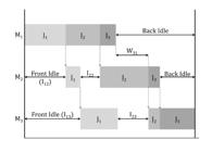
The idle time ($I_{jk}$) on machine $k$ before the operation job $j$ is initiated is defined by the time between the beginning of job j operation and the completion of the previous job. If job $j$ is the first in the schedule, the idle time on machines $k\in M\setminus \left\{1\right\}$ is defined as front idle as the schedule starts at time 0 and is obtained by the difference between time 0 and its beginning time in each machine. It is considered that the operation of the first job is initiated at time 0. The interval between the completion time of the last job in each machine $k\in M\setminus \left\{m\right\}$ and the makespan is defined as back idle ($B{I}_k$). The waiting time ($W_{jk}$) of job $j$ in machine $k$ is the time between its completion in the machine and its beginning in the next machine.

Figure 1 presents a Gantt chart for a $3\times 3$ scheduling problem (3 jobs and 3 machines) and highlights its machines idle times, job waiting times, front idle times, and back idle times. Maassen et al. (2020) classified scheduling problems that consider idle time in three different ways: (1) including back and front idle times; (2) excluding both back and front idle times; and (3) including front idle time but not back idle time. In this paper, we consider the third definition as part of our objective function because it is assumed that the final gap (back idle time) could be used to start another schedule of jobs.

Figure 1
Illustrative example of a 3x3 scheduling problem.

It is important to notice that if the first definition is considered, the minimisation of the total idle time (front, core and back) may be equivalent to minimising makespan, as observed by Framinan et al. (2003) and Fernandez-Viagas & Framinan (2014).

A mathematical representation of the addressed problem is presented as a position-based mixed-integer linear programming (MILP) model that was introduced by Abreu & Fuchigami (2022). This model proved to be robust and efficient in handling the minimisation of total sum of core and front idle time and core waiting time as solved small size instances (up to 12 jobs and machines) optimally.

Let the binary variable $x_{jh}=1$ if the job $j\in N$ is scheduled in the position $h\in S$ of the sequence, and 0 otherwise. Variable $C_{hk}$ indicates the completion time of the job in $h$ position in machine $k$. The idle time on machine $k$ before the job in position $h$ is given by $I_{hk}$. Finally, $W_{hk}$ represents the waiting time of job in position $h$ on machine $k$. For an extensive experimentation of this and other mathematical formulations the reader is referred to Abreu & Fuchigami (2022).

$\min {\displaystyle \sum }_{h\in S}{\displaystyle \sum }_{k\in M}\left(I_{hk}+W_{hk}\right),$ (1)

Subject to

${\displaystyle \sum }_{h\in S}{x}_{jh}=\mathrm{1,}j\in N,$ (2)

${\displaystyle \sum }_{j\in N}{x}_{jh}=\mathrm{1,}h\in S,$ (3)

$C_{11}={\displaystyle \sum }_{j\in N}{p}_{j1}{x}_{j1},$ (4)

$C_{h,k+1}-C_{hk}-W_{hk}={\displaystyle \sum }_{j\in N}{p}_{j,k+1}{x}_{jh},h\in S,k\in M\setminus \left\{m\right\},$ (5)

$C_{h+\mathrm{1,}k}-C_{hk}-I_{h+\mathrm{1,}k}={\displaystyle \sum }_{j\in N}{p}_{jk}{x}_{j,h+1},h\in S\setminus \left\{n\right\},k\in M,$ (6)

$I_{\mathrm{1,}k+1}=I_{1k}+W_{1k}+{\displaystyle \sum }_{j\in N}{p}_{jk}{x}_{j1},k\in M\setminus \left\{m\right\},$ (7)

$x_{jh}\in \left\{\mathrm{0,1}\right\},j\in N,h\in S,$ (8)

$C_{hk},I_{hk},W_{hk}\ge \mathrm{0,}h\in S,k\in M.$ (9)

Equation 1 represents the objective of minimising the machine’s idle time and the job waiting time. Notice that this is a sum-form objective function. Constraints 2 and 3 ensure that only one job is assigned to each position and that each position is occupied by just one job. Constraint 4 defines the completion time of the first job on the first machine as its processing time ensuring that the operations initiate at time 0. Constraints 5 express the difference between the completion time of a job $j$ on two consecutive machines ($k$ and $k+1$) as its waiting time on machine $k$ plus its processing time on machine $k+1$. Constraints 6 indicate that the difference between the completion times of two consecutive jobs on a machine is equal to the processing time of the second (of both jobs) plus its idle time. Constraints 7 define the front idle on each machine. The variables domain is defined in 8 and 9.

4. Methodology

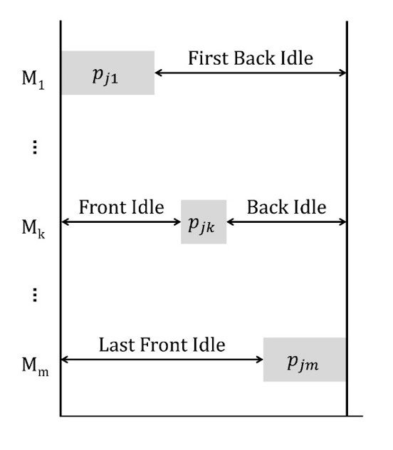
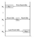
The use of operational metrics to sort jobs is simple to be implemented and is highly used in practice. However, as more complex manufacturing systems become, the need of more specific measures increases. We introduce four tailored metrics based on the machine idle times caused by each job as shown in Figure 2 . These measures were designed for the permutation flow shop scheduling problem when the least unproductive time is desired.

Figure 2
Representation of the scheduling metrics.

4.1. Tailored scheduling metrics

As basis of comparison, we also use two dispatching rules that are common in the scheduling literature. Both rules are based on the total processing time, i.e., each job $j$ is assigned a total processing time in which consists in summing the processing time of this job on all machines. The dispatching rule Longest Processing Time (LPT) sorts jobs in decreasing order of total processing time while the rule Shortest Processing time (SPT) sorts them in an ascending order. Additionally, we generate random sequences. As follows we first introduce the metrics that are computed for each job and then we detail the algorithmic procedure of insertion to optimise the initial solution.

The front idle time is incorporated in two ways. The first approach is to sum the front idle time on each machine, resulting in two scheduling rules. The Longest Front Idle Time rule (LFIT) sorts the jobs in the order of decreasing total front idle times. Its counterpart is the Shortest Front Idle Time rule (SFIT) which sorts the jobs in the order of ascending total front idle times ($F{I}_j$).

$F{I}_j={{\displaystyle \sum }}_{k\in M}\left(m-k\right)p_{jk},j\in N.$ (10)

The second approach consists in sorting jobs based on the idle time on the last machine. In this approach, we also have two scheduling rules. The Longest Last Front Idle Time rule (LLFIT) which sorts in the order of decreasing last front idle times ($LF{I}_j$) as calculated by the Equation 11. Its counterpart is the Shortest Last Front Idle Time rule (SLFIT) which sorts jobs in the order of ascending the last front idle times ($LF{I}_j$).

$LF{I}_j={{\displaystyle \sum }}_{k\in M\setminus \left\{m\right\}}{p}_{jk},j\in N.$ (11)

The back idle time is also incorporated in two ways. The first approach considers the total back idle time and results in two scheduling rules. The Longest Back Idle Time rule (LBIT) sorts the jobs in the order of decreasing total back idle times ($B{I}_j$) as calculated by the Equation 12. Its counterpart is the Shortest Back Idle Time rule (SBIT) in which sorts the jobs in the order of ascending total back idle time ($B{I}_j$).

$B{I}_j={{\displaystyle \sum }}_{k\in M\setminus \left\{1\right\}}\left(k-1\right)p_{jk},j\in N.$ (12)

The second approach based on back idle time consists in sorting jobs considering only the first back idle time, i.e., the machine idle time after the job’s completion time on the first machine and its completion time on the last machine. This metric results in two scheduling rules. The Longest First Back Idle Time rule (LFBIT) sorts the jobs in the order of decreasing first back idle times ($FB{I}_j$) as calculated by the Equation 13. Its counterpart is the Shortest First Back Idle Time rule (SFBIT), and it sorts the jobs in the order of ascending first back idle times ($FB{I}_j$).

$FB{I}_j={{\displaystyle \sum }}_{k\in M\setminus \left\{1\right\}}{p}_{jk},j\in N.$ (13)

In summary, we incorporate eight scheduling rules designed to generate efficient solutions considering the minimisation of idle and waiting times.

4.2. Heuristic insertion procedure

An improvement heuristic procedure was formulated based on rules defined previously and the insertion method of the Nawaz et al. (1983) algorithm. We choose the NEH heuristic procedure to implement and compare new idle-time-based rules based on: (i) the results of Framinan et al. (2003) and Maassen et al. (2019); (ii) its versatility for different problems; (iii) good performance on many scheduling variants; and (iv) the simplicity of understanding and implementation.

From an initial scheduling solution, this heuristic procedure attempts to optimise the objective function by iteratively inserting a job into a partial solution while maintaining the relative position among jobs already sorted. The initial sequence $\pi \text{'}$ is obtained by applying one of the tailored scheduling metrics presented in Section 4.1. only once. Thus, resulting in different a solution depending on the rule used. The pseudocode of the $NE{H}_{IW}$ heuristic is described in Algorithm 1 as follows.

Algorithm 1:$NE{H}_{IW}$ heuristic procedure

1: Input: Processing time $p_{jk}$, initial sequence ${\pi }^{\prime }$.

2: Output: Optimised sequence $\pi$.

3: ${\pi }^{\prime }=\left\{{\pi }_1^{\text{'}},\dots ,{\pi }_n^{\text{'}}\right\}$

4: procedure$NE{H}_{IW}\left(p_{jk},\pi \text{'}\right)$

5: $\pi =\varnothing$ $⊳$ Initialise the optimised sequence

6: $\pi \leftarrow \left\{{\pi }_1^{\text{'}}\right\}$

7: $n_s=1$ $⊳$ Number of sorted jobs

8: for$h=\mathrm{2,}\dots ,n$do

9: Test ${\pi }_h^{\text{'}}$ in each position keeping the relative position

10: for$l=\mathrm{1,}\dots ,n_s+1$do

11: ${\pi }_l^{\text{'}\text{'}}={\pi }_h^{\text{'}}$ $⊳$ Initialise test sequence

12: $\left({\pi }_1^{\text{'}\text{'}},\dots ,{\pi }_{l-1}^{\text{'}\text{'}}\right)=\left({\pi }_1^{\text{'}},\dots ,{\pi }_{l-1}^{\text{'}}\right)$ $⊳$ Duplicate first $l-1$ positions

13: $\left({\pi }_{l+1}^{\text{'}\text{'}},\dots ,{\pi }_{n_s+1}^{\text{'}\text{'}}\right)=\left({\pi }_l^{\text{'}},\dots ,{\pi }_{n_s}^{\text{'}}\right)$ $⊳$ Duplicate the rest of positions

14: Check the objective function $IW\left({\pi }^{″}\right)$

15: end for

16: ${\pi }^{\prime }\leftarrow {\pi }^{″}$ with the least $IW\left({\pi }^{″}\right)$

17: $n_s++$ $⊳$ Update the number of sorted jobs

18: end for

19: $\pi \leftarrow {\pi }^{\prime }$

20: end procedure

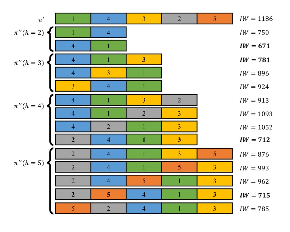
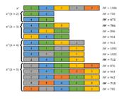
As an example, consider an instance with 5 jobs and 5 machines, where the processing times of the jobs on each machine are $p_1=\left(\mathrm{58,}\mathrm{77,}\mathrm{53,}\mathrm{99,}39\right)$, $p_2=\left(\mathrm{1,}\mathrm{58,}\mathrm{13,}\mathrm{71,}64\right)$, $p_3=\left(\mathrm{93,}\mathrm{4,}\mathrm{62,}\mathrm{22,}31\right)$, $p_4=\left(\mathrm{39,}\mathrm{81,}\mathrm{67,}\mathrm{51,}69\right)$, $p_5=\left(\mathrm{18,}\mathrm{15,}\mathrm{24,}\mathrm{69,}25\right)$, where $p_i$ contains the processing times of job $i$. The initial sequence is obtained by sorting the jobs using the LLFIT rule, resulting in the solution ${\pi }^{\prime }=\left(\mathrm{1,4,3,2,5}\right)$ with an objective function of 1186. Then we run the $NE{H}_{IW}$ algorithm. At first, we check the best permutation of the first two jobs. We keep their relative position and test inserting the next job of the initial solution. These steps are executed until the last job is inserted. Each iteration of the $NE{H}_{IW}$ algorithm is illustrated in Figure 3.

Figure 3
Illustrative example of how NEH works.

Additionally, we have implemented the heuristic from Fernandez-Viagas & Framinan (2015) for comparison. The proposed algorithm, hereafter referred to as FF, is a constructive heuristic that starts by ranking jobs using an indicator that combines the induced idle and completion times. Based on this ranking, an initial partial sequence is built, and jobs are iteratively included considering the indicator value.

5. Design of experiments

5.1. Experimental setup

All procedures were tested in 72 sets with 10 instances of processing times. Each set of instances uses a different combination of problem size $n\times m$ ($n$ jobs and $m$ machines). In total, we implemented all algorithms in each one of the 720 benchmark instances. The algorithms were written and implemented in the Julia syntax using the environment JuliaPro 1.5. All experiments were performed on an Intel Core i7-8565U 1.80 GHz machine (in 64 bits mode) with 8 GB memory and Windows Operations System and the results are publicly available on https://github.com/abreualexp/fs_neh_iw. The benchmarks are described as follows.

• 120 of these instances were generated with the parameters for flow shop problem proposed by Taillard (1993) considering the sizes of $n\in \left\{\mathrm{3,}\mathrm{4,}\mathrm{5,}\mathrm{8,}\mathrm{10,}\mathrm{12,}\mathrm{15,}20\right\}$ and $m\in \left\{\mathrm{3,}\mathrm{5,}\mathrm{6,}\mathrm{8,}\mathrm{10,}\mathrm{12,}15\right\}$ used by Ku & Beck (2016).

• 120 of the instances consist of the original benchmark sets of Taillard (1993) considering the sizes of $n\in \left\{\mathrm{20,}\mathrm{50,}\mathrm{100,}\mathrm{200,}500\right\}$ and $m\in \left\{\mathrm{5,}\mathrm{10,}20\right\}$.

• 240 of the instances are the original VRF benchmark sets of Vallada et al. (2015), considering small sizes of $n\in \left\{\mathrm{10,}\mathrm{20,}\mathrm{30,}\mathrm{40,}\mathrm{50,}60\right\}$ and $m\in \left\{\mathrm{5,}\mathrm{10,}\mathrm{15,}20\right\}$.

• 240 of the instances are the original VRF benchmark sets of Vallada et al. (2015), considering large sizes of $n\in \left\{\mathrm{100,}\mathrm{200,}\mathrm{300,}\mathrm{400,}\mathrm{500,}\mathrm{600,}\mathrm{700,}800\right\}$ and $m\in \left\{\mathrm{20,}\mathrm{40,}60\right\}$.

In order to evaluate both solution results and computational times we applied the Relative Deviation Index (RDI) which is obtained for each method and instance and is bounded by [0, 100]. This evaluation criterion was also applied by Vallada et al. (2008) to analyse the results of heuristics and metaheuristics for a flow shop problem.

$RD{I}_{Method}=100\frac{I{W}_{Method}-I{W}_{Best}}{I{W}_{Worst}-I{W}_{Best}}.$ (14)

In this criterion, Best and Worst are the best and the worst results obtained among all the methods, respectively. With this measure, a value between 0 and 100 is obtained for each method such that a good solution will be close to 0. If the worst and the best results are the same, i.e. all the methods provided the same solution, its RDI value will be 0.

5.2. Computational results

5.2.1. Rules’ results

Initially, the solutions of each scheduling rule were analysed among other scheduling rules, i.e., only the 11 priority rules presented in Section 4.1. were used to compute the RDI. Table 2 shows for each rule its percentage of success (amount of times that achieved $RDI=0$ in relation to all 720 instances), percentage of failures (amount of times that achieved $RDI=100$ also in relation to all 720 instances), and average RDI (ARDI). The top three best algorithms for each statistic are highlighted in bold.

Table 2
Main statistics of the scheduling rules.

Rules	Success (%)	Failures (%)	Solution ARDI (%)
LFBIT	1.94	10.83	54.98
LBIT	3.75	4.03	45.02
LLFIT	1.25	6.81	45.54
LFIT	17.08	6.94	34.29
LPT	1.53	5.69	43.98
RAND	4.86	2.64	32.23
SFBIT	38.89	1.25	11.91
SBIT	1.94	3.61	41.41
SLFIT	19.03	0.42	13.67
SFIT	6.11	65.83	81.42
SPT	16.39	0.69	14.74

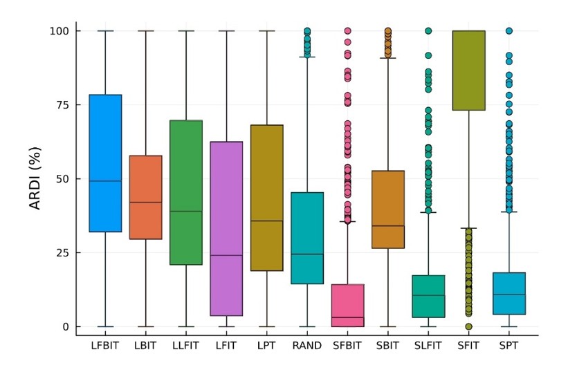
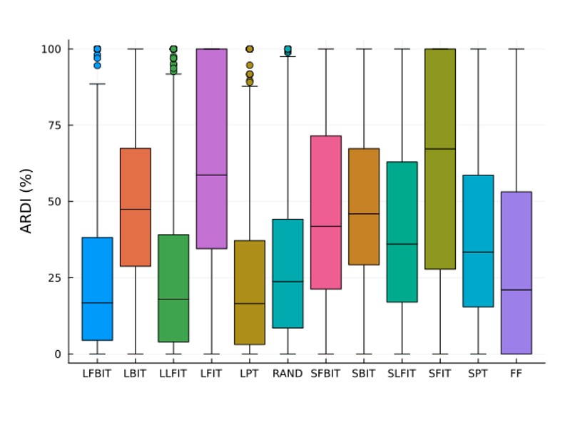
Figure 4 presents the boxplot chart of each scheduling rule. This chart highlights the central, upper, and lower quartiles (rectangle), the median (horizontal line), minimum, maximum, and outliers.

Figure 4
Boxplot of each scheduling rule performance.

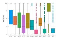
From Table 2 and Figure 4, it is observed that the rules with better performance are SFBIT, SLFIT, and SPT, respectively. We highlight that the ascending order presented better results even with the SFIT outlier. The rules that considered all front or back idle did not present good solutions at all. Rules with descending order performed more uniformly.

Table 3 shows how worst is each scheduling rule solution in comparison to the optimal solutions found in Abreu & Fuchigami (2022). This analysis was carried out using 100 instances of up to 12 job and 12 machines. For each method and instance, we compute $100\left(\frac{rule\_solution}{optimal\_solution}-1\right)$. In general, the solutions found using the rules with the decreasing order of metrics were outperformed by the rules that use the increasing order of each metric. Additionally, only rules SLFIT, SFIT, and SPT were able to find the optimal solution for more than 10% of the instances analysed (13%, 15%, and 11%, respectively).

Table 3
Difference between the scheduling rules’ solution and the optimal solution.

$n\times m$	LFBIT	LBIT	LLFIT	LFIT	LPT	RAND	SFBIT	SBIT	SLFIT	SFIT	SPT
3x3	79.81	31.32	99.05	105.99	93.25	61.54	35.22	77.08	16.56	15.95	20.92
3x6	28.91	25.66	34.05	37.65	31.56	23.64	12.63	23.60	6.36	3.64	7.98
3x8	18.50	16.01	25.25	30.23	23.74	9.48	15.28	14.37	5.17	4.98	12.55
3x10	15.65	8.31	15.51	21.00	14.99	15.04	11.69	16.17	10.24	5.83	10.97
4x3	86.56	49.43	106.24	110.00	89.02	60.23	53.03	78.87	21.60	52.72	31.18
5x3	197.51	133.68	187.83	174.65	189.07	145.05	90.58	144.99	58.54	90.03	68.46
5x5	75.76	55.49	80.72	90.39	85.62	59.56	52.44	67.55	25.49	31.16	18.28
8x8	59.05	62.32	70.17	71.20	71.25	40.90	43.40	48.00	33.34	41.97	33.99
10x10	56.91	50.61	65.31	59.18	65.79	56.87	40.13	52.93	39.70	44.24	36.42
12x12	62.08	42.73	61.59	63.73	60.66	56.19	44.81	52.39	41.83	41.22	43.44
Avg.	68.07	47.56	74.57	76.40	72.50	52.85	39.92	57.59	25.88	33.17	28.42

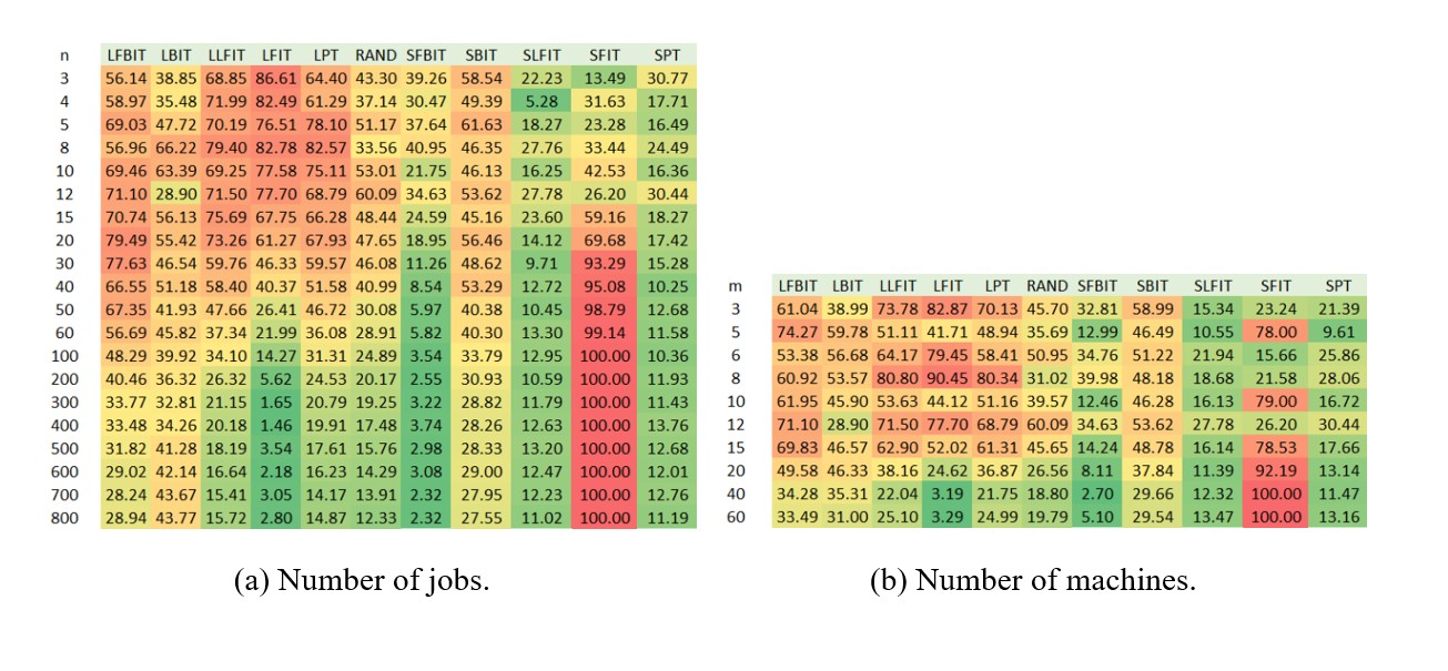
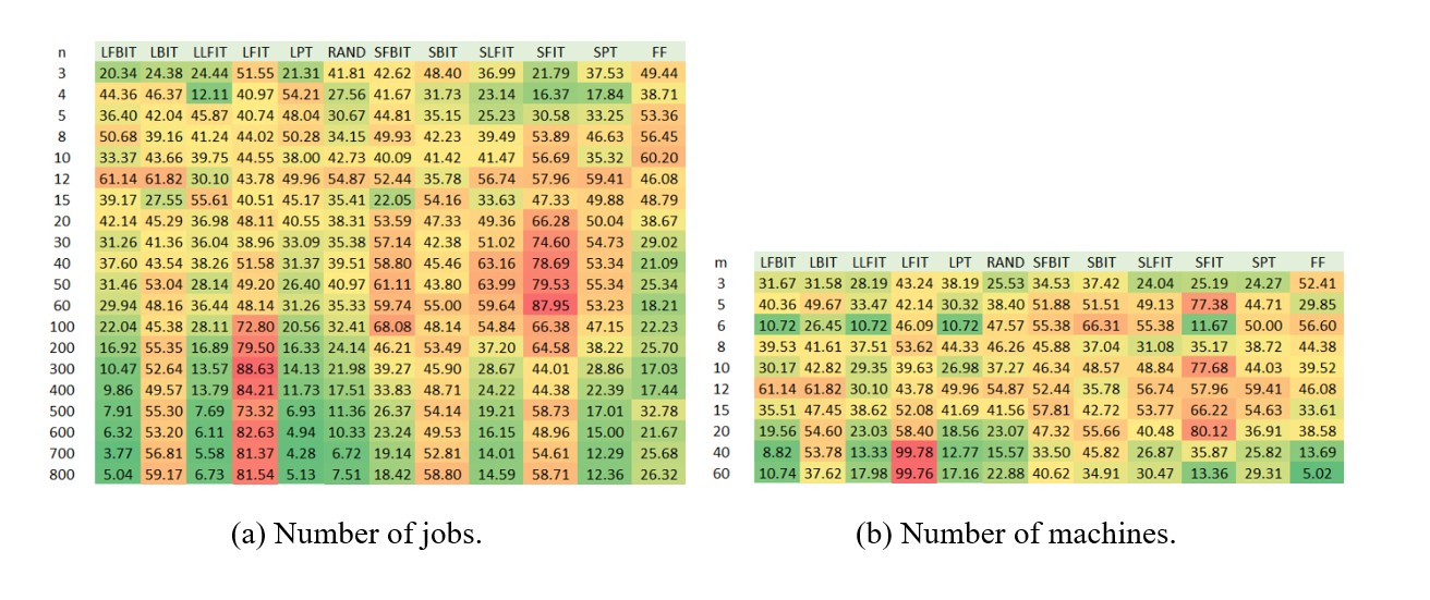
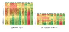
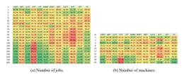
Figure 5 provides the scheduling rules’ average RDI for different sizes of jobs ($n$) and machines ($m$). We observe that, for a small number of either $n$ or $m$, the rules that use the decreasing order of each metric find worst solutions. It is also seen that, except for the rule SFIT, the rules that use the increasing order of metrics have better performance as the instance’s size increases.

Figure 5
Average RDI of the scheduling rules for different sizes of instance.

5.2.2. Heuristics’ results

It is expected that any rule performance would be improved with the heuristic insertion procedure. To evaluate these algorithms, the solutions obtained by the heuristics were also analysed separately, i.e., only the 12 heuristic methods presented in Section 4.2 were used to compute the RDI. Table 4 summarise each heuristic percentage of success, percentage of failures, solution ARDI, and computational time ARDI. The top three best algorithms for each statistic are also highlighted in bold.

Table 4
Main statistics of the heuristics.

Heuristics	Success (%)	Failures (%)	Solution ARDI (%)	Time ARDI (%)
LFBIT	16.94	3.06	25.33	33.34
LBIT	8.75	5.69	47.57	39.22
LLFIT	18.47	3.19	26.17	33.26
LFIT	6.25	29.03	60.37	41.73
LPT	18.89	5.00	25.23	49.34
RAND	10.83	3.75	30.29	38.01
SFBIT	7.78	10.14	46.29	33.73
SBIT	7.08	6.67	47.66	40.43
SLFIT	7.64	5.83	41.41	33.60
SFIT	7.36	28.06	60.66	31.75
SPT	7.64	5.28	39.09	30.03
FF	29.72	9.58	31.57	0.13

From Table 4 and Figure 6, the heuristics that consider as initial solution the rules that assign jobs in a descending order of the metrics achieved better results. Regarding the solution quality statistics (success, failures, and RDI), LLFIT can be assumed as the best heuristic over all others for being in top three best algorithms, followed by LFBIT and LPT which are in top three in two statistics. As observed before, the heuristics which consider all front or back idle did not present good results. However, regarding the computational time, the FF heuristic outperforms all other algorithms while also presents the highest percentage of best solutions (column “Success”).

Figure 6
Boxplot of each heuristic’s performance.

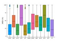
Table 5 shows how worst is each heuristic’s solution in comparison to the optimal solutions found in Abreu & Fuchigami (2022). This analysis was carried out using the same instances as in Table 3. In general, see that the heuristics that use decreasing order of metrics as initial solution provide better solutions. In fact, apart from SFIT as initial solution, the only heuristics that found more than 20% of optimal solutions used LFBIT, LBIT, LLFIT, and LPT (23%, 21%, 21%, and 20%, respectively).

Table 5
Difference between the heuristics’ solution and the optimal solution.

$n\times m$	LFBIT	LBIT	LLFIT	LFIT	LPT	RAND	SFBIT	SBIT	SLFIT	SFIT	SPT	FF
3x3	6.07	6.07	13.14	23.60	6.86	6.92	11.83	12.95	7.59	7.64	10.97	23.35
3x6	4.18	6.42	4.18	8.27	4.18	8.06	7.74	8.97	7.74	3.16	6.70	7.98
3x8	3.07	4.96	3.76	9.50	4.23	7.80	7.66	3.26	3.12	2.40	6.14	5.24
3x10	1.64	1.28	1.82	4.77	1.69	2.38	5.09	5.10	6.38	3.99	4.91	8.79
4x3	20.12	21.09	10.99	28.67	26.35	16.69	25.91	22.46	13.67	8.84	17.99	22.82
5x3	33.91	25.63	40.03	34.26	36.44	30.11	27.64	36.66	26.08	26.37	28.99	48.79
5x5	15.16	17.93	16.59	15.20	21.29	10.09	13.87	7.62	8.69	11.99	9.30	11.90
8x8	17.96	17.35	16.61	16.85	17.82	15.03	17.94	16.72	15.25	19.61	16.60	20.33
10x10	16.51	19.72	25.70	18.64	19.94	17.04	15.81	24.09	22.89	25.15	17.33	25.57
12x12	23.62	23.96	16.99	20.60	21.56	21.93	22.44	18.14	22.75	23.22	24.04	20.03
Avg.	14.22	14.44	14.98	18.03	16.03	13.61	15.59	15.60	13.41	13.24	14.30	19.48

Figure 7 provides the scheduling rules’ average RDI for different sizes of jobs and machines. These results are more uniformly distributed, in comparison to Figure 5. However, notice that the heuristics that use the decreasing order of metrics as initial solution provide now better results, even as the size of either jobs or machines increases.

Figure 7
Average RDI of the heuristic algorithms for different sizes of instance.

5.2.3. Comparative analysis

In this section, we provide a comparative analysis of the NEH insertion procedure. Tables 6 to 8 provide comparisons of ARDI, percentage of success, and percentage of failures between rules and heuristics, respectively. Since each scheduling rule presented in Section 4.1. is used as initial solution for the NEH, we evaluate the impact of this insertion procedure. From the definition of the procedure, we know that the final heuristic’s solution is at least equal to the provided initially. Note that the values in the rules’ column are computed only among the rules, and the values in the heuristics’ column are computed only among heuristics. For instance, in Table 7, the LFBIT scheduling rule has better solutions for 1.94% of instances (compared with other rules only), while using LFBIT as initial solution for the insertion procedure results in better solutions for 25.69% of instances (compared with other heuristics only).

Table 6
Rules and heuristics ARDI comparison.

Procedures	Rules ARDI (%)	Heuristics ARDI (%)	Difference (%)
LFBIT	54.98	22.58	-58.93
LBIT	45.02	46.00	2.18
LLFIT	45.54	23.76	-47.83
LFIT	34.29	59.64	73.93
LPT	43.98	22.59	-48.64
RAND	32.23	27.92	-13.37
SFBIT	11.91	45.23	279.81
SBIT	41.41	45.90	10.84
SLFIT	13.67	40.09	193.33
SFIT	81.42	60.10	-26.19
SPT	14.74	37.56	154.83

Table 8
Rules and heuristics percentage of failures comparison.

Procedures	Rules failure (%)	Heuristics failure (%)	Difference (%)
LFBIT	10.83	3.75	-65.38
LBIT	4.03	6.39	58.62
LLFIT	6.81	4.03	-40.82
LFIT	6.94	30.42	338.00
LPT	5.69	5.69	0.00
RAND	2.64	4.31	63.16
SFBIT	1.25	10.97	777.78
SBIT	3.61	7.64	111.54
SLFIT	0.42	6.81	1533.33
SFIT	65.83	30.83	-53.16
SPT	0.69	6.39	820.00

Table 7
Rules and heuristics percentage of success comparison.

Procedures	Rules success (%)	Heuristics success (%)	Difference (%)
LFBIT	1.94	25.69	1221.43
LBIT	3.75	10.00	166.67
LLFIT	1.25	23.33	1766.67
LFIT	17.08	7.22	-57.72
LPT	1.53	23.33	1427.27
RAND	4.86	14.17	191.43
SFBIT	38.89	7.92	-79.64
SBIT	1.94	8.06	314.29
SLFIT	19.03	8.47	-55.47
SFIT	6.11	9.72	59.09
SPT	16.39	8.61	-47.46

The top three best results are highlighted in bold. The comparison of performances is carried out through the $difference=\left(\frac{heuristic}{rule}-1\right)100$. Therefore, the best values of difference are the lowest for ARDI and percentage failures comparisons, and the highest for percentage success.

In terms of ARDI, we can observe an explicit inversion of performance from Table 6. The top three rules were SFBIT, SLFIT, and SPT, however, they had its performance worsened with the heuristic’s insertion procedure (variation of 279.81%, 193.33%, and 154.83%, respectively). Yet, the heuristics LFBIT, LPT, and LLFIT are the ones that improved the most with the procedure and achieved the top three best results of ARDI (variation of −58.93%, −48.64%, and −47.83%, respectively), especially the LFBIT and LLFIT which went from one of the worst rules to the best heuristics.

For the percentage of success (amount of times that achieved $RDI=0$ in relation to all 720 instances), Table 7 shows almost the same result as previous tables. The heuristics LFBIT, LPT, and LLFIT are the ones that improved the most with the heuristic insertion procedure (variation of 1221.43%, 1427.27%, and 1766.67%) and achieved the top three best results (success of 25.69%, 23.33%, and 23.33%, respectively). But for the rules, SFBIT, SLFIT, and LFIT, which were the top three rules, had their outputs worsened with the procedure, especially SFBIT and LFIT which are the ones that got worst (variation of −79.64% and −57.72%, respectively) and performed poorly with the procedure (success of 7.92% and 7.22%, respectively).

Regarding the percentage of failures (amount of times that achieved $RDI=100$, also in relation to all 720 instances), the best performing rules were SLFIT, SPT, and SFBIT. However, these rules had the worst variation when provided as initial solution for the heuristic procedure especially the SFBIT rule which went from one of the best to one of the worst performances. Although the rule SFIT had one of the biggest improvements (−53.16%), it remained among the worst results. The LFBIT procedure went from the second worst rule to the best heuristic achieving the variation of −65.38%. It is observed that the LPT procedure achieved the same performance in both the rule and heuristic algorithms.

In general, it is worth noticing, from Tables 6 to 8, that some scheduling rules that perform poorly on their own can still produce initial solutions that the insertion heuristic improves by a large margin.

5.3. Performance profile analysis

Additionally, we provide a visual representation of each method’s relative performance through performance profiles as proposed by Dolan & Moré (2002). This evaluation methodology presents a clear indication of the relative performance of each method as means of providing objective information when comparing optimisation algorithms (Gould & Scott, 2016). Some recent and interesting works on various scheduling problems that successfully took advantage of this methodology on its evaluation process are Moreno et al. (2019), Abreu & Fuchigami (2022), Freitas & Fuchigami (2022), and Fuchigami & Abreu (2024).

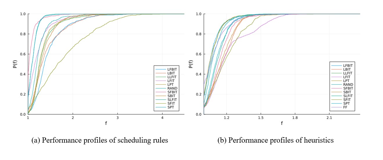
The performance profile provides the method’s cumulative distribution function that indicates the experimental probability of its performance ratio ($P\left(f\right)$) is within an interest factor ($f$) among all solved instances. The performance profile of an algorithm computes its relative performance for each instance, e.g., the ratio of its solution by the solution of the best performing method. Then, it is shown the proportion of instances in which the algorithm presented a relative performance up to a factor of interest. Figure 8 presents the performance profiles of all scheduling rules and heuristics.

Figure 8
Performance profiles of the methods.

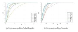
Figure 8a presents the performance profile of each scheduling rule among all 720 instances. We can observe that the ascending way of ordering has outperformed the descending way, with the exceptions of the LFIT (that presented more success than all other rules) and the SFIT (that presented the largest amount of failures). It is also possible to observe three groups of rules with similar behaviour. The first one contains just the SFIT rule and has clearly the worst performance. The second group consists of the LFIT, SFBIT, SLFIT, and SPT. The remainder rules, which form the third group, have average performance and similar curve behaviours. We highlight that the consideration of all front or back idle presented some of the worst results.

Figure 8b shows the performance profile of each heuristic among all 720 instances. With the insertion procedure, the heuristics curve behaviour has moved to a more similar output. It is still possible to note that there are three heuristics that outperform the other in terms of curve behaviour.

6. Concluding remarks

We study a manufacturing system in which jobs are scheduled to be processed in the same sequence on a set of machines. The defined sequence must be one with the least unproductive time that consists in the time machines are not processing any job and a job is not processed on any machine. Based on the operational research literature, this system can be represented as a permutational flow shop scheduling problem with machine idle time and job waiting time minimisation.

Our literature review showed that no study has extensively compared metrics along with heuristics algorithms for this problem. We developed four tailored metrics designed to find high quality solutions for this scheduling problem and compared them with classic rules. Additionally, an insertion heuristic algorithm is implemented to further improve the metrics’ solutions.

The impact of the algorithm on each metric is comprehensively evaluated. Our computational experimentation consists in 720 instances from four benchmarks with different combinations of number of jobs and number of machines. We analyse each method’s results with based on percentage of success and failure, average relative deviation index, and computational time.

Among the insertion heuristic algorithms, the LFBIT, LLFIT, and LPT obtained the best results in all analysed statistics. In general, the heuristic which considers the Longest Last Front Idle Time rule (LLFIT) as initial solution outperformed the remainder algorithms. Although this method is not the top one in all statistics, it was the only procedure that was in the top three for all statistics. Therefore, we conclude that the LLFIT heuristic had the best performance for the total sum of core and front idle time and core waiting time minimisation.

Unlike what was found by Framinan et al. (2003) for core idle time and by Maassen et al. (2019) for core waiting time, the original configuration of the NEH heuristic was not able to outperform our idle-time-based scheduling rules as the initial solution for the insertion procedure. In short, the LLFIT rule is more efficient for the problem addressed than the LPT. Therefore, since job scheduling plays an important role in production and operations management, our results contribute to practitioners which face similar problems and prefer fast and good-enough solutions.

Since our research were designed to evaluate the performance of the new metrics in the problem addressed, it is not possible to extend our conclusions for a broad amount of other scheduling variant problems. Then, testing our algorithms in different manufacturing systems, such as non-permutational scheduling, incorporation of blocking, and allowance of preemption or interruption, poses as further research opportunities. Furthermore, as new production measures with a minimum negative impact on the environment continuously increases, efficient methods to improve energy consumption, reduce waste, and unproductive times.

• How to cite this article: Abreu, A., & Fuchigami, H. Y. (2026). Optimising manufacturing schedules with tailored metrics to reduce unproductive times. Production, 36, e20250004. https://doi.org/10.1590/0103-6513.20250004
• Financial Support
  This research was funded by the São Paulo Research Foundation (FAPESP, grant number 2022/05803-3) and the Brazilian National Council for Scientific and Technological Development (CNPq, grant numbers 154540/2019-6 and 135179/2020-3)
• Ethical Statement
  This research did not require ethical approval
• Data availability
  Research data is available in a repository.

References

• Abreu, A. P., & Fuchigami, H. Y. (2022). An efficiency and robustness analysis of warm-start mathematical models for idle and waiting times optimization in the flow shop. Computers & Industrial Engineering, 166, 107976. https://doi.org/10.1016/j.cie.2022.107976
  » https://doi.org/10.1016/j.cie.2022.107976
• Alfieri, A., Garraffa, M., Pastore, E., & Salassa, F. (2023). Permutation flowshop problems minimizing core waiting time and core idle time. Computers & Industrial Engineering, 176, 108983. https://doi.org/10.1016/j.cie.2023.108983
  » https://doi.org/10.1016/j.cie.2023.108983
• Alidaee, B., Li, H., Wang, H., & Womer, K. (2021). Integer programming formulations in sequencing with total earliness and tardiness penalties, arbitrary due dates, and no idle time: A concise review and extension. Omega, 103, 102446. https://doi.org/10.1016/j.omega.2021.102446
  » https://doi.org/10.1016/j.omega.2021.102446
• Allahverdi, A. (2016). A survey of scheduling problems with no-wait in process. European Journal of Operational Research, 255(3), 665-686. https://doi.org/10.1016/j.ejor.2016.05.036
  » https://doi.org/10.1016/j.ejor.2016.05.036
• Allahverdi, A., Aydilek, H., & Aydilek, A. (2020). No-wait flowshop scheduling problem with separate setup times to minimize total tardiness subject to makespan. Applied Mathematics and Computation, 365, 124688. https://doi.org/10.1016/j.amc.2019.124688
  » https://doi.org/10.1016/j.amc.2019.124688
• An, Y. J., Kim, Y. D., & Choi, S. W. (2016). Minimizing makespan in a two-machine flowshop with a limited waiting time constraint and sequence-dependent setup times. Computers & Operations Research, 71, 127-136. https://doi.org/10.1016/j.cor.2016.01.017
  » https://doi.org/10.1016/j.cor.2016.01.017
• Arviv, K., Stern, H., & Edan, Y. (2016). Collaborative reinforcement learning for a two-robot job transfer flow-shop scheduling problem. International Journal of Production Research, 54(4), 1196-1209. https://doi.org/10.1080/00207543.2015.1057297
  » https://doi.org/10.1080/00207543.2015.1057297
• Balogh, A., Garraffa, M., O’Sullivan, B., & Salassa, F. (2022). MILP-based local search procedures for minimizing total tardiness in the No-idle Permutation Flowshop Problem. Computers & Operations Research, 146, 105862. https://doi.org/10.1016/j.cor.2022.105862
  » https://doi.org/10.1016/j.cor.2022.105862
• Baraz, D., & Mosheiov, G. (2008). A note on a greedy heuristic for flow-shop makespan minimization with no machine idle-time. European Journal of Operational Research, 184(2), 810-813. https://doi.org/10.1016/j.ejor.2006.11.025
  » https://doi.org/10.1016/j.ejor.2006.11.025
• Bektaş, T., Hamzadayı, A., & Ruiz, R. (2020). Benders decomposition for the mixed no-idle permutation flowshop scheduling problem. Journal of Scheduling, 23(4), 513-523. https://doi.org/10.1007/s10951-020-00637-8
  » https://doi.org/10.1007/s10951-020-00637-8
• Birgin, E. G., Ferreira, J. E., & Ronconi, D. P. (2020). A filtered beam search method for the m-machine permutation flowshop scheduling problem minimizing the earliness and tardiness penalties and the waiting time of the jobs. Computers & Operations Research, 114, 104824. https://doi.org/10.1016/j.cor.2019.104824
  » https://doi.org/10.1016/j.cor.2019.104824
• Cheng, C. Y., Ying, K. C., Li, S. F., & Hsieh, Y. C. (2019). Minimizing makespan in mixed no-wait flowshops with sequence-dependent setup times. Computers & Industrial Engineering, 130, 338-347. https://doi.org/10.1016/j.cie.2019.02.041
  » https://doi.org/10.1016/j.cie.2019.02.041
• Freitas, M. G., & Fuchigami, H. Y. (2022). A new technology implementation via mathematical modeling for the sequence-dependent setup times of industrial problems. Computers & Industrial Engineering, 172, 108624. https://doi.org/10.1016/j.cie.2022.108624
  » https://doi.org/10.1016/j.cie.2022.108624
• Dolan, E. D., & Moré, J. J. (2002). Benchmarking optimization software with performance profiles. Mathematical Programming, 91(2), 201-213. https://doi.org/10.1007/s101070100263
  » https://doi.org/10.1007/s101070100263
• Fernandez-Viagas, V., & Framinan, J. M. (2014). On insertion tie-breaking rules in heuristics for the permutation flowshop scheduling problem. Computers & Operations Research, 45, 60-67. https://doi.org/10.1016/j.cor.2013.12.012
  » https://doi.org/10.1016/j.cor.2013.12.012
• Fernandez-Viagas, V., & Framinan, J. M. (2015). A new set of high-performing heuristics to minimise flowtime in permutation flowshops. Computers & Operations Research, 53, 68-80. https://doi.org/10.1016/j.cor.2014.08.004
  » https://doi.org/10.1016/j.cor.2014.08.004
• Framinan, J. M., Leisten, R., & Rajendran, C. (2003). Different initial sequences for the heuristic of Nawaz, Enscore and Ham to minimize makespan, idletime or flowtime in the static permutation flowshop sequencing problem. International Journal of Production Research, 41(1), 121-148. https://doi.org/10.1080/00207540210161650
  » https://doi.org/10.1080/00207540210161650
• Fuchigami, H. Y., & Abreu, A. P. (2024). Innovative Optimization Algorithms for Large-Sized Industrial Scheduling Problems. Brazilian Archives of Biology and Technology, 67, e24240084. https://doi.org/10.1590/1678-4324-2024240084
  » https://doi.org/10.1590/1678-4324-2024240084
• Fuchigami, H. Y., & Prata, B. A. (2023). Coronavirus optimization algorithms for minimizing earliness, tardiness, and anticipation of due dates in permutation flow shop scheduling. Arabian Journal for Science and Engineering, 48(11), 15713-15745. https://doi.org/10.1007/s13369-023-08113-z
  » https://doi.org/10.1007/s13369-023-08113-z
• Fuchigami, H. Y., & Rangel, S. (2018). A survey of case studies in production scheduling: Analysis and perspectives. Journal of Computational Science, 25, 425-436. https://doi.org/10.1016/j.jocs.2017.06.004
  » https://doi.org/10.1016/j.jocs.2017.06.004
• Fuchigami, H. Y., Sarker, R., & Rangel, S. (2018). Near-optimal heuristics for just-in-time jobs maximization in flow shop scheduling. Algorithms, 11(4), 43. https://doi.org/10.3390/a11040043
  » https://doi.org/10.3390/a11040043
• Fuchigami, H. Y., Severino, M. R., Yamanaka, L., & Oliveira, M. R. (2019, July). A literature review of mathematical programming applications in the fresh agri-food supply chain. InInternational Joint conference on Industrial Engineering and Operations Management(pp. 37-50). Cham: Springer International Publishing.
• Geng, D., & Evans, S. (2022). A literature review of energy waste in the manufacturing industry. Computers & Industrial Engineering, 173, 108713. https://doi.org/10.1016/j.cie.2022.108713
  » https://doi.org/10.1016/j.cie.2022.108713
• Goncharov, Y., & Sevastyanov, S. (2009). The flow shop problem with no-idle constraints: A review and approximation. European Journal of Operational Research, 196(2), 450-456. https://doi.org/10.1016/j.ejor.2008.03.039
  » https://doi.org/10.1016/j.ejor.2008.03.039
• Gould, N., & Scott, J. (2016). A note on performance profiles for benchmarking software. ACM Transactions on Mathematical Software, 43(2), 1-5. https://doi.org/10.1145/2950048
  » https://doi.org/10.1145/2950048
• Graham, R. L., Lawler, E. L., Lenstra, J. K., & Kan, A. H. (1979). Optimization and approximation in deterministic sequencing and scheduling: a survey. Annals of Discrete Mathematics, 5, 287-326. https://doi.org/10.1016/S0167-5060(08)70356-X
  » https://doi.org/10.1016/S0167-5060(08)70356-X
• Guo, Y., Huang, M., Wang, Q., & Leon, V. J. (2016). Single-machine rework rescheduling to minimize maximum waiting-times with fixed sequence of jobs and ready times. Computers & Industrial Engineering, 91, 262-273. https://doi.org/10.1016/j.cie.2015.11.021
  » https://doi.org/10.1016/j.cie.2015.11.021
• Hall, N. G., & Sriskandarajah, C. (1996). A survey of machine scheduling problems with blocking and no-wait in process. Operations Research, 44(3), 510-525. https://doi.org/10.1287/opre.44.3.510
  » https://doi.org/10.1287/opre.44.3.510
• Hecker, F. T., Stanke, M., Becker, T., & Hitzmann, B. (2014). Application of a modified GA, ACO and a random search procedure to solve the production scheduling of a case study bakery. Expert Systems with Applications, 41(13), 5882-5891. https://doi.org/10.1016/j.eswa.2014.03.047
  » https://doi.org/10.1016/j.eswa.2014.03.047
• Ku, W. Y., & Beck, J. C. (2016). Mixed integer programming models for job shop scheduling: A computational analysis. Computers & Operations Research, 73, 165-173. https://doi.org/10.1016/j.cor.2016.04.006
  » https://doi.org/10.1016/j.cor.2016.04.006
• Li, X., Wang, Q., & Wu, C. (2008). Heuristic for no-wait flow shops with makespan minimization. International Journal of Production Research, 46(9), 2519-2530. https://doi.org/10.1080/00207540701737997
  » https://doi.org/10.1080/00207540701737997
• Liu, W., Jin, Y., & Price, M. (2016). A new Nawaz–Enscore–Ham-based heuristic for permutation flow-shop problems with bicriteria of makespan and machine idle time. Engineering Optimization, 48(10), 1808-1822. https://doi.org/10.1080/0305215X.2016.1141202
  » https://doi.org/10.1080/0305215X.2016.1141202
• Maassen, K., Hipp, A., & Perez-Gonzalez, P. (2019). Constructive heuristics for the minimization of core waiting time in permutation flow shop problems. In Proceedings of the 2019 International Conference on Industrial Engineering and Systems Management, IESM 2019 (pp. 1-6). New York: IEEE. https://doi.org/10.1109/IESM45758.2019.8948147
  » https://doi.org/10.1109/IESM45758.2019.8948147
• Maassen, K., Perez-Gonzalez, P., & Günther, L. C. (2020). Relationship between common objective functions, idle time and waiting time in permutation flow shop scheduling. Computers & Operations Research, 121, 104965. https://doi.org/10.1016/j.cor.2020.104965
  » https://doi.org/10.1016/j.cor.2020.104965
• Martinez, C., Espinouse, M. L., & Di Mascolo, M. (2019). Re-planning in home healthcare: A decomposition approach to minimize idle time for workers while ensuring continuity of care. IFAC-PapersOnLine, 52(13), 654-659. https://doi.org/10.1016/j.ifacol.2019.11.104
  » https://doi.org/10.1016/j.ifacol.2019.11.104
• Moreno, A., Munari, P., & Alem, D. (2019). A branch-and-benders-cut algorithm for the crew scheduling and routing problem in road restoration. European Journal of Operational Research, 275(1), 16-34. https://doi.org/10.1016/j.ejor.2018.11.004
  » https://doi.org/10.1016/j.ejor.2018.11.004
• Nagano, M. S., Rossi, F. L., & Martarelli, N. J. (2019). High-performing heuristics to minimize flowtime in no-idle permutation flowshop. Engineering Optimization, 51(2), 185-198. https://doi.org/10.1080/0305215X.2018.1444163
  » https://doi.org/10.1080/0305215X.2018.1444163
• Nawaz, M., Enscore Junir, E. E., & Ham, I. (1983). A heuristic algorithm for the m-machine, n-job flow-shop sequencing problem. Omega, 11(1), 91-95. https://doi.org/10.1016/0305-0483(83)90088-9
  » https://doi.org/10.1016/0305-0483(83)90088-9
• Prata, B., Nagano, M. S., Fróes, N. J. M., & de Abreu, L. R. (2023). The seeds of the neh algorithm: An overview using bibliometric analysis. Operations Research Forum, 4(4), 98. https://doi.org/10.1007/s43069-023-00276-7
  » https://doi.org/10.1007/s43069-023-00276-7
• Ruiz, R., & Stützle, T. (2007). A simple and effective iterated greedy algorithm for the permutation flowshop scheduling problem. European Journal of Operational Research, 177(3), 2033-2049. https://doi.org/10.1016/j.ejor.2005.12.009
  » https://doi.org/10.1016/j.ejor.2005.12.009
• Ruiz, R., Vallada, E., & Fernández-Martínez, C. (2009). Scheduling in flowshops with no-idle machines. In U.K. Chakraborty (Eds.), Computational intelligence in flow shop and job shop scheduling(pp. 21-51). Berlin: Springer Berlin Heidelberg. https://doi.org/10.1007/978-3-642-02836-6_2
  » https://doi.org/10.1007/978-3-642-02836-6_2
• Sanchez-de-los Reyes, P., Perez-Gonzalez, P., & Framinan, J. M. (2022). Permutation flowshop scheduling problem with total core idle time minimization. IFAC-PapersOnLine, 55(10), 187-191. https://doi.org/10.1016/j.ifacol.2022.09.388
  » https://doi.org/10.1016/j.ifacol.2022.09.388
• Sharma, M., Sharma, S., & Sharma, M. (2020). No-wait flowshop scheduling problem with bicriteria of idle time and makespan. InSoft Computing: Theories and Applications Proceedings of SoCTA, 2018, 549-557.
• Taillard, E. (1993). Benchmarks for basic scheduling problems. European Journal of Operational Research, 64(2), 278-285. https://doi.org/10.1016/0377-2217(93)90182-M
  » https://doi.org/10.1016/0377-2217(93)90182-M
• Tyagi, N., Varshney, R. G., & Chandramouli, A. B. (2013). Six decades of flowshop scheduling research. International Journal of Scientific and Engineering Research, 4(9), 854-864.
• Vallada, E., Ruiz, R., & Framinan, J. M. (2015). New hard benchmark for flowshop scheduling problems minimising makespan. European Journal of Operational Research, 240(3), 666-677. https://doi.org/10.1016/j.ejor.2014.07.033
  » https://doi.org/10.1016/j.ejor.2014.07.033
• Vallada, E., Ruiz, R., & Minella, G. (2008). Minimising total tardiness in the m-machine flowshop problem: A review and evaluation of heuristics and metaheuristics. Computers & Operations Research, 35(4), 1350-1373. https://doi.org/10.1016/j.cor.2006.08.016
  » https://doi.org/10.1016/j.cor.2006.08.016
• Yadav, A., & Agrawal, S. (2019). Minimize idle time in two sided assembly line balancing using exact search approach. In ACM International Conference Proceeding Series (pp. 220-227). New York: Association for Computing Machinery. https://doi.org/10.1145/3335550.3335591
  » https://doi.org/10.1145/3335550.3335591
• Ye, H., Li, W., & Abedini, A. (2017). An improved heuristic for no-wait flow shop to minimize makespan. Journal of Manufacturing Systems, 44, 273-279. https://doi.org/10.1016/j.jmsy.2017.04.007
  » https://doi.org/10.1016/j.jmsy.2017.04.007
• Yuan, J., Ng, C. T., & Cheng, T. C. E. (2020). Scheduling with release dates and preemption to minimize multiple max-form objective functions. European Journal of Operational Research, 280(3), 860-875. https://doi.org/10.1016/j.ejor.2019.07.072
  » https://doi.org/10.1016/j.ejor.2019.07.072

Edited by

• Editor
  Adriana Leiras

Data availability

Research data is available in a repository.

Publication Dates

• Publication in this collection
  06 Mar 2026
• Date of issue
  2026

History

• Received
  16 Mar 2025
• Accepted
  30 Nov 2025