ADSORB-XL: AN EXCEL-BASED TOOL FOR SIMPLE NONLINEAR REGRESSION ANALYSIS IN ADSORPTION STUDIES

Resumo

Adsorption is a fundamental phenomenon in various fields, from environmental remediation to energy and catalysis; however, the common use of linear regression for data modeling carries the risks inaccurate results. This study developed and validated an Excel 365 spreadsheet, called ADSORB-XL, for nonlinear regression analysis of adsorptive systems. The study focused on methylene blue removal using two adsorbent materials (activated carbons and seed-derived biochars). Kinetic models and adsorption isotherms were fitted using Gauss-Newton algorithm based on least squares method. The obtained results were systematically compared against four well-established scientific computing platforms: RStudio (R statistical environment), Jupyter Notebook (Python language), Origin (graphical analysis software), and Matlab (numerical computing environment). The developed spreadsheet demonstrated excellent adjustment capabilities, confirmed by the same values of the coefficients of determination (R2) calculated in each software. Thus, ADSORB-XL emerged as the most affordable option, providing fast results with minimal computational knowledge. Notably, the research highlights how the unique attributes of each software, including processing speed, user interface design, and analytical depth, influence its suitability for different research scenarios. These results define key criteria for selecting analytical tools that balance power and accessibility. Validation on conventional platforms shows correctly applied nonlinear regression yields reliable results across experimental conditions, enhancing methodological standards.

INTRODUCTION

Surface phenomena are of great theoretical and practical interest as they are present in virtually all heterogeneous processes. When the interfacial surface is significant compared to the mass of the contacting phases, the properties of the interface differ substantially from those of the bulk phases and cannot be neglected. This is particularly evident in adsorption processes, where species (adsorbates) concentrate on the surface of another (adsorbent). In materials with high surface area, such as porous adsorbents, interfacial interactions play a critical role in process efficiency, emphasizing the need for precise methods to determine kinetic and isotherm parameters.¹,²

Consequently, adsorption has become a cornerstone phenomenon across diverse scientific and industrial domains. Beyond its established role in environmental remediation and water treatment, it plays a critical role in heterogeneous catalysis, where it governs reaction rates; in energy storage, through the development of advanced supercapacitors and hydrogen storage; and in gas separation processes essential for industrial purification. Furthermore, adsorption principles are indispensable in pharmaceutical sciences for controlled drug delivery and in materials science for the structural characterization of porous matrices. Given this wide-ranging relevance, adsorption studies have gained prominence, as reflected by the exponential growth in published research.³-⁷

However, to ensure that experimental data reliably reflect the observed adsorption behavior, nonlinear regression methods are essential. Although the linearization of adsorption equations is often employed for parameter estimation, this procedure can distort the experimental error structure, alter the statistical weight of data points, and propagate uncertainties through variable transformation, ultimately leading to significant inaccuracies in the determination of model parameters. For this reason, nonlinear regression, which preserves the original mathematical form of the adsorption models and provides a more accurate description of adsorption phenomena, is indispensable.⁸

Despite its importance, common criticisms regarding nonlinear regression in spreadsheet software often involve computational complexity and convergence stability. However, with the current evolution of processing power, iterative calculations can now be performed in near real-time, significantly reducing the time required for complex fits.

In adsorption studies, both kinetic and thermodynamic aspects are crucial for a comprehensive understanding of the phenomenon. Thermodynamic analysis investigates the stability of the system at equilibrium, evaluating properties such as maximum adsorption capacity, enthalpy, entropy, and Gibbs free energy. Kinetic studies, on the other hand, determine the rate at which equilibrium is achieved, establishing the time required to maximize efficiency in practical applications.⁹,¹⁰

Mathematical models are widely applied to describe kinetic and thermodynamic behaviors in adsorption processes. Kinetic models such as Elovich, pseudo-first order, and pseudo-second order, and parameters, and linearization attempts can distort results.¹¹ Therefore, specialized software is necessary to perform nonlinear regressions using iterative methods, such as the Gauss-Newton algorithm, which minimizes residuals via the least squares method.¹²-²⁰

Typical adsorption experiments involve monitoring the change in adsorbate concentration in solution over time while keeping variables such as temperature, adsorbent mass, and agitation constant to determine kinetic parameters. For thermodynamic studies, experimental conditions are varied across different temperatures to observe equilibrium states, evaluating the adsorption capacity required for its stabilization. The resulting data are fitted to mathematical models using computational tools that iteratively determine kinetic and isotherm parameters.²¹

Tran et al.⁸ recommend and advocate for the broader use of nonlinear regression methods in adsorption studies, providing a brief step-by-step guide for applying the Solver add-in in Microsoft Office Excel. Their study demonstrates how this tool can be effective in obtaining precise parameters for kinetic and isotherm models, minimizing deviations between theoretical and experimental adsorption values. The authors highlight the importance of calculating the chi-square (χ²) and the coefficient of determination (R²) to select the most appropriate model, offering a robust and reliable analysis of adsorption data.²²

Nonlinear regression analysis, however, poses challenges, especially for users without advanced programming skills. Many software tools require specific knowledge of programming languages, which can limit their accessibility in academic and industrial contexts. In this regard, accessible tools like Excel, with its Solver algorithm,²³ offer practical solutions for nonlinear regression and are recommended for less experienced users. Conversely, more advanced platforms like RStudio (Posit Software, Boston, USA),²⁴ Jupyter Notebook (Jupyter Notebook Contributors, Berkeley, USA),²⁵,²⁶ Origin (OriginLab Corporation, Northampton, USA),²⁷ and Matlab (MathWorks, Natick, USA)²⁸,²⁹ provide greater flexibility and advanced functionalities for detailed statistical analyses.

While nonlinear regression is widely recognized as essential for characterizing adsorptive processes, there is a notable lack of studies examining the respective advantages and limitations of different computational platforms for experimental data modeling. Thus, this study addresses this gap by introducing ADSORB-XL, an efficient computational tool developed in Microsoft Excel 365 (version 2601, Microsoft Corporation, USA) specifically designed for performing nonlinear regression analysis of adsorption processes. We conducted a comprehensive benchmarking of ADSORB-XL against four well-established scientific computing platforms: Jupyter Notebook (version 7.0.8, 2023), RStudio (version 2024.04.2, 2024), Matlab (version R2024b, 2024) and Origin (version 6.0, 1999).

This comparative analysis revealed the respective strengths and limitations of each tool, establishing a robust framework for future research.

Our multifaceted approach promotes the adoption of precise yet accessible methodologies in adsorption studies, simultaneously expanding practical applications and advancing scientific knowledge in the field. The development of ADSORB-XL particularly demonstrates how conventional spreadsheet software can be effectively employed for sophisticated adsorption data analysis.

Challenges and methods in nonlinear regression applied to adsorption studies

Nonlinear regression analysis and parameter statistics are not simple tasks, as most software requires advanced programming knowledge in specific languages, which can hinder its use by users without programming skills. Thus, the development of a spreadsheet in Excel capable of performing nonlinear regression and statistical analysis of the obtained parameters is a pressing need, especially considering the growing number of studies and publications on adsorption. This makes these tools more accessible to users with limited computational programming expertise.

Simple nonlinear regression is a statistical-mathematical method that models the relationship between a dependent variable “y” and an independent variable “x” in a nonlinear manner with respect to the parameters “θ”, which can be represented by Equation 1.¹¹,¹⁸

(1) ${\text{y}}_{\text{i}}=\text{f}\left({\text{x}}_{\text{i}};\text{θ}\right)+{\text{ε}}_{\text{i}}\text{i}=1,\dots ,\text{n}$

where ε represents the error or residual between the experimental dependent variable and the value fitted by the regression, and i refers to the number of experimental data points. It is important to note that when linearizing a nonlinear model, the random error vector is also altered. However, linearization is necessary to obtain initial values for the iterative adjustment method used in nonlinear regression.¹¹,¹⁸,³⁰

The importance of initial parameter estimation in nonlinear regression

Unlike linear models, where parameter solutions can be obtained through direct analytical methods, nonlinear regression relies on iterative processes, such as the Gauss-Newton or Levenberg-Marquardt algorithms. The convergence of these methods to the global minimum of the objective function – generally the sum of squared residuals (SSR) – is intrinsically dependent on the initial estimate vector θ₀.

The error surface in nonlinear models is often complex, frequently exhibiting local minima. If initial parameter values are chosen without criteria, the algorithm may diverge or become “trapped” in a local stability region where the gradient is zero, but which does not represent the best statistical fit for the observed phenomenon. This issue can be resolved through graphical analysis; for instance, in an adsorption isotherm, the maximum adsorption capacity parameter (q_max) can be estimated based on the experimental saturation plateau. Another widely used method in nonlinear regression is the transformation (linearization) of the model equations.

In the ADSORB-XL spreadsheet and its templates (presented in the Supplementary Material), the initial parameters are obtained via linear regression, which ensures a high-quality approximation of the true values. The most critical models in adsorption processes are the pseudo-n-order kinetics (3 parameters) and the Fritz-Schlunder isotherm (4 parameters). Other models generally do not exhibit convergence issues.

It is worth noting that the sensitivity to experimental noise and outliers is an inherent characteristic of the least squares criterion, whether in linear or nonlinear forms, as the objective function assigns greater weight to larger deviations. In this study, the stability of the fits was ensured through diagnostic residual analysis. The use of studentized residuals and leverage calculations allows for the identification of points with disproportionate influence, ensuring that the final parameters reflect the predominant statistical pattern of the adsorption process rather than experimental inconsistencies.

Ordinary least squares (OLS) method

For the fitting of nonlinear model parameters, the ordinary least squares (OLS) method was chosen, utilizing the sum of squared residuals (SSR) instead of the chi-square or reduced chi-square methods. This decision is grounded in the premise of homoscedasticity, assuming that the experimental error variance is uniform across the sampling range. The application of chi-square methods would require a rigorous prior knowledge of individual uncertainties (σ_i) for each data point. In the absence of a statistically significant number of replicates to independently characterize the variability of each measurement, assigning arbitrary weights could introduce undesirable biases and compromise the robustness of the estimates. By minimizing the absolute sum of squared residuals, it is ensured that each observation exerts an equitable influence on the calculation of the coefficients, preventing point fluctuations in instrumental precision from distorting the central tendency of the model. The validity of this approach was confirmed a posteriori by residual analysis, which indicated the absence of outliers at the 95% confidence level.

Additionally, in nonlinear regression, models with two or more parameters may exhibit parametric correlation, especially when the available experimental information is insufficient to completely decouple the individual effects of the constants. In such cases, a strategy to mitigate this correlation in adsorption models is to expand the concentration range, including data points close to saturation.

Furthermore, to avoid the risk of overfitting, particularly in modeling with a limited number of experimental observations (n), the adjusted R²_adj and information criteria such as AIC (Akaike information criterion) or AICc (AIC corrected for small samples) should be monitored. Overfitting occurs when a model, by possessing an excessive number of parameters (p) relative to n, begins to describe experimental noise rather than the underlying physical phenomenon. This results in a critical loss of degrees of freedom (n – p), which inflates the estimated residual variance and compromises the stability of the constants. In this study, overfitting was mitigated by selecting models according to the principle of parsimony, prioritizing a lower number of parameters relative to a larger number of observations to ensure that the final parameters reflect the predominant statistical pattern of the adsorption process rather than instrumental fluctuations.

The least squares method is one of the most commonly used approaches for nonlinear regression analysis. It minimizes the sum of the squared errors or residuals (SSR), as expressed in Equation ².¹⁸,³¹

(2) $\text{SSR}\left(\text{θ}\right)={\displaystyle {\sum }_{\text{i=1}}^{\text{n}}{\left[{\text{y}}_{\text{i}}-\text{f}\left({\text{x}}_{\text{i}};\text{θ}\right)\right]}^2={\displaystyle {\sum }_{\text{i=1}}^{\text{n}}{\left({\text{y}}_{\text{i}}-{\hat{\text{y}}}_{\text{i}}\right)}^2={\displaystyle {\sum }_{\text{i=1}}^{\text{n}}{\text{ε}}_{\text{i}}{}^2={\epsilon }_i^T{\epsilon }_i}}}$

where, ${\epsilon }_i^T{\epsilon }_i$ represents the product of the transpose of the residue vector and the residue vector.

To determine the least squares estimators (θ̂), Equation 2 must be differentiated with respect to each parameter θ_k (k = 1, ..., p), setting the derivative equal to zero (Equation 3). This produces a system of p normal equations, corresponding to the number of parameters.¹¹,¹⁸,³¹

(3) $\frac{\partial \text{SSR}\left(\text{θ}\right)}{\partial {\text{θ}}_{\text{k}}}={\displaystyle \sum _{\text{i=1}}^{\text{n}}\left[{\text{y}}_{\text{i}}-\text{f}\left({\text{x}}_{\text{i}};\text{θ}\right)\right]{\left[\frac{\partial \text{f}\left({\text{x}}_{\text{i}};\text{θ}\right)}{\partial {\theta }_k}\right]}_{\text{θ}=\widehat{\text{θ}}}=0}$

The solution of these equations requires iterative methods. The Gauss-Newton algorithm is one of the most commonly used methods for obtaining nonlinear least squares estimates.³²,³³ It employs a first order Taylor series expansion of the expectation function, or simply the regression function f(x_i; θ), and simplifies the Newton method by disregarding the error term in the Hessian matrix (the matrix of second order derivatives).

The parameters θ_k are obtained when SSR(θ) is minimized (Equation 2). In matrix notation, the mathematical expression is given by Equation 4, where θ_k represents the parameters, u is the iteration index, J is the Jacobian matrix (the matrix of first order partial derivatives of f(x, θ_k) with respect to each parameter, equation 5), and J^T is the transpose of the Jacobian matrix.¹¹,¹⁵,³¹,³³

(4) ${\text{θ}}_{\text{k}}^{\left(\text{u+1}\right)}={\text{θ}}_{\text{k}}^{\left(\text{u}\right)}+{\left[J^{\text{T}\left(\text{u}\right)}{J}^{\left(\text{u}\right)}\right]}^{-1}{J}^{\text{T}\left(\text{u}\right)}\left[y_i-f\left(x_i,{\text{θ}}_{\text{k}}^{\left(\text{u}\right)}\right)\right]$

where: [J^T(u) J^(u)]^–1 represents the step size that the iteration should take, $J^{\text{T}\left(\text{u}\right)}[y_i-f\left(x_i,{\text{θ}}_{\text{k}}^{\left(\text{u}\right)}\right)$ represents the gradient vector that gives the direction of the error; ${\text{θ}}_{\text{k}}^{\left(\text{u}\right)}$ represents the parameter values at iteration u; ${\text{θ}}_{\text{k}}^{\left(\text{u+1}\right)}$ represents the new improved parameter values at iteration u + 1.

(5) $J=\left(\begin{array}{ccc}\frac{\partial {\text{f}}_1}{\partial {\text{θ}}_1}& \cdots & \frac{\partial {\text{f}}_1}{\partial {\text{θ}}_{\text{p}}}\\ ⋮& \ddots & ⋮\\ \frac{\partial {\text{f}}_{\text{n}}}{\partial {\text{θ}}_1}& \cdots & \frac{\partial {\text{f}}_{\text{n}}}{\partial {\text{θ}}_{\text{p}}}\end{array}\right)\text{Jacobian matrix}$

The iterative procedure is repeated until convergence is achieved according to a specific criterion, usually based on the difference between consecutive values of $\left|{\text{θ}}_{\text{k}}^{\left(\text{u+1}\right)}-{\text{θ}}_{\text{k}}^{\left(\text{u}\right)}\right|<\text{δ}$ or of SSR, $\left|\text{SSR}{\left(\text{θ}\right)}_{\text{k}}^{\left(\text{u+1}\right)}-\text{SSR}{\left(\text{θ}\right)}_{\text{k}}^{\left(\text{u}\right)}\right|<\text{δ}$.¹⁸

METHODOLOGY

Materials

The experimental data for this study were acquired following standardized batch adsorption procedures, as detailed in our previous works.³⁴,³⁵ Methylene Blue (MB) was selected as the model adsorbate because its cationic nature and well-characterized molecular dimensions, allowing for a reliable assessment of the fitting capabilities of the software across different adsorbents. The activated carbons (derived from the shell of the monkey-ear fruit (Enterolobium contortisiliquum) (SMF), tamarind husk (Tamarindus indica L.) (TH), and tamarind seed (TS)) were chosen to represent a range of surface functionalization and porosities.

The software used to perform the nonlinear regressions and statistical analyses of the obtained parameters were Excel 365 (ADSORB-XL), Jupyter Notebook (version 7.0.8), RStudio (version 2024.04.2), Matlab (version R2024b) and Origin (version 6.0).

Software description

The selection of these software tools was based on a careful analysis of their features, functionalities, and popularity, ensuring a comprehensive, robust, and reliable evaluation aligned with the most common practices in adsorption studies.

Some of the software listed above may present limitations regarding accessibility in research laboratories. However, there are currently widely available open-source alternatives, such as Jupyter Notebook and RStudio.

The use of specialized software for nonlinear regression, such as Origin or Matlab, often represents a significant barrier for many research laboratories due to licensing costs. While open-source alternatives like Python (SciPy library) and R are widely available, they require a level of programming expertise that is not always present in experimental research groups. The ADSORB-XL spreadsheet addresses this accessibility issue by providing a familiar, no-cost interface that maintains the mathematical rigor required for complex modeling.

Microsoft Excel 365

Excel was used to develop ADSORB-XL because it is widely used due to its accessibility and ease of use. Its intuitive graphical interface allows for direct data manipulation and visualization, making it ideal for rapid analysis of results. Excel remains a valuable option because of its widespread availability, often included in institutional or business licensing packages. With the advancement of modern processors, nonlinear regressions performed in spreadsheets are now as fast as those in specialized software for most chemical studies. However, the portability of Excel files can be compromised by different versions, as well as regional and linguistic settings. These issues can affect both execution and reproducibility, as function names change according to the language, and decimal or argument separators (point vs. comma; comma vs. semicolon) vary by region.¹⁴,³⁶

In this work, the spreadsheet was developed in Microsoft 365 using formulas in English. To ensure broad applicability a step-by-step guide for its construction is provided, allowing users to adapt it regardless of their local settings. Furthermore, for older versions of Excel that do not support native dynamic array or matrix operations, it is demonstrated how formulas can be adjusted using basic operators to ensure the calculations remain performant and accurate.

Jupyter Notebook

Jupyter Notebook provides an interactive programming environment that supports multiple languages, including Python, R, and Julia. Its flexibility enables the combination of code, visualizations, and explanatory text in a single document, making it ideal for iterative analysis and data visualization. Libraries such as Matplotlib and Seaborn facilitate the creation of custom and interactive graphs. As an open-source, free tool, Jupyter Notebook is an excellent choice for researchers.²⁶

Jupyter Notebook is an open-source web application organized into cells that allow users to write and execute Python code in an organized manner.

The function used in the Jupyter Notebook software to perform nonlinear regression is curve_fit from the scipy.optimize library. The main arguments of the curve_fit function are the formula, which corresponds to the equation according to the model function used; the data, which represents the experimental data set containing the independent (x) and dependent (y) variables; and the optional argument start, which represents the initial values of the parameters obtained by linear regression.

The Python code lines for performing nonlinear regression on adsorption processes involving pseudo-first order and pseudo-second order kinetics, and adsorption isotherms according to the Langmuir model for the experimental data in this work are shown in detail in the Supplementary Material.

The parameter values obtained from nonlinear regression, as well as the statistical analysis, are provided in the form of a table using the pd.DataFrame function for their construction. The lines of code using the plt.scatter and plt.plot functions allow the visualization of a graph containing the experimental data and the regression curve, which is also available in the Supplementary Material.

The Jupyter Notebook software is a free open-source, but it requires the installation of libraries and programming knowledge in Python.

Statistical parameters were calculated using the SciPy library. The standard error was calculated from the covariance matrix using the scipy.optimize library, specifically from the diagonal elements of the matrix. The p-value was determined using the cumulative distribution function (CDF) of Student’s t-distribution from scipy. stats. The t-statistic (or t-value) was computed as the ratio between the parameter value and its standard error.

In the analysis of variance (ANOVA), the sum of squared residuals and the total sum of squares were computed using the np.sum function from the numpy library. The critical F-value was calculated using the f.ppf function, and the p-value of F (significance F) was obtained using the f.cdf function, both from scipy.stats. The degrees of freedom were determined using the len function to measure the dataset size, while the standard error of the estimate was computed as the square root of the mean square error (MSE). The regression results are displayed using the print function, followed by the relevant output arguments.

RStudio software

RStudio is an integrated development environment (IDE) designed to facilitate the use of the R programming language, is exceptionally powerful for statistical and graphical analysis offering a user-friendly interface and features including a code editor, a console for viewing results, and file management.

Its advanced statistical modeling capabilities, including complex nonlinear regressions, are supported by an extensive user community and a rich library of packages. As a free tool, RStudio offers an accessible and robust solution for detailed data analysis.³⁷

The function used in RStudio to perform nonlinear regression is the nonlinear least squares (nls) function. The main arguments of the nls function are the formula, which corresponds to the equation according to the model used; the data, which represents the experimental data set containing the independent (x) and dependent (y) variables; and the start, which represents the initial values of the parameters obtained by linear regression. Other arguments, such as control and trace, can also be used to optimize the iteration process by entering a tolerance value and checking convergence in each iteration. The lines of code in R for performing nonlinear regression in adsorption processes involving pseudo-first order and pseudo-second order kinetics and adsorption isotherms for the experimental data from this work are provided in detail in the Supplementary Material.

The parameter values obtained from the nonlinear regression, as well as a statistical analysis, are presented in the form of a table using the data.frame function. The lines of code using the plot and lines functions allow for the display of a graph containing experimental data and the regression curve, also provided in the Supplementary Material. Like Jupyter Notebook software, the RStudio software is a free desktop application but requires the installation of libraries and knowledge of R programming.

Matlab Software

Matlab is a high-level programming language particularly suited for mathematical calculations, data analysis, and visualization. Its versatile tools enable mathematical modeling, statistical analysis, and the creation of advanced graphs. With an extensive library of toolboxes, Matlab expands its functionalities for specific applications, such as nonlinear regression optimization. Although it is a paid software, its licenses are widely available for academic and industrial use.³⁸

Simple nonlinear regression in Matlab can be performed in two ways: typing or pasting the lines of code presented in the Supplementary Material into the command window or using the curve fit tool in the APPS tab. Both achieve the same result.

The advantage of using the template with the lines of code is enormous; simply copy the lines of code from the template and paste them into the command window, modify the experimental data, and press enter. The result is immediate.

The lines of code in Matlab for performing nonlinear regression in adsorption processes involving pseudo-first order and pseudo-second order kinetics and Langmuir isotherms for the experimental data from this work are provided in detail in the Supplementary Material.

The parameter values obtained from the nonlinear regression, as well as a statistical analysis, are presented in the form of a table using the table function. The lines of code using the plot and lines functions allow for the display of a graph containing experimental data and the regression curve, are described in the Supplementary Material.

Nonlinear regressions of adsorptive processes using the curve fitter tool in the APPS tab are also detailed in the Supplementary Material.

Matlab software is available only as a desktop version and is not free, but a limited free online version is available. Both versions include the Curve Fitter tool, which performs nonlinear regression without requiring programming. Matlab also offers a mobile app, which includes the same tool.

Origin Software

Origin is specifically designed for scientific data analysis and graphing, renowned for its robust data analysis capabilities and nonlinear regression tools. Its advanced graphical interface supports detailed data manipulation and specialized tools for adsorption studies. Although it is a paid software, Origin is widely used in academic and research contexts with institutional licenses.³⁹,⁴⁰

Origin is a data analysis software with a vast library containing a variety of fitting functions and a strong capability for performing nonlinear regressions. It is widely used in chemistry, physics, engineering, and biology to model experimental data.

Simple nonlinear regression in Origin version 6.0 can be performed using the nonlinear curve fit tool in the analysis tab. This version does not provide equations for nonlinear regression of adsorption processes. Therefore, it is necessary to create and save the model equations using the nonlinear curve fit tool in the analysis tab.

The iteration process is fast, the optimized parameter values and the regression curve graph are generated instantly. The statistical analysis results can be viewed in a spreadsheet format.

The performance of nonlinear regression in adsorption processes involving pseudo-first and pseudo-second order kinetics and Langmuir isotherm for the experimental data from this work is described in detail in the Supplementary Material.

Origin software is available only as a desktop version. It features a specific tool for nonlinear regression in the analysis tab, where users can simply select or input a function for immediate regression. It uses the Levenberg-Marquardt algorithm, is fast, and does not require programming knowledge. However, it is not free, has no online version, and cannot be used on smartphones.

Parameter estimation in nonlinear models is performed through iterative methods that require the proper definition of optimization algorithms, initial parameter values, convergence criteria, objective function tolerances, numerical precision, and analysis of the numerical conditioning of the Jacobian matrix. Therefore, the appropriate use of these tools assumes a degree of statistical and mathematical understanding beyond simple operational software application. The advantage of the provided Supplementary Material, which consists of templates and code snippets, is that it allows less experienced users to perform robust nonlinear regressions of adsorption processes using the widely utilized software mentioned above.

Methods

To validate ADSORB-XL, we performed a comparative analysis of results obtained from four well-established computational environments in scientific research: Jupyter Notebook (Python language), RStudio (R language), Matlab (numerical computing environment, Matlab language) and Origin (graphical analysis software). The evaluation was conducted by applying fundamental adsorption study models: (i) pseudo-first order and pseudo-second order kinetic models, and (ii) Langmuir and Freundlich isotherm models. The pseudo-second order and Langmuir models provided the best coefficients of determination (R²) and were, therefore, selected for this study. The nonlinear regression equations for the pseudo-second order kinetic model and the Langmuir isotherm are presented in Equations 6 and 7, respectively.

(6) ${\text{q}}_{\text{t}}=\frac{{\left({\text{q}}_{\text{eq}}\right)}^{\text{2}}{\text{k}}_{\text{2}}\text{t}}{\left({\text{1+q}}_{\text{eq}}{\text{k}}_{\text{2}}\text{t}\right)}$

(7) ${\text{q}}_{\text{eq}}\text{=}\frac{{\text{q}}_{\text{max}}{\text{K}}_{\text{L}}{\text{C}}_{\text{eq}}}{\left({\text{1+K}}_{\text{L}}{\text{C}}_{\text{eq}}\right)}$

Depending on how the regression analysis is performed, it is necessary to obtain the Jacobian matrix with respect to the parameters, as specified in Equations 8-11.

(8) ${\text{J}}_{{\text{q}}_{\text{eq}}}=\frac{\partial {\text{q}}_{\text{t}}}{\partial {\text{q}}_{\text{eq}}}=\frac{{\text{q}}_{\text{eq}}{\text{k}}_2\text{t}\left(2+{\text{q}}_{\text{eq}}{\text{k}}_2\text{t}\right)}{{\left(1+{\text{q}}_{\text{eq}}{\text{k}}_2\text{t}\right)}^2}$

(9) ${\text{J}}_{{\text{k}}_2}=\frac{\partial {\text{q}}_{\text{t}}}{\partial {\text{k}}_2}=\frac{{\left({\text{q}}_{\text{eq}}\right)}^2\text{t}}{{\left(1+{\text{q}}_{\text{eq}}{\text{k}}_2\text{t}\right)}^2}$

(10) ${\text{J}}_{{\text{q}}_{\max }}=\frac{\partial {\text{q}}_{\text{eq}}}{\partial {\text{q}}_{\max }}=\frac{{\text{K}}_{\text{L}}{\text{C}}_{\text{eq}}}{\left(1+{\text{K}}_{\text{L}}{\text{C}}_{\text{eq}}\right)}$

(11) ${\text{J}}_{{\text{k}}_{\text{L}}}=\frac{\partial {\text{q}}_{\text{eq}}}{\partial {\text{K}}_{\text{L}}}=\frac{{\text{q}}_{\max }{\text{C}}_{\text{eq}}}{{\left(1+{\text{K}}_{\text{L}}{\text{C}}_{\text{eq}}\right)}^2}$

where q_t is the adsorbed amount at time t (mg g^–1); q_eq is the adsorbed amount at equilibrium (mg g^–1); q_max is the maximum adsorption capacity (mg g^–1); k₂ is the rate constant of pseudo-second order kinetic model (g mg^–1 min^–1); K_L is the Langmuir adsorption constant (L mg^–1); C_eq is the equilibrium concentration of the adsorbate in solution (mg L^–1), and t is the contact time (min).

The experimental data used to construct the graphs and conduct the nonlinear regression analyzes were obtained from studies involving various adsorbents. Specifically, activated carbons derived from the shell of the monkey-ear fruit (Enterolobium contortisiliquum) and tamarind husk (Tamarindus indica L.) were used, referred to as SMF and TH, respectively. In addition, tamarind seed (TS) activated with ozone was also studied.

Adsorption isotherm experiments were conducted using the SMF adsorbent (30 mg) in 20 mL of Methylene Blue (MB) solution, with initial concentrations of 748-3,831.19 mg L^–1, at the natural pH of the solution (5.5), under constant agitation (500 rpm) and at 27 °C. For the TH adsorbent, 30 mg of material was used in 20 mL of MB solution with initial concentrations of 64-320 mg L^–1, at natural pH (5.5), under constant agitation (500 rpm) and at 25 °C. Experiments with the TS adsorbent were performed using 110 mg of adsorbent in 20 mL of MB solution, with initial concentrations of 100-500 mg L^–1, at pH 8 and 25 °C.

The amount of adsorbed dye was determined by ultraviolet-visible (UV-Vis) spectrophotometry using a Shimadzu UVmini-1240 spectrophotometer (190-1100 nm), by measuring the absorbance at 664 nm.

Adsorption kinetics were evaluated in batch mode under the same conditions as the isotherm experiments, using different initial dye concentrations for each adsorbent: 42 mg L^–1 (SMF), 1,122 mg L^–1 (TH), and 320 mg L^–1 (TS). The experimental data were fitted to the pseudo-first order and pseudo-second order kinetic models.

RESULTS AND DISCUSSION

The experimental data used for kinetic and isotherm modeling are presented in Tables 1 and 2, respectively. As observed, the adsorbents exhibit natural variations in their affinity for MB.

Table 1
Experimental data from kinetic studies on Methylene Blue removal from aqueous solutions using different adsorbents

SMF (pH 5.5)		TH (pH 5.5)		TS (pH 8.0)
t / min	qt / (mg g–1)	t / min	qt / (mg g–1)	t / min	qt / (mg g–1)
3	121.25	2	6.4576	5	5.3137
6	172.91	4	12.454	10	7.3466
9	242.49	6	17.989	15	7.4875
20	257.25	8	23.524	20	7.4472
40	322.04	10	25.598	30	7.5987
60	345.65	20	29.144	45	7.4693
120	370.15	30	32.011	60	7.8000
180	370.15	45	33.933	75	8.0157
300	370.15	60	35.156	120	8.1450
360	370.15	75	35.617
420	370.15	90	35.855
480	370.15	105	36.055
540	370.15

• t: contact time; q_t: amount of dye adsorbed per unit mass of adsorbent; SMF: shell of the monkey-ear fruit (Enterolobium contortisiliquum); TH: tamarind husk (Tamarindus indica L.); TS: tamarind seed (Tamarindus indica L.).

Table 2
Experimental data from adsorption isotherm studies on Methylene Blue removal from aqueous solution using different adsorbents

SMF (pH 5.5)		TH (pH 5.5)		TS (pH 8.0)
Ceq / (mg L–1)	qeq / (mg g–1)	Ceq / (mg L–1)	qeq / (mg g–1)	Ceq / (mg L–1)	qeq / (mg g–1)
306.14	296.17	41.565	25.375	26.883	13.375
623.22	370.15	108.36	30.707	56.436	16.865
892.78	408.19	179.66	33.026	101.45	18.456
1252.3	438.50	289.63	34.523	151.08	18.590
1540.6	455.83	484.09	35.665	200.88	18.343
2277.8	477.66	669.71	35.679	298.81	18.669
3128.2	468.64			386.17	20.638

• C_eq: equilibrium concentration of the adsorbate; q_eq: amount of adsorbate per unit mass of adsorbent at equilibrium; SMF: shell of the monkey-ear fruit (Enterolobium contortisiliquum); TH: tamarind husk (Tamarindus indica L.); TS: tamarind seed (Tamarindus indica L.).

Kinetic and isotherm data from all samples were used in the analysis for each software type; however, to prevent repetition, results for all samples are summarized in Tables 5 to 10, while only the SMF sample at pH 5.5 is illustrated.

Table 3
Statistical analysis - pseudo-second order adsorption kinetics after nonlinear regression using experimental data for the SMF system at pH 5.5³⁴

Statistical analysis
Observations (n)		13
Parameters (par)		2
Confidence level (CL) / %		95
R square (R2)		0.98183
Adjusted R square (R2ajs)		0.98018
Correlation coefficient (R)		0.99087
Residual standard error (Se) / (mg g–1)		12.088
ANOVA	df	SS	MS	F	F crit	F sig
Regression	1	8.6856 × 104	8.6855 × 104	5.9437 × 102	4.8443	6.3283 × 1011
Residual	11	1.6074 × 103	1.4613 × 102
Total	12	8.8463 × 104
Regression	Parameters	Standard error	t-Stat	p-value	Confidence int.	Lower conf. lim.	Upper conf. lim
qeq / (mg g–1)	3.7793 × 102	4.7016	8.0383 × 101	1.3755 × 1–16	1.0348 × 101	3.6758 × 102	3.8828 × 102
k2 / (g mg–1 min–1)	4.0421 × 10–4	3.5250 × 10–5	1.1467 × 101	1.8532 × 10–7	7.7586 × 10–5	3.2663 × 10–4	4.8180 × 10–4

• n: number of experimental observations; par: number of parameters in the model; CL: confidence level (95%); R²: coeffcient of determination; R²_ajs: adjusted coefficient of determination (accounts for the number of parameters); Se: residual standard error; ANOVA: analysis of variance; df: degrees of freedom; SS: sum of squares; MS: mean square; F: F-statistic; Fcrit: F-critical value; Fsig: significance of F; t-stat: calculated t-test value for the parameters; p-value: probability value used to test the hypothesis of parameter significance; q_eq: adsorbed amount at equilibrium; k₂: rate constant of pseudo-second order kinetic model; confidence int.: margin of error for the parameters; lower/upper conf. lim.: lower and upper limits of the 95% confidence interval for q_eq and k₂.

Table 4
Statistical analysis and parameters from the nonlinear regression of the Langmuir isotherm (SMF system, pH 5.5)

Statistical analysis
Observations (n)		7
Parameters (par)		2
Confidence level (CL) / %		95
R square (R2)		0.98686
Adjusted R square (R2ajs)		0.98424
Correlation coefficient (R)		0.99341
Residual standard error (Se) / (mg g–1)		8.1347
ANOVA	df	SS	MS	F	F crit	F sig
Regression	1	2.4856 × 104	2.4856 × 104	3.7561 × 102	6.6079	6.7475 × 106
Residual	5	3.3087 × 102	6.6174 × 101
Total	6	2.5187 × 104
Regression	Parameters	Standard error	t-Stat	p-value	Confidence int.	Lower conf. lim.	Upper conf. lim.
qmax / (mg g–1)	5.1625 × 102	7.4216	69.560	1.1629 × 10–8	1.9078 × 101	4.9717 × 102	5.3532 × 102
KL / (L mg–1)	4.3280 × 10–3	3.2833 × 10–4	13.182	4.4872 × 10–5	8.4399 × 10–4	3.4840 × 10–3	5.1720 × 10–3

• n: number of experimental equilibrium points; par: number of parameters (q_max, K_L); CL: confidence level (95%); R²: coefficient of determination; R²_ajs: adjusted coefficient of determination; Se: residual standard error; ANOVA: analysis of variance; df: degrees of freedom; SS: sum of squares; MS: mean square; F: F-statistic; Fcrit: F-critical value; Fsig: global significance of the model; q_max: maximum monolayer adsorption capacity; K_L: Langmuir affinity constant; t-stat: calculated t-value for the parameters; p-value: individual significance of each parameter; lower/upper conf. lim.: 95% confidence interval boundaries.

Table 5
Kinetic parameters and statistical analysis obtained from nonlinear regression using experimental data for SMF, pH 5.5³⁴

Parameter	Excel 365	Python (Jupyter Notebook)	R (RStudio)	Matlab	Origin
qeq / (mg g–1)	3.7793 × 102	3.7793 × 102	3.7793 × 102	3.7793 × 102	3.7793 × 102
k2 / (g mg–1 min–1)	4.0421 × 10–4	4.0421 × 10–4	4.0421 × 10–4	4.0421 × 10–4	4.0421 × 10–4
R2	0.98183	0.98183	0.98183	0.98183	0.98183
SSR	1.6074 × 103	1.6074 × 103	1.6074 × 103	1.6074 × 103	1.6074 × 103
SST	8.8463 × 104	8.8463 × 104	8.8463 × 104	8.8463 × 104	–
RMS	1.4613 × 102	1.4613 × 102	1.4613 × 102	1.4613 × 102	1.4613 × 102
Se	1.2088 × 101	1.2088 × 101	1.2088 × 101	1.2088 × 101	–
Se(qeq)	4.7016	4.7016	4.7016	4.7016	4.7016
Se(k2)	3.5250 × 10–5	3.5250 × 10–5	3.5250 × 10–5	3.5250 × 10–5	3.5250 × 10–5
t-Stat(qeq)	8.0383 × 101	8.0383 × 101	8.0383 × 101	8.0383 × 101	–
t-Stat(k2)	1.1467 × 101	1.1467 × 101	1.1467 × 101	1.1467 × 101	–
p-value(qeq)	1.3755 × 10–16	0	1.3755 × 10–16	1.3756 × 10–16	–
p-value(k2)	1.8532 × 10–7	1.8531 × 10–7	1.8532 × 10–7	1.8532 × 10–7	–

• SMF: shell of the monkey-ear fruit; q_eq: calculated adsorption capacity at equilibrium; k₂: pseudo-second order rate constant; R²: coefficient of determination; SSR: residual sum of squares; SST: total sum of squares; RMS: residual mean square ; $\left(\frac{\text{SSR}}{\text{df}}\right)$: degrees of freedom; Se: standard error of estimate; Se_(qeq): standard error of parameter (q_eq); Se_(k2): standard error of parameter (k₂); t-Stat_(qeq): t-statistic of parameter (q_eq) $\left(\frac{{\text{q}}_{\text{eq}}}{\text{S}{\text{e}}_{\left({\text{q}}_{\text{eq}}\right)}}\right)$; t-Stat_(k2): t-statistic of parameter (k₂) $\left(\frac{{\text{k}}_2}{{\text{Se}}_{\left({\text{k}}_2\right)}}\right)$; p-value_(qq): probability value for the parameter significance (q_eq); p-value_(k2): probability value for the parameter significance (k₂).

Table 6
Kinetic parameters and statistical analysis obtained from nonlinear regression using experimental data 2

Parameter	Excel 365	Python (Jupyter Notebook)	R (RStudio)	Matlab	Origin
qeq / (mg g–1)	3.8998 × 101	3.8998 × 101	3.8998 × 101	3.8998 × 101	3.8998 × 101
k2 / (g mg–1 min–1)	3.8263 × 10–3	3.8263 × 10–3	3.8263 × 10–3	3.8263 × 10–3	3.8260 × 10–3
R2	0.98019	0.98019	0.98019	0.98019	0.98019
SSR	2.1948 × 101	2.1948 × 101	2.1948 × 101	2.1948 × 101	2.1948 × 101
SST	1.1078 × 103	1.1078 × 103	1.1078 × 103	1.1078 × 103	–
RMS	2.1948	2.1948	2.1948	2.1948	2.1948
Se	1.4815	1.4815	1.4815	1.4815	–
Se(qeq)	8.8853 × 10–1	8.8853 × 10–1	8.8853 × 10–1	8.8852 × 10–1	8.8853 × 10–1
Se(k2)	4.3930 × 10–4	4.3931 × 10–4	4.3930 × 10–4	4.3931 × 10–4	4.3930 × 10–4
t-Stat(qeq)	4.3891 × 101	4.3891 × 101	4.3891 × 101	4.3891 × 101	–
t-Stat(k2)	8.7101	8.7099	8.7101	8.7099	–
p-value(qeq)	9.0590 × 10–13	9.0572 × 10–13	9.0590 × 10–13	9.0585 × 10–13	–
p-value(k2)	5.5492 × 10–6	5.5502 × 10–6	5.5492 × 10–6	5.5502 × 10–6	–

• q_eq: calculated adsorption capacity at equilibrium; k₂: pseudo-second order rate constant; R²: coefficient of determination; SSR: residual sum of squares; SST total sum of squares; RMS: residual mean square $\left(\frac{\text{SSR}}{\text{df}}\right)$; df: degrees of freedom; Se: standard error of estimate; Se_(k2): standard error of parameter (q_eq); Se_(k2): standard error of parameter (k₂); t-Stat_(qeq): t-statistic of parameter (q_eq) $\left(\frac{{\text{q}}_{\text{eq}}}{\text{S}{\text{e}}_{\left({\text{q}}_{\text{eq}}\right)}}\right)$; t-Stat_(k2): t-statistic of parameter (k₂) $\left(\frac{{\text{k}}_2}{{\text{Se}}_{\left({\text{k}}_2\right)}}\right)$; p-value_(qeq): probability value for the parameter significance (q_eq); p-value_(k2): probability value for the parameter significance (k₂).

Table 7
Kinetic parameters and statistical analysis obtained from nonlinear regression using experimental data 3³⁵

Parameter	Excel 365	Python (Jupyter Notebook)	R (RStudio)	Matlab	Origin
qeq / (mg g–1)	8.2093	8.2093	8.2093	8.2093	8.2093
k2 / (g mg–1 min–1)	5.7478 × 10–2	5.7478 × 10–2	5.7478 × 10–2	5.7478 × 10–2	5.7478 × 10–2
R2	0.85725	0.85725	0.85725	0.85725	0.85725
SSR	7.8568 × 10–1	7.8568 × 10–1	7.8568 × 10–1	7.8568 × 10–1	7.8568 × 10–1
SST	5.5037	5.5037	5.5037	5.5037	–
RMS	1.1224 × 10–1	1.1224 × 10–1	1.1224 × 10–1	1.1224 × 10–1	1.1224 × 10–1
Se	3.3502 × 10–1	3.3502 × 10–1	3.3502 × 10–1	3.3502 × 10–1	–
Se(qeq)	1.8469 × 10–1	1.8469 × 10–1	1.8469 × 10–1	1.8469 × 10–1	1.8469 × 10–1
Se(k2)	1.2610 × 10–2	1.2609 × 10–2	1.2610 × 10–2	1.2609 × 10–2	1.2610 × 10–2
t-Stat(qeq)	4.4450 × 101	4.4450 × 101	4.4450 × 101	4.4450 × 101	–
t-Stat(k2)	4.5582	4.5584	4.5582	4.5584	–
p-value(qeq)	7.6190 × 10–10	7.6192 × 10–10	7.6190 × 10–10	7.6193 × 10–10	–
p-value(k2)	2.6106 × 10–3	2.6100 × 10–3	2.6106 × 10–3	2.6098 × 10–3	–

• q_eq: calculated adsorption capacity at equilibrium; k₂: pseudo-second order rate constant; R²: coefficient of determination; SSR: residual sum of squares; SST: total sum of squares; RMS: residual mean square $\left(\frac{\text{SSR}}{\text{df}}\right)$; df: degrees of freedom; Se: standard error of estimate; Se_(qeq): standard error of parameter (q_eq); Se_(k2): standard error of parameter (k₂); t-Stat(q_eq) : t-statistic of parameter (q_eq) $\left(\frac{{\text{q}}_{\text{eq}}}{\text{S}{\text{e}}_{\left({\text{q}}_{\text{eq}}\right)}}\right)$; t-Stat_(k2): t-statistic of parameter (k₂) $\left(\frac{{\text{k}}_2}{{\text{Se}}_{\left({\text{k}}_2\right)}}\right)$; p-value_(qeq): probability value for the parameter significance (q_eq); p-value_(k2): probability value for the parameter significance (k₂).

Table 8
Adsorption isotherm parameters and statistical analysis obtained from nonlinear regression using experimental data for the SMF system, pH 5.5

Parameter	Excel 365	Python (Jupyter Notebook)	R (RStudio)	Matlab	Origin
qmax / (mg g–1)	5.1625 × 102	5.1625 × 102	5.1625 × 102	5.1625 × 102	5.1625 × 102
KL / (L mg–1)	4.3280 × 10–3	4.3280 × 10–3	4.3280 × 10–3	4.3280 × 10–3	4.3280 × 10–3
R2	0.98686	0.98686	0.98686	0.98686	0.98686
SSR	3.3087 × 102	3.3087 × 102	3.3087 × 102	3.3087 × 102	3.3087 × 102
SST	2.5187 × 104	2.5187 × 104	2.5187 × 104	2.5187 × 104	–
RMS	6.6174 × 101	6.6174 × 101	6.6174 × 101	6.6174 × 101	6.6174 × 101
Se	8.1347	8.1347	8.1347	8.1347	–
Se(qmax)	7.4216	7.4216	7.4216	7.4216	7.4216
Se(KL)	3.2833 × 10–4	3.2833 × 10–4	3.2833 × 10–4	3.2833 × 10–4	3.2833 × 10–4
t-Stat(qmax)	6.9560 × 101	6.9560 × 101	6.9560 × 101	6.9560 × 101	–
t-Stat(KL)	1.3182 × 101	1.3182 × 101	1.3182 × 101	1.3182 × 101	–
p-value(qmax)	1.1629 × 10–8	1.1629 × 10–8	1.1629 × 10–8	1.1629 × 10–8	–
p-value(KL)	4.4872 × 10–5	4.4872 × 10–5	4.4872 × 10–5	4.4874 × 10–5	–

• SMF: shell of the monkey-ear fruit; q_max: maximum adsorption capacity of the adsorbent; K_L: Langmuir affinity constant; R²: coefficient of determination; SSR: residual sum of squares; SST: total sum of squares; RMS: residual mean square $\left(\frac{\text{SSR}}{\text{df}}\right)$; df: degrees of freedom; Se: standard error of estimate; Se_(qmax): standard error of parameter (q_max); Se_(KL): standard error of parameter (K_L); t-Stat_(qmax): t-statistic of parameter (q_max) $\left(\frac{{\text{q}}_{\max }}{{\text{Se}}_{\left({\text{q}}_{\max }\right)}}\right)$; t-Stat_(KL): t-statistic of parameter (K_L) $\left(\frac{{\text{K}}_{\text{L}}}{{\text{Se}}_{\left({\text{K}}_{\text{L}}\right)}}\right)$; p-value_(qmax): probability value for the parameter significance (q_max); p-value_(KL): probability value for the parameter significance (K_L).

Table 9
Adsorption isotherm parameters and statistical analysis obtained from nonlinear regression using experimental data 5

Parameter	Excel 365	Python (Jupyter Notebook)	R (RStudio)	Matlab	Origin
qmax / (mg g–1)	3.6739 × 101	3.6739 × 101	3.6739 × 101	3.6739 × 101	3.6739 × 101
KL / (L mg–1)	5.1884 × 10–2	5.1884 × 10–2	5.1884 × 10–2	5.1884 × 10–2	5.1884 × 10–2
R2	0.99425	0.99425	0.99425	0.99425	0.99425
SSR	4.5109 × 10–1	4.5109 × 10–1	4.5109 × 10–1	4.5109 × 10–1	4.5109 × 10–1
SST	7.8473 × 101	7.8473 × 101	7.8473 × 101	7.8473 × 101	–
RMS	1.1277 × 10–1	1.1277 × 10–1	1.1277 × 10–1	1.1277 × 10–1	1.1277 × 10–1
Se	3.3582 × 10–1	3.3582 × 10–1	3.3582 × 10–1	3.3582 × 10–1	–
Se(qmax)	2.3315 × 10–1	2.3315 × 10–1	2.3315 × 10–1	2.3315 × 10–1	2.3314 × 10–1
Se(KL)	2.5958 × 10–3	2.5958 × 10–3	2.5958 × 10–3	2.5958 × 10–3	2.5958 × 10–3
t-Stat(qmax)	1.5758 × 102	1.5758 × 102	1.5758 × 102	1.5758 × 102	–
t-Stat(KL)	1.9988 × 101	1.9988 × 101	1.9988 × 101	1.9988 × 101	–
p-value(qmax)	9.7286 × 10–9	9.7286 × 10–9	9.7286 × 10–9	9.7286 × 10–9	–
p-value(KL)	3.6973 × 10–5	3.6973 × 10–5	3.6973 × 10–5	3.6974 × 10–5	–

• q_max: maximum adsorption capacity of the adsorbent; K_L: Langmuir affinity constant; R²: coefficient of determination; SSR: residual sum of squares; SST: total sum of squares; RMS: residual mean square $\left(\frac{\text{SSR}}{\text{df}}\right)$; df: degrees of freedom; Se: standard error of estimate; Se_(qmax): standard error of parameter (q_max); Se_(KL): standard error of parameter (K_L); t-Stat_(qmax): t-statistic of parameter (q_max) $\left(\frac{{\text{q}}_{\max }}{{\text{Se}}_{\left({\text{q}}_{\max }\right)}}\right)$; t-Stat_(KL): t-statistic of parameter (K_L) $\left(\frac{{\text{K}}_{\text{L}}}{{\text{Se}}_{\left({\text{K}}_{\text{L}}\right)}}\right)$; p-value_(qmax),: probability value for the parameter significance (q_max); p-value_(KL): probability value for the parameter significance (K_L).

Table 10
Adsorption isotherm parameters and statistical analysis obtained from nonlinear regression using experimental data 6³⁵

Parameter	Excel 365	Python (Jupyter Notebook)	R (RStudio)	Matlab	Origin
qmax / (mg g–1)	2.0311 × 101	2.0311 × 101	2.0311 × 101	2.0311 × 101	2.0311 × 101
KL / (L mg–1)	7.6114 × 10–2	7.6114 × 10–2	7.6114 × 10–2	7.6114 × 10–2	7.6114 × 10–2
R2	0.91546	0.91546	0.91546	0.91546	0.91546
SSR	2.5867	2.5867	2.5867	2.5867	2.5867
SST	3.0597 × 101	3.0597 × 101	3.0597 × 101	3.0597 × 101	–
RMS	5.1733 × 10–1	5.1733 × 10–1	5.1733 × 10–1	5.1733 × 10–1	5.1733 × 10–1
Se	7.1926 × 10–1	7.1926 × 10–1	7.1926 × 10–1	7.1926 × 10–1	–
Se(qmax)	4.8420 × 10–1	4.8420 × 10–1	4.8420 × 10–1	4.8420 × 10–1	4.8420 × 10–1
Se(KL)	1.3863 × 10–2	1.3863 × 10–2	1.3863 × 10–2	1.3863 × 10–2	1.3863 × 10–2
t-Stat(qmax)	4.1947 × 101	4.1947 × 101	4.1947 × 101	4.1947 × 101	–
t-Stat(KL)	5.4905	5.4904	5.4905	5.4903	–
p-value(qmax)	1.4526 × 10–7	1.4526 × 10–7	1.4526 × 10–7	1.4526 × 10–7	–
p-value(KL)	2.7358 × 10–3	2.7359 × 10–3	2.7358 × 10–3	2.7362 × 10–3	–

• q_max: maximum adsorption capacity of the adsorbent; K_L: Langmuir affinity constant; R²: coefficient of determination; SSR: residual sum of squares; SST: total sum of squares; RMS: residual mean square $\left(\frac{\text{SSR}}{\text{df}}\right)$; df: degrees of freedom; Se: standard error of estimate; Se_(qmax): standard error of parameter (q_max); Se_(KL): standard error of parameter (K_L); t-Stat_(qmax): t-statistic of parameter (q_max) $\left(\frac{{\text{q}}_{\max }}{{\text{Se}}_{\left({\text{q}}_{\max }\right)}}\right)$; t-Stat_(KL: t-statistic of parameter (K_L ) $\left(\frac{{\text{K}}_{\text{L}}}{{\text{Se}}_{\left({\text{K}}_{\text{L}}\right)}}\right)$; p-value_(qmax): probability value for the parameter significance (q_max); p-value(_KL): probability value for the parameter significance (K_L).

Microsoft Excel 365 - ADSORB-XL

The development of a spreadsheet in Excel for nonlinear regression calculations does not require programming knowledge. Instead, users only need to input equations into cells using built-in Excel functions, making it a relatively simple operation. Once the equations are entered, the spreadsheet functions as an application for simple nonlinear regression analysis, which can be used on both laptops and smartphones. Users only need to modify the experimental data to generate a new regression analysis for the same functions.

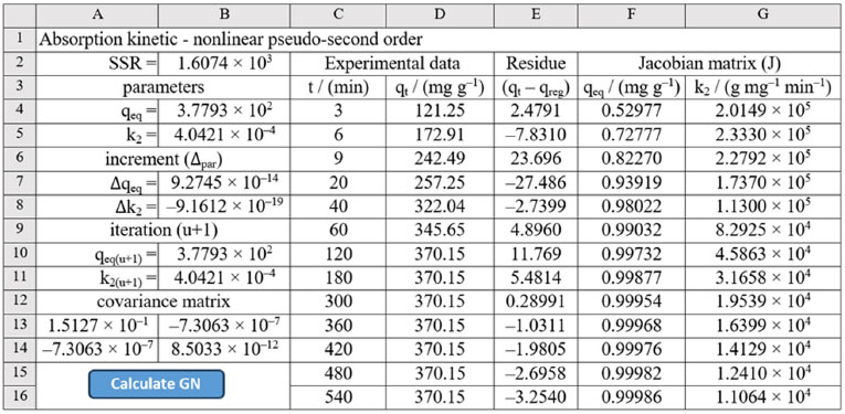
Figure 1 shows the layout of the ADSORB-XL Excel spreadsheet, illustrating the visual and structural organization of formatted cells. To obtain the desired parameters through simple nonlinear regression using the least squares method with the Gauss-Newton algorithm, several essential components are required: the column containing experimental data for the independent variables (range C4:C16); the column containing experimental data for the dependent variables (range D4:D16); the sum of squared errors or residuals (SSR), the value of which is calculated in cell B2 according to Equation 2 by multiplying the transpose of the residual vector by the residual vector, (R^T⋅R), using the Excel formula =MMULT(TRANSPOSE(E4:E16),E4:E16); the Jacobian matrix (derivative matrix) (range F4:G16); and finally, the parameter increments for each iteration (range B7:B8).

Figure 1
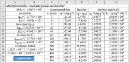
ADSORB-XL excel spreadsheet layout for nonlinear regression of pseudo-second order adsorption kinetics using experimental data from Silva et al.³⁴ SSR: sum of squared residuals (objective function minimized by the Gauss-Newton method); q_eq: value of the adsorption capacity optimized by the regression; k₂: value of the rate constant optimized by the regression; t: experimental contact time; q_t: experimental amount adsorbed at time t; residue (R): defined in the spreadsheet as the difference (q_t – q_reg), where q_reg is the value predicted by the model; Jacobian matrix: matrix containing the partial derivatives of the model with respect to q_eq and k₂; covariance matrix: used to determine the standard errors of the parameters

The parameter values, θ(u+1), are iteratively calculated using Equation 4, in which the updated values are obtained by adding those from the previous step, θ(u), to their respective increments. This process continues until the error falls within a predefined tolerance.

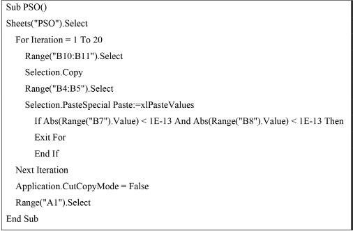
To automate the iterative process, users can record a simple macro that copies the values from the cell range (B10:B11) and pastes them as numerical values (without formatting) into the range (B4:B5). This process repeats until a defined stopping criterion is met, such as a specified number of iterations or a desired parameter precision (par), as shown in the spreadsheet illustrated in Figure 1. The resulting macro recording is low-complexity and the lines of Visual Basic for Applications (VBA) code required to execute this command, incorporating conditions like twenty iterations or a precision of 1 × 10^–13, are presented in Figure 2. Finally, a dedicated button can be assigned to run the newly created macro.

Figure 2
Macro with lines of code in VBA to automate the iteration process of nonlinear regression using the Gauss-Newton algorithm

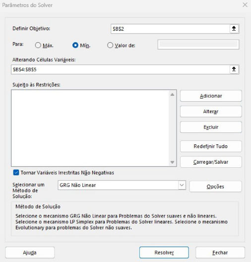
A simpler alternative for obtaining parameter values is to use the Solver add-in, which minimizes the sum of squared errors or residuals (SSR) (cell B2) by adjusting the parameter values in the range (B4:B5), Figure 3.

Figure 3
Solver supplemental tool for nonlinear regression

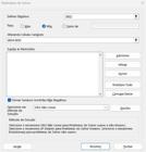
One advantage of using the Solver add-in for nonlinear regression via the least squares method is that it does not require the Jacobian matrix. Therefore, an Excel 365 (ADSORB-XL) spreadsheet can efficiently perform nonlinear regression using either the Gauss-Newton method or the Solver tool, achieving results comparable in speed and accuracy to specialized software such as Jupyter Notebook, RStudio, Matlab and Origin. Nonlinear regressions of both pseudo-second order adsorption kinetics and adsorption isotherm according to the Langmuir model are available in the Supplementary Material with lines of code following a step-by-step process.

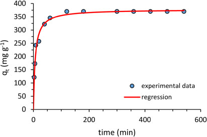
The graph illustrating the experimental data and the regression curve in Excel 365 for the pseudo-second order adsorption kinetics is shown in Figure 4.

Figure 4
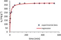
Pseudo-second order adsorption kinetics after nonlinear regression using experimental data for the SMF system at pH 5.5³⁴

Statistical analysis (regression and ANOVA) for the pseudo-second order adsorption kinetics was performed using equations from the literature,⁹,²⁷ and is presented in Table 3.

The experimental data fit to the pseudo-second order kinetic model was performed using simple nonlinear regression via the Gauss-Newton algorithm. The sum of squared residuals (SSR) was 1.6074 × 10³, resulting in a residual variance of 1.4613 × 10² and a residual standard deviation of 1.2088 × 10¹, considering 11 degrees of freedom (n = 13, p = 2). The determination coefficient (R²) of 0.98183 and the adjusted determination coefficient (R²_adj) of 0.98018 represent values considered robust for the kinetics of adsorptive processes. The F-test of the regression yielded F = 5.9437 × 102 (p = 6.3283 × 10^–11), indicating that the model is highly significant at a 95% confidence level.

In nonlinear regression, parameters are estimated through iterative methods to minimize the SSR, as no closed-form analytical solution exists. In this context, the covariance matrix is obtained through the expression:

(12) $\mathrm{Cov}(\text{θ})={\text{s}}^2{\left(J^{\text{T}}J\right)}^{-1}$

where J is the Jacobian matrix evaluated at the convergence point and s² is the estimated residual variance. Standard errors (SE) and confidence intervals (CI) are derived directly from this covariance matrix.

The estimated parameters were q_eq = 3.7793 × 10² mg g^–1 and k₂ = 4.0421 × 10^–4 g mg^–1 min^–1. The q_eq parameter exhibits higher statistical precision than the kinetic constant, a behavior expected for nonlinear kinetic models with asymptotic saturation. Standard errors were calculated from the square root of the diagonal elements of the covariance matrix, corresponding to SE(q_eq) = 4.7016 and SE(k₂) = 3.5250 × 10^–5.

The 95% confidence intervals were calculated using the SE values and the critical value of the Student’s t-distribution for 11 degrees of freedom (t_{0.025, 11} = 2.201), resulting in: q_max = 377.93 ± 10.35 mg g^–1, CI_95%(q_eq) = 367.58; 388.28, k₂ = (4.0421 ± 0.7759) × 10–4 g mg^–1 min^–1, CI_95%(k₂) = 3.2663 × 10–4; 4.8180 × 10–4.

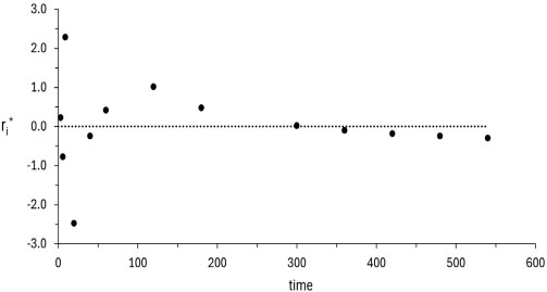
Residual analysis indicated an absence of systematic trends; standardized values are mostly within ± 2, and studentized residuals are compatible with the adopted confidence level (Figure 5). The sum of leverages was equal to the number of model parameters (∑h_ii = 2), confirming the mathematical consistency of the model, and no points with excessive influence were identified that could compromise parametric stability. Thus, the residual structure showed no evident heteroscedasticity or non-random behavior, corroborating the adequacy of the fit by the ordinary least squares method.

Figure 5
Studentized residuals - nonlinear regression of pseudo-second order adsorption kinetics using experimental data for the SMF system at pH 5.5

Diagnostic residual analysis can also reveal the presence of outliers (instrumental failure or gross experimental error), as these errors do not follow the predominant statistical pattern and can exert disproportionate influence on parameter estimation, rendering the fit unstable. Therefore, from a statistical standpoint, the model is adequate to describe the experimental data at a 95% confidence level.

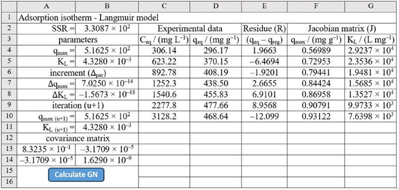
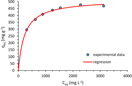
The nonlinear regression in ADSORB-XL for the Langmuir isotherm follows the same procedure as the pseudo-second order kinetic model, differing only in the experimental data and the model equation, as shown in Figures 6, 7 and Table 4.

Figure 6
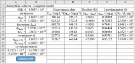
ADSORB-XL excel spreadsheet layout for nonlinear regression of the Langmuir adsorption isotherm (SMF system, pH 5.5). SSR: sum of squared residuals; C_eq: experimental equilibrium concentration; q_eq: experimental amount adsorbed at equilibrium; residue (R): difference between experimental and predicted values (q_eq – q_reg); q_max: maximum adsorption capacity for monolayer formation; K_L: Langmuir affinity constant; Jacobian matrix (J): partial derivatives of the Langmuir equation with respect to q_max and K_L; covariance matrix: provides the variance and covariance of the equilibrium parameters for error estimation

Figure 7
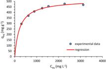
Langmuir adsorption isotherm with fitted curve after nonlinear regression (SMF system, pH 5.5)

Statistical analysis (regression and ANOVA) for the Langmuir isotherm (SMF system, pH 5.5) was performed using equations from the literature,¹⁰,³⁰,⁴¹ and is presented in Table 4.

The experimental data fit to the Langmuir model was performed using simple nonlinear regression via the Gauss-Newton algorithm. The sum of squared residuals (SSR) was 330.87, resulting in a residual variance of 66.174 and a residual standard deviation of 8.1347, considering 5 degrees of freedom (n = 7, p = 2).

It is observed that the q_max parameter exhibits higher relative precision, while the adsorption constant (K_L) shows greater uncertainty, a common behavior in nonlinear fits of adsorption isotherms, especially for experimental datasets with a limited number of points. The standard errors (SE) and 95% confidence intervals (CI) were estimated from the parameter covariance matrix calculated using Equation 12. The SE values were derived from the square root of the diagonal elements of the covariance matrix, corresponding to SE(q_max) = 7.4216 and SE(K_L) = 3.2833 × 10^–4.

The 95% confidence intervals were calculated using the critical value of the Student’s t-distribution for five degrees of freedom (t_{0.025, 5} = 2.571), resulting in: q_max = 516.25 ± 19.08 mg g^–1 and K_L = (4.3280 ± 0.8440) × 10^–3 L mg^–1.

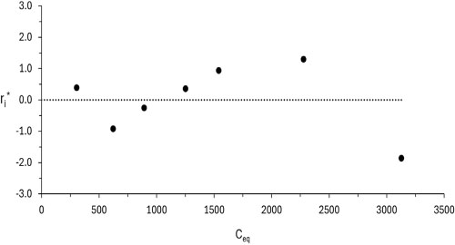
Studentized residual analysis indicated an absence of outliers at the 95% confidence level (|r_i^*| < 2.571) (Figure 8). The sum of leverages was equal to the number of model parameters (∑h_ii = 2), confirming the consistency of the hat matrix. Although the extreme data points exhibit higher leverage, as expected for the Langmuir model, no point exerted excessive influence over the estimated parameters. The residual standard error (s = 8.1347) represents approximately 2 to 3% of the experimental values, indicating an adequate fit. Overall, the statistical diagnostics indicate that the Langmuir model appropriately describes the experimental data, presenting statistically significant parameters and confidence intervals compatible with high experimental precision.

Figure 8
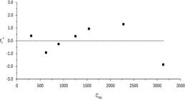
Studentized residuals - nonlinear regression of the adsorption isotherm according to the Langmuir model using experimental data for the SMF system at pH 5.5

The desktop version Microsoft Excel 365 is not free, but there is a free online version and a mobile version, both with fewer features. These free versions do not support macros or the Solver add-in, but if the nonlinear regression spreadsheet was built using the least squares method with the Gauss-Newton algorithm, it can be used across all versions without requiring programming skills.

Another great advantage of ADSORB-XL (Excel 365) is its ability to perform multiple nonlinear regressions for different models simultaneously within a single file, utilizing separate worksheets for each model.

The Supplementary Material was prepared with the objective of validating the calculations of nonlinear regressions of adsorption processes related to pseudo-first order kinetics, pseudo-second order kinetics and adsorption isotherm according to the Langmuir model in Excel 365 spreadsheets using the Jupyter Notebook, RStudio, Matlab and Origin software, providing the lines of code in the form of templates to be used in these software by changing only the experimental data in addition to instructions for using the “curve fitter tool” in Matlab and also the “nonlinear curve fit tool” in the Origin software to perform nonlinear regression.

In addition, the material enables users with no programming experience to reproduce nonlinear regression results while confirming the accuracy of the calculations performed in Excel 365.

Before evaluating the modeling results across the different platforms, it is worth noting that both the pseudo-second order (PSO) kinetic model and the Langmuir isotherm, which exhibited superior fits compared to other models, are widely utilized in adsorption studies. From a mechanistic perspective, pseudo-order models are simplifications that do not explicitly account for solvent resistance or diffusion, nor are they derived from detailed molecular mechanisms. Instead, they describe the adsorption rate as a function of the fraction of available sites, assuming that the rate-limiting step is the adsorption process itself. Similarly to the Langmuir model, they assume a homogeneous surface with equivalent adsorption sites.

Despite being a simplified approach, the PSO fit indicates that the adsorption rate is controlled by chemical interactions (chemisorption), likely due to the electrostatic attraction between the cationic MB molecules and the functional groups (such as carboxyl and hydroxyl groups) present on the surface of the activated carbons. The success of the Langmuir model further suggests that this interaction occurs through localized monolayer adsorption on a homogeneous surface, where each site accommodates a single MB molecule and there is no significant interaction between adjacent adsorbates.

In addition, the maximum adsorption capacities (q_max) and kinetic rate constants (k₂) calculated by ADSORB-XL are in excellent agreement with literature values.³⁴,³⁵ This consistency validates the reliability of the tool for processing real experimental datasets. In addition, no reproducibility issues were observed; all nonlinear regressions performed for the adsorption processes (kinetic and isotherm models) were reproducible across the five software platforms used (Excel, Jupyter Notebook, RStudio, Matlab, and Origin).

The results obtained from the nonlinear regressions for pseudo-second order kinetics and the Langmuir isotherm for the three samples SMF, TH and TS, using Excel 365, Jupyter Notebook, RStudio, Matlab and Origin are summarized and presented in Tables 5 to 10.

Significance of the statistical parameters in nonlinear regression

In a nonlinear regression analysis, some statistical parameters are important for assessing the quality and significance of the model fit to the data. This section details the parameters used in Figures 1 and 6, and Tables 3-10, as well as other widely used statistical parameters in nonlinear regression analyses, their importance and the formulas for calculation.

Parameters estimation (q_eq, k₂, q_max, K_L): the calculated parameters refer to the process of determining the numerical values of the model parameters (θ_i) that best fit the experimental data. In nonlinear regression, there are no predefined formulas to directly obtain parameter values from experimental data and the model equation. Therefore, in kinetic and isothermal adsorption studies, initial parameter estimates are typically obtained in three ways: (i) linearization of the model equation; (ii) solving systems of equations, and (iii) graphical methods.

Once an initial estimate of the parameter values is obtained using one of these methods, these values serve as starting points for the iterative process. Good initial values lead to rapid convergence and help avoid local minimum. In this study, the initial parameters values for the iterative process were derived from the linearization of the models. The nonlinear regressions were performed using the least squares method with the Gauss-Newton algorithm.

Coefficient of determination (R²)

This is a statistical measure that indicates how well the regression model explains the variability of the observed data.⁴¹ An R² value close to 1 suggests a better fit, allowing for comparisons between different regression models to determine the best representation of the data. R² is calculated using Equation 13.

(13) ${\text{R}}^2=1-\frac{\text{SSR}}{\text{SST}}$

where: SSR is the sum of squared residuals (sum of squared differences between observed and predicted values, Equation 14), and SST is the total sum of squares (sum of the squared differences between observed and average values, Equation 15).

(14) $\text{SSR}={\displaystyle \sum {\left({\text{y}}_{\text{i}}-{\hat{\text{y}}}_{\text{i}}\right)}^2}$

(15) $\text{SST}={\displaystyle \sum {\left({\text{y}}_{\text{i}}-{\bar{\text{y}}}_{\text{i}}\right)}^2}$

Concerning the observed R² values for the experimental results presented in this study, with exception of the R² values obtained from the nonlinear regression of the pseudo-second order kinetics and adsorption isotherm for the TS sample (R² = 0.857 and 0.915, respectively), all others R² values for SMF and TH samples were greater than 0.98. This indicates that the models used in the nonlinear regressions explain nearly all the variance of the data.⁴¹

Adjusted coefficient of determination (R²_adj)

This parameter is a refined version of R² that accounts for the number of model parameters, helping to prevent overfitting by applying a penalty to unnecessary variables. This adjustment makes R²_adj particularly useful for comparing models with different parameter counts, such as adsorption isotherms like the Langmuir (2 parameters), Sips (3 parameters), and Fritz (4 parameters) models. The adjusted coefficient of determination (Equation 16) is calculated as:

(16) ${\text{R}}_{\text{adj}}^2=1-\left(1-{\text{R}}^2\right)\frac{(\text{n}-1)}{(\text{n}-\text{p})}$

where R² is the coefficient of determination, n is the number of observations and p is the number of model parameters.

Standard error of estimate or standard error of regression (Se)

Standard error (Se) value quantifies the dispersion of observed values around the regression line, providing a measure of the accuracy of the predictions of the model. A lower Se indicates that the observed values are closer to the regression line, meaning the model provides more precise predictions.

The standard error of the estimate is given by Equation 17, where df_res (degree of freedom for residuals) is the number of observations (n) minus the number of model parameters (p) (Equation 18).

(17) $\text{Se}=\sqrt{\frac{\text{SSR}}{{\text{df}}_{\text{res}}}}$

(18) ${\text{df}}_{\text{res}}=\text{n}-\text{p}$

Regarding the Se values obtained from the nonlinear regressions of the SMF, TS, and TH samples, their small magnitudes indicate a limited dispersion of the observed data points around the predicted regression lines. This suggests that the models provide adequate fit for each of the investigated samples.

Analysis of variance (ANOVA)

ANOVA is a statistical method used to assess the variability in a regression model by comparing different sources of variation. The ANOVA table typically includes degrees of freedom (df), sum of squares (SS), mean square (MS), F-statistic (F), and F-significance (p-value). In addition to Equation 17 for the degrees of freedom for residuals (df_res), the degrees of freedom for regression (df_reg) and total (df_tot) can be calculated using the Equations 19 and 20.

(19) ${\text{df}}_{\text{reg}}=\text{n}-\text{p}$

(20) ${\text{df}}_{\text{tot}}=\text{n}-1$

The sum of squares (SS) is also calculated for different sources of variation (regression, residual, and total). The sum of squares of the residuals (SSR) and total sum of squares (SST) have been previously defined (Equations 13 and 14, respectively). The regression sum of squares (SS_Reg) is the difference between the total sum of squares and the sum of squares of the residuals, as expressed by Equation 21.

(21) ${\text{SS}}_{\text{reg}}=\text{SST}-\text{SSR}$

A lower SSR relative to SST indicates a better model fit. As observed in this study, all regressions minimized SSR, confirming the convergence of the iterative method.

The mean square (MS) is also calculated for different sources of variation, specifically regression (MS_reg) and residuals (MSR). These calculations, given by Equations 22 and 23, respectively, serve as the basis for determining the F-statistic and its associated p-value (F-significance).

(22) $\text{MSR}=\frac{\text{SSR}}{{\text{df}}_{\text{res}}}$

(23) $\text{MSR}=\frac{\text{SSR}}{{\text{df}}_{\text{res}}}$

F-Statistic and significance (p-value)

The F-statistic measures the ratio of the variance explained by the model to the variance remaining unexplained, helping to assess the overall significance of the regression. It is calculated by Equation 24:

(24) $\text{F}=\frac{{\text{MS}}_{\text{Reg}}}{\text{MSR}}$

The p-value (also referred to as F-significance)

F-significance is derived from the F-statistic and its respective degrees of freedom, representing the probability of obtaining an F-statistic as extreme as the observed one under the null hypothesis. A p-value < 0.05 indicates that the coefficients of the model are statistically significant.

The ADSORB-XL tool implements the FDIST(F, df_reg, df_res) function to compute F-statistic significance values. Across all nonlinear regression analyses performed in this investigation, the obtained F-significance values remained consistently below the 5% threshold (p < 0.05), thereby statistically validating all applied adsorption models at a 95% confidence level.

Statistical analysis of parameters

Standard error of parameters, Se(θ_i)

The standard error of parameters measures the variability of parameter estimates, indicating the precision of the calculated values – lower standard errors mean greater precision. It is calculated by Equation 25.

(25) $\text{Se}\left({\text{θ}}_{\text{i}}\right)=\sqrt{\text{MSR}\times {\text{a}}_{\text{ij}}}$

where: a_ij represents the elements of the main diagonal of the variance-covariance matrix.

Se(θ_i) are also used to determine the statistical significance of coefficients in t-Stat, p-value calculations and in determining the confidence interval.

As anticipated, the standard error values (Se) for each regression performed in this work showed consistency when compared between the different software platforms employed.

t-Statistic or t-Stat

The t-statistic is a test of the statistical significance of individual model parameters, indicating whether they significantly contribute to the model. It is calculated as:

(26) $t-\text{Stat}=\frac{{\text{θ}}_{\text{i}}}{\text{Se}\left({\text{θ}}_{\text{i}}\right)}$

The t-statistic values for the parameters of each regression in this study were in agreement with those computed using Excel (ADSORB-XL), Jupyter Notebook, RStudio, Matlab and Origin software. Origin software facilitates manual calculation so the parameter estimates and their corresponding standard errors are presented in Tables 5 to 10 and in the Supplementary Material.

p-Value

The p-value is the probability that the observed results arose by random variation, and is used to evaluate the statistical significance of estimated parameters. A p-value below 0.05 is generally considered to indicate statistical significance. It is derived from the two-tailed Student’s t-distribution (or the normal distribution for large samples), using the t-statistic (t-Stat) and the residual degrees of freedom (df_res). The p-value solely reflects the statistical significance of the parameters, not the size of their effects. Consequently, a small p-value (p < 0.05) suggests that the observed result is unlikely due to chance alone, supporting the conclusion that the parameter is statistically significant.

Microsoft Excel 365 (ADSORB-XL) provides the function T.DIST (t-Stat, df_res, 2) to compute the probability of the two-tailed Student’s t-distribution, utilizing the t-statistic and the residual degrees of freedom as inputs.

Across all regressions conducted in this study, the obtained p-values were below the significance level of 0.05 (5%), thus demonstrating the statistical significance of the employed models.

Confidence interval (CI)

The confidence interval defines a range within which the true parameter value is expected to lie with a given confidence level (e.g., 95%). It is calculated using Equation 27:

(27) $\text{CI}={\text{θ}}_{\text{i}}\pm {\text{t}}_{\text{C}}\times \text{Se}\left({\text{θ}}_{\text{i}}\right)$

where t_C is the critical value from the t-distribution, determined using the two-tailed Student’s t-distribution (or the normal distribution if the sample size is large). This value depends on the chosen confidence level (e.g. 95%) and the residual degrees of freedom (df_res). In Microsoft Excel 365 (ADSORB-XL), t_C can be obtained using the T.INV(0.05, df_res) function for a 95% confidence level or 5% significance.

Formulas in Microsoft Excel 365 vary depending on the language and operating system settings, as well as the delimiters. Therefore, it is important to be careful to avoid calculation errors.

CONCLUSIONS

When selecting software for nonlinear regression of adsorption data, accessibility and ease of use are critical factors. While some programs provide intuitive interfaces, others require proficiency in programming.

When comparing ADSORB-XL, a spreadsheet developed in Excel 365 for nonlinear regression analysis in adsorption processes, with four widely used academic platforms (Jupyter Notebook, RStudio, Matlab and Origin), it was found that their mathematical modeling capabilities are equivalent. The tool demonstrated similar accuracy in fitting experimental data to adsorption models, as evidenced by the excellent agreement between the parameter values obtained across all platforms. This performance equivalence confirms ADSORB-XL as a statistically robust alternative for adsorption studies, combining analytical reliability with the accessibility advantages of spreadsheet-based computing.

ADSORB-XL, with its intuitive tools and user-friendly interface, proved particularly suitable for users without specialized programming knowledge. In contrast, RStudio, Jupyter Notebook, and Matlab, while more complex in their learning curve, offer greater flexibility and a more robust set of tools for advanced statistical analysis, allowing for customization and the development of scripts for specific tasks.

The results of this study show that the choice of the most suitable software should take into account not only the accuracy of the fits, but also user familiarity with the interface and the programming language. Accessible tools such as ADSORB-XL, which provide nonlinear regression and statistical analysis capabilities, help democratize access to advanced methods, particularly for professionals and researchers without extensive programming skills.

SUPPLEMENTARY MATERIAL

Complementary material for this work is available at http://quimicanova.sbq.org.br/, as a file, with free access.

Supplementary PDF

Supplementary PDF

DATA AVAILABILITY STATEMENT

All data generated or analyzed during this study are included in this published article and its supplementary information files. Any additional data may be obtained from the corresponding authors upon reasonable request.

ACKNOWLEDGMENTS

The authors would like to thank the Postgraduate Program in Chemistry at IFMA and the Study Group on Inorganic and Catalysis.

REFERENCES

• ¹ Dabrowski, A.; Adv. Colloid Interface Sci. 2001, 93, 135. [Crossref]
  » Crossref
• ² Foo, K. Y.; Hameed, B. H.; Chem. Eng. J. 2010, 156, 2. [Crossref]
  » Crossref
• ³ Nascimento, R. F.; Lima, A. C. A.; Vidal, C. B.; Oliveira, A. G.; Melo, D. Q.; Adsorção: Aspectos Teóricos e Aplicações Ambientais, 2a ed.; Imprensa Universitária: Fortaleza, 2020. [Link] accessed in March 2026
  » Link
• ⁴ Mendonça, J. C.; Cantanhede, L. B.; Rojas, M. O. A. I.; Rangel, J. H. G.; Bezerra, C. W. B.; Water Supply 2022, 22, 481. [Crossref]
  » Crossref
• ⁵ Zheng, X.; Alam, O.; Zhou, Y.; Du, D.; Li, G.; Zhu, W.; J. Environ. Chem. Eng. 2024, 12, 114366. [Crossref]
  » Crossref
• ⁶ Adeoye, J. B.; Lau, S. Y.; Tan, Y. H.; Discover Appl. Sci. 2025, 7, 1285. [Crossref]
  » Crossref
• ⁷ Somashekara, D.; Lavanya, M. N.; ChemBioEng Rev. 2023, 10, 828. [Crossref]
  » Crossref
• ⁸ Tran, H. N.; You, S. J.; Hosseini-Bandegharaei, A.; Chao, H. P.; Water Res. 2017, 120, 88. [Crossref]
  » Crossref
• ⁹ Wang, M.; Xue, Y.; Du, J.; J. Chem. Phys. 2023, 159, 234106. [Crossref]
  » Crossref
• ¹⁰ Lima, E. C.; Adebayo, M. A.; Machado, F. M. In Carbon Nanomaterials as Adsorbents for Environmental and Biological Applications; Bergmann, C. P.; Machado, F. M., eds.; Springer: Cham, 2015, ch. 3. [Crossref]
  » Crossref
• ¹¹ Bates, D. M.; Watts, D. G.; Nonlinear Regression Analysis and Its Applications; Wiley: New York, 1988. [Crossref]
  » Crossref
• ¹² Klug, M.; Sanches, M. N. M.; Laranjeira, M. C. M.; Fávere, V. T.; Rodrigues, C. A.; Quim. Nova 1998, 21, 410. [Link] accessed in March 2026
  » Link
• ¹³ Brown, A. M.; Computer Methods and Programs in Biomedicine 2001, 65, 191. [Crossref]
  » Crossref
• ¹⁴ Vitek, R.; Masini, J. C.; Heliyon 2023, 9, e15128. [Crossref]
  » Crossref
• ¹⁵ Beck, A.; Introduction to Nonlinear Optimization: Theory, Algorithms, and Applications with Python and Matlab, 2nd ed.; SIAM: Philadelphia, 2023. [Crossref]
  » Crossref
• ¹⁶ Massaron, L.; Boschetti, A.; Regression Analysis with Python; Packt Publishing: Birmingham, 2016.
• ¹⁷ Del Toro, I.; Dickson, K.; Hakes, A. S.; Newman, S. L.; The American Biology Teacher 2022, 84, 124. [Crossref]
  » Crossref
• ¹⁸ Mazucheli, J.; Achcar, J. A.; Acta Sci., Technol. 2002, 24, 1761. [Crossref]
  » Crossref
• ¹⁹ da Fonseca, J. A.; Research, Society and Development 2022, 11, e212111226071. [Crossref]
  » Crossref
• ²⁰ Silva, E. M.; Fruhauf, A. C.; Fernandes, F. A.; de Paula, G. S.; Muniz, J. A.; Fernandes, T. J.; Sigmae 2019, 8, 728. [Crossref]
  » Crossref
• ²¹ dos Santos, C. C.; Mouta, R.; Castro Junior, M. C.; Santana, S. A. A.; Silva, H. A. S.; Bezerra, C. W. B.; Carbohydr. Polym. 2018, 180, 182. [Crossref]
  » Crossref
• ²² Ferreira, A. S.; Mota, A. A.; Oliveira, A. M.; Rodrigues, F. I. L.; Pacífico, S. N.; Silva, J. E.; Abagaro, B. T. O.; Saraiva, G. D.; Castro, A. J. R.; Teixeira, R. N. P.; Sousa Neto, V. O.; Rev. Virtual Quim. 2019, 11, 1480. [Crossref]
  » Crossref
• ²³ Teymourifar, A.; Heliyon 2023, 9, e18602. [Crossref]
  » Crossref
• ²⁴ Altiok, E.; Mahfuz, M.; Karadeniz Fen Bilimleri Dergisi 2024, 14, 2069. [Crossref]
  » Crossref
• ²⁵ Pine, D. J.; Introduction to Python for Science and Engineering; CRC Press: Boca Raton, 2019.
• ²⁶ Craig, P. A.; Nash, J. A.; Crawford, T. D.; Biochem. Mol. Biol. Educ. 2022, 50, 479. [Crossref]
  » Crossref
• ²⁷ Edwards, P. M.; J. Chem. Inf. Model. 2002, 42, 1270. [Crossref]
  » Crossref
• ²⁸ Venkataraman, P.; Applied Optimization with Matlab Programming, 2nd ed.; John Wiley: Hoboken, 2009.
• ²⁹ Hunt, B. R.; Lipsman, R. L.; Rosenberg, J. M.; A Guide to Matlab, 3rd ed.; Cambridge University Press: Cambridge, 2014.
• ³⁰ Mustafy, T.; Rahman, Md. T. U.; Statistics and Data Analysis for Engineers and Scientists, 1st ed.; Springer: Singapore, 2024. [Crossref]
  » Crossref
• ³¹ Süli, E.; Mayers, D. F.; An Introduction to Numerical Analysis; Cambridge University Press: Cambridge, 2011.
• ³² Siregar, R. W.; Tulus; Ramli, M.; IOP Conf. Ser.: Mater. Sci. Eng. 2018, 300, 012044. [Crossref]
  » Crossref
• ³³ Lai, W. H.; Kek, S. L.; Tay, K. G.; International Journal of Innovative Science, Engineering & Technology 2017, 4, 258. [Link] accessed in March 2026
  » Link
• ³⁴ Silva, F. A.; Cantanhede, L. B.; Marques, I. S.; de Figueredo, G. P.; Quim. Nova 2024, 47, e20230106. [Crossref]
  » Crossref
• ³⁵ Pinheiro, V. L. F.: Adsorção de Azul de Metileno Utilizando Carvão Preparado a Partir da Casca do Tamarindo (Tamarindus Indica L.) e Tratado com Ozônio; Dissertação de Mestrado, Instituto Federal do Maranhão, São Luís, Brasil, 2024. [Link] accessed in April 2026
  » Link
• ³⁶ Rubin, S. J.; Abrams, B.; J. Chem. Educ. 2015, 92, 1840. [Crossref]
  » Crossref
• ³⁷ Hair, J. F.; Hult, G. T. M.; Ringle, C. M.; Sarstedt, M.; Danks, N. P.; Ray, S.; A Primer on Partial Least Squares Structural Equation Modeling (PLS-SEM), 3rd ed.; Springer: Cham, 2021. [Crossref]
  » Crossref
• ³⁸ Martinez, W. L.; Martinez, A. R.; Exploratory Data Analysis with Matlab®; Chapman & Hall/CRC: London, 2004.
• ³⁹ May, R. A.; Stevenson, K. J.; J. Am. Chem. Soc. 2009, 131, 872. [Crossref]
  » Crossref
• ⁴⁰ Deschenes, L. A.; Vanden Bout, D. A.; J. Am. Chem. Soc. 2000, 122, 9567. [Crossref]
  » Crossref
• ⁴¹ Miller, J. C.; Statistics for Analytical Chemistry, 3rd ed.; Ellis Horwood: New York, 1993.

Editado por

• Executive Editor handled this article: Gustavo F. S. Andrade

Datas de Publicação

• Publicação nesta coleção
  12 Jun 2026
• Data do Fascículo
  2026

Histórico

• Recebido
  05 Dez 2025
• Aceito
  18 Mar 2026
• Publicado
  27 Abr 2026