
Abstract
The integral form of the fourth Maxwell’s equation is often written in two different ways: in the first, the partial derivative of Electric field appears, while the second contains a time derivative of electric flux integral. It would be useful, from a didactic point of view, to discriminate between the two different interpretations. In this paper, starting from a previous work about Faraday’s law, we analyze the derivative of the flux of the electric field and we shed light on the right way to write the Maxwell equations. We introduce a “magnetomotive force” and we find, from the corresponding generalization of the second Laplace’s law, the effect of a rotation induced in a coil embedded in an electric field.
Keywords
Maxwell equations; Displacement current
1. Introduction
By reading many textbooks for undergraduate and advanced students, we have found a sort of ambiguity in the integral form of the fourth Maxwell’s equation that can be written in a first version as [11. L. Landau and E. Lifsits, Classical Theory of Fields (London, Pergamon, 1971), 3a ed., 22. J.D. Griffiths, Introduction to Electrodynamics (Cambridge University Press, 2017), 4a ed.]
and in a second version as [33. P. Tipler, Physics for Scientists and Engineers (W. H. Freeman and Company, New York, 1998), 4a ed., 44. M. Alonso and E.J. Finn, Fundamental University Physics: vol. 2 Fields and waves (Addison Wesley Publishing Company, Boston, 1968), 2a ed., 55. R.A. Serway and J.W. Jewett, Physics for Scientists and Engineers (Brooks/Cole Publishing Company, Pacific Grove, 2012), 9a ed., 66. D. Giancoli, Physics: Principles with Applications (Pearson Higher Education, London, 2015)., 77. D. Halliday, R. Resnick and J. Walker, Fundamentals of Physics (John Wiley & Sons, Hoboken, 2013), 10a ed., 88. D. Fleisch, A Student’s Guide to Maxwell’s Equations (Cambridge University Press, Cambridge, 2008)., 99. J.A. Stratton, Electromagnetic Theory (McGraw Hill, New York, 1941).]
and, of course, only one of the two equations has to be right. It is worth noting that the two equations are equivalent if in the flux ΦE only the electric field depends on time, and that the presence of the time derivative of the flux of electric field in the second equation makes it more similar to the Faraday’s law and allows to express the Maxwell’s equations in a more symmetrical and elegant way. From a theoretical point of view, we observe that, in order to obtain the standard Maxwell equation in differential form,
the first version (1) is mathematically right, while if the displacement current depends on the derivative of the flux, as in (2), it is necessary to modify the relation and to study the physical consequences of the corrections.
All the difference between the two equations depends on the term containing the flux and if we have a flux integral
it is well known, from mathematical analysis, that it is possible to calculate its time derivative. The derivative of the flux integral is of great importance in physics. In fact, for example, if the vector field is the magnetic one, the derivative of the flux generates an electromotive force such that
where S(t) is a surface that has a circuit l as its boundary. The integral form of Faraday’s law refers to two phenomena. A current can be induced in a coil either by variation in time of the magnetic field in which the circuit is embedded or by a relative velocity between the coil and the field. The first effect leads to the third Maxwell’s equation, the second is linked to the Lorentz force [1010. R.P. Feynman, R.B. Leighton and M. Sand, Feynman lectures on Physics (Addison-Wesley, Boston, 1964), v. 2., 1111. J.D. Jackson, Classical Electrodynamics (John Wiley & Sons, New York 1975), 2a ed., 1212. A. Pramanik, Electromagnetism: Theory and Applications (PHI Learning, New Delhi, 2004)., 1313. L. Chow, Introduction to electromagnetic theory: a modern perspective (Jones & Bartlett Learning, Burlington, 2006).]. The standard notation, which clearly explains the two contributions, is the following
Although the electromagnetic induction has been well known for more than 150 years, it still requires reflections in teaching perspective and, over the years, many papers have been written to describe it in the most general case [1414. H. Flanders, The American Mathematical Monthly 80, 615 (1973)., 1515. P.J. Scanlon, R.N. Henriksen and J.R. Allen, American Journal of Physics 37, 698 (1969)., 1616. H. Gamo, Proceedings of the Ieee 67, 676 (1979)., 1717. N. Rosen and D. Schieber, American Journal of Physics, 50, 974 (1982)., 1818. H. Gelman, European Journal of Physics 12, 230 (1991)., 1919. F. Munley, American Journal of Physics 72, 1478 (2004)., 2020. D.V. Redzic, European Journal of Physics 28, N7 (2007)., 2121. D.V. Redzic, European Journal of Physics 29, L5 (2008)., 2222. A. Lopez-Ramos, J.R. Menendez and C. Piquè, European Journal of Physics 29, 1069 (2008)., 2323. E. Benedetto, Afr. Mat. 28, 23 (2017).]. In a previous article [2424. E. Benedetto, M. Capriolo, A. Feoli and D. Tucci, European Journal of Physics 33, L15 (2012).], we have considered the evolution of a circuit, simultaneously embedded in a changing magnetic field, and enlarging its length from a time t to a time t + Δt, showing the validity of the previous relation (6) in this more general case and the necessity to introduce a more precise definition of electromotive force with respect to what is generally found in textbooks. Now we want to follow a similar reasoning but considering the same enlarging circuit, where a current passes, embedded in a varying electric field. In this way, we show that, to recover the fourth Maxwell’s equation, it is necessary to introduce a magnetomotive force that is a generalization of the one present in literature. The paper is organized as follows: in Section 2 2. Flux Time Derivative We consider the same case studied in [24], but this time the coil, where a current i passes, is immersed in an electric field E→ and not in a magnetic field. We repeat the same calculations made in that paper but with B→ substituted by E→. Hence we start analyzing the following integral function (7) Φ E ( t ) = ∬ S ( t ) E → ( t , r → ( t ) ) ⋅ n ^ d S . Now we look at Fig. 1 of [24] and calculate the derivative Figure 1 A circuit in which a current I flows and we have put our small coil (in red) in the space between the two plates of the capacitor embedded in a region of electric field E→ and moving with velocity v→ from the position S(t) to the position S(t + Δt). (8) d Φ E d t = lim Δ t → 0 ∬ S ( t + Δ t ) E → ( t + Δ t , r → ( t + Δ t ) ) ⋅ n ^ d S - ∬ S ( t ) E → ( t , r → ( t ) ) ⋅ n ^ d S Δ t , and, considering the closed surface σ formed by S(t), S(t + Δt) and the lateral surface Σ, at the fixed instant t + Δt, we assume that there is no internal charge and therefore ∇→⋅E→=0 or in integral form (9) Φ σ = ∫ σ ∫ ○ E → ⋅ n ^ d S = 0 . Then we can compute the derivative of the integral function using the definition of equation (8). The result is the same as equation (13) of [24] (obtained neglecting terms of second order in the Taylor expansions), with B→ substituted by E→ (10) d Φ E ( t ) d t = ∬ ( S ( t ) ) ( ∂ E → ∂ t ) ⋅ n ^ d S - ∮ ( ∂ C ) ( v → × E → ) ⋅ d l → . We insert this flux in the integral form of the Maxwell’s equation (2) and consider the case in Fig. 1 of a circuit in which a current I flows. The first term on the right side of equation appears if the surface S(t) is linked to the wire, the second term is non vanishing when the surface S(t) is between the plates of the capacitor. We put our small coil just in the space between the two plates, but in the general case we have (11) ∮ ( ∂ C ) B → ⋅ d l → = μ 0 I + ε 0 μ 0 [ ∬ ( S ( t ) ) ( ∂ E → ∂ t ) ⋅ n ^ d S - ∮ ( ∂ C ) ( v → × E → ) ⋅ d l → ] . From this equation we cannot obtain the right fourth Maxwell’s equation (3) For this reason it is legitimate to define a sort of generalized “magnetomotive force” (12) f B = ∮ ( ∂ C ) ( B → - v → c 2 × E → ) ⋅ d l → , such that (13) ∮ ( ∂ C ) B → ⋅ d l → - 1 c 2 ∮ ( ∂ C ) ( v → × E → ) ⋅ d l → = ε 0 μ 0 ∬ ( S ) ∂ E → ∂ t ⋅ n ^ d S - 1 c 2 ∮ ( ∂ C ) ( v → × E → ) ⋅ d l → + μ 0 I , that is, neglecting terms of second order in Taylor expansion [24], (14) ∮ ( ∂ C ) B → ⋅ d l → - 1 c 2 ∮ ( ∂ C ) ( v → × E → ) ⋅ d l → = ε 0 μ 0 d Φ E d t + μ 0 I , that leads to the right Maxwell’s equation in differential form (3). Hence we have shown that, if one wants to express the Maxwell’s equation in terms of flux, the integral form (2) must be modified and substituted by the equation (14). Now that we have corrected the equation (2), we argue that equations (1) and (14) are two ways to write the same equation leading to the same differential equation (3). In order to obtain the equation (13) and then (14), we have had to change the left side of the equation not in a casual way, but operating a precise transformation of the magnetic field. Actually, we can show that the equation (2) (directly related to the equation (14)) can be obtained from the equation (1) applying to the electric and magnetic fields a Lorentz transformation (see Appendix). Hence the equation (14) makes only more explicit the case in which there is the movement of charges with respect to the fields or viceversa. But equation (14) appears more useful also because it allows a clear interpretation in terms of forces acting on charges. Note that in literature different definitions of magnetomotive force can be found. Among them the closest to our definition is (15) 𝔉 B = ∮ ( ∂ C ) H → ⋅ d l → = ∮ ( ∂ C ) B → μ 0 ⋅ d l → . In analogy with the definition of the electromotive force, we can interpret the magnetomotive force as the ratio between the work L in a closed circuit and the magnetic charge qB just as it occurs in the theory of magnetic monopoles [25, 26], where there are two similar expressions of forces acting on electric and magnetic charges respectively: (16) F → E = q E ( E → + v → × B → ) , (17) F → B = q B ( B → - v → c 2 × E → ) . From which we can define (18) f E = L q E = 1 q E ∮ ( ∂ C ) F E → ⋅ d l → , (19) f B = L q B = 1 q B ∮ ( ∂ C ) F B → ⋅ d l → . Therefore, we can write the flux rule equations in an appealing and symmetrical way (20) f E = - d Φ B d t , and (21) f B = μ 0 I + ε 0 μ 0 d Φ E d t , that have the advantage to include in the integral form of Maxwell’s equations also the expressions of the forces (16) and (17). From the Ampere’s equivalence theorem, the forces and the momenta experienced by the magnetic charges of a magnetic dipole, are the same that act on an element of current idl→ of a small loop, hence we can obtain from (17) the following generalization of the second Laplace’s formula (see also the appendix) (22) d F → = i d l → × ( B → - v → c 2 × E → ) , that we can apply to a coil immersed in an electric field E→ and in which a current i passes. , following [2424. E. Benedetto, M. Capriolo, A. Feoli and D. Tucci, European Journal of Physics 33, L15 (2012).], we analyze the derivative of the flux of the electric field introducing the “magnetomotive force”; Section 3 3. Flux Cutting We apply the considerations of the previous section to the case of a rectangular coil embedded in a constant electric field (Fig. 2). The example we choose is the analog of the well known exercise, studied in all the didactic textbooks for a coil in a magnetic field, in the chapter of Flux cutting for Faraday’s law and a similar example was also examined in ref. [27], but without obtaining the result of the rotation of the coil. Figure 2 A rectangular coil (in blue) embedded in a region (with dashed border) of electric field E→ and moving to the right with velocity v→. At the initial time the coil moves with a constant velocity v→, beginning to go out of the region where the field is present. A current flows into the wire of the coil in the counterclockwise direction. Looking at Fig. 2, we have E→=|E→|x^, v→=|v→|y^, dl1→=|dl1→|y^, dl2→=|dl2→|z^, and the Laplace’s formula (22), neglecting the magnetic field generated by the current of the coil itself (B→=0), becomes (23) d F → = - i d l → × ( v → c 2 × E → ) . In our case v→×E→=-|v→||E→|z^ getting (24) { d F → 1 = - i d l → 1 × ( v → c 2 × E → ) = i | d l → 1 | | v → | | E → | c 2 x ^ d F → 2 = - i d l → 2 × ( v → c 2 × E → ) = 0 . Therefore (25) F → B G = i B G ( t ) | v → | | E → | c 2 x ^ = - F → A H . These two forces generate a rotation of the coil around an axis parallel to the side BC, with a momentum given by the second fundamental law of mechanics (26) | τ → | = | F → | b = I i n d ω d t , where b is the distance between the two forces and Iin is the moment of inertia of the coil. We can write (27) i B G ( t ) | v → | | E → | c 2 ( A B ) = 1 12 M ( A B ) 2 d ω d t , getting (28) d ω d t = 12 i B G ( t ) | v → | | E → | M ( A B ) c 2 = 12 i | v → | | E → | M ( A B ) c 2 ( B C - | v → | t ) , where M is the mass of the coil. In the case the electric field is due to a capacitor, with a surface charge density σ, and the coil is a square of side ℓ instead of a rectangle, we can write: (29) d ω d t = 12 i | v → | σ M ϵ 0 c 2 ( 1 - | v → | t ℓ ) . The angular velocity is: (30) ω ( t ) = 12 i | v → | σ M ϵ 0 c 2 t ( 1 - | v → | t 2 ℓ ) . At this point, it would be very useful to describe in details an experimental apparatus to verify the existence of the rotation effect. This project goes beyond the scope of the present paper, however we can at least give an estimate of the angular velocity after one second using some effective values of the parameters appearing in (30). Substituting M = 0.1 Kg, σ = 0.1 C/m2, |v→|=0.1 m/s, ℓ = 0.3 m, i=3 A, t=1 sec, in the equation (30), the result is ω = 1.1×10⁻⁵rad/sec. is devoted to the application of a generalized second Laplace’s law to the case of Flux cutting and, finally, in Section 4 4. Conclusions We have found in many textbooks two different ways (equations (1) and (2)) to write the integral form of the fourth Maxwell’s equation. We have shown that it is necessary to modify the relation (2) if we want to recover the standard Maxwell differential equation (3). The resulting equation (14) is correct and is related to the equation (1) by a Lorentz transformation. The equation (14) leads immediately to a corresponding generalization of the second Laplace’s formula. In this framework, we have studied the motion of a small loop of current outgoing from the region of an electric field and we have found that the coil must undergo a rotation. We have explicitly calculated the momentum of the forces for this rotation in the case of a rectangular loop and the angular velocity as a function of time. The result is that, in the case of flux cutting, as a current is induced in a coil moving with respect to magnetic force lines, so a rotation is induced in a coil moving with respect to electric force lines. there are the conclusions.
2. Flux Time Derivative
We consider the same case studied in [2424. E. Benedetto, M. Capriolo, A. Feoli and D. Tucci, European Journal of Physics 33, L15 (2012).], but this time the coil, where a current i passes, is immersed in an electric field and not in a magnetic field. We repeat the same calculations made in that paper but with substituted by . Hence we start analyzing the following integral function
Now we look at Fig. 1 of [2424. E. Benedetto, M. Capriolo, A. Feoli and D. Tucci, European Journal of Physics 33, L15 (2012).] and calculate the derivative
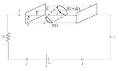
A circuit in which a current I flows and we have put our small coil (in red) in the space between the two plates of the capacitor embedded in a region of electric field and moving with velocity from the position S(t) to the position S(t + Δt).
and, considering the closed surface σ formed by S(t), S(t + Δt) and the lateral surface Σ, at the fixed instant t + Δt, we assume that there is no internal charge and therefore or in integral form
Then we can compute the derivative of the integral function using the definition of equation (8). The result is the same as equation (13) of [2424. E. Benedetto, M. Capriolo, A. Feoli and D. Tucci, European Journal of Physics 33, L15 (2012).] (obtained neglecting terms of second order in the Taylor expansions), with substituted by
We insert this flux in the integral form of the Maxwell’s equation (2) and consider the case in Fig. 1 of a circuit in which a current I flows. The first term on the right side of equation appears if the surface S(t) is linked to the wire, the second term is non vanishing when the surface S(t) is between the plates of the capacitor. We put our small coil just in the space between the two plates, but in the general case we have
From this equation we cannot obtain the right fourth Maxwell’s equation (3)
For this reason it is legitimate to define a sort of generalized “magnetomotive force”
such that
that is, neglecting terms of second order in Taylor expansion [2424. E. Benedetto, M. Capriolo, A. Feoli and D. Tucci, European Journal of Physics 33, L15 (2012).],
that leads to the right Maxwell’s equation in differential form (3). Hence we have shown that, if one wants to express the Maxwell’s equation in terms of flux, the integral form (2) must be modified and substituted by the equation (14). Now that we have corrected the equation (2), we argue that equations (1) and (14) are two ways to write the same equation leading to the same differential equation (3). In order to obtain the equation (13) and then (14), we have had to change the left side of the equation not in a casual way, but operating a precise transformation of the magnetic field. Actually, we can show that the equation (2) (directly related to the equation (14)) can be obtained from the equation (1) applying to the electric and magnetic fields a Lorentz transformation (see Appendix). Hence the equation (14) makes only more explicit the case in which there is the movement of charges with respect to the fields or viceversa. But equation (14) appears more useful also because it allows a clear interpretation in terms of forces acting on charges.
Note that in literature different definitions of magnetomotive force can be found. Among them the closest to our definition is
In analogy with the definition of the electromotive force, we can interpret the magnetomotive force as the ratio between the work L in a closed circuit and the magnetic charge qB just as it occurs in the theory of magnetic monopoles [2525. A. Vasilakis, International Journal of Mathematical Education in Science and Technology 27, 443 (1996)., 2626. F. Moulin, Il Nuovo Cimento B 116B, 869 (2001).], where there are two similar expressions of forces acting on electric and magnetic charges respectively:
From which we can define
Therefore, we can write the flux rule equations in an appealing and symmetrical way
and
that have the advantage to include in the integral form of Maxwell’s equations also the expressions of the forces (16) and (17).
From the Ampere’s equivalence theorem, the forces and the momenta experienced by the magnetic charges of a magnetic dipole, are the same that act on an element of current of a small loop, hence we can obtain from (17) the following generalization of the second Laplace’s formula (see also the appendix)
that we can apply to a coil immersed in an electric field and in which a current i passes.
3. Flux Cutting
We apply the considerations of the previous section to the case of a rectangular coil embedded in a constant electric field (Fig. 2). The example we choose is the analog of the well known exercise, studied in all the didactic textbooks for a coil in a magnetic field, in the chapter of Flux cutting for Faraday’s law and a similar example was also examined in ref. [2727. W.K.H. Panofsky and M. Phillips, Classical Electricity And Magnetism (Addison-Wesley, Boston, 1962), 2a ed.], but without obtaining the result of the rotation of the coil.

A rectangular coil (in blue) embedded in a region (with dashed border) of electric field and moving to the right with velocity .
At the initial time the coil moves with a constant velocity , beginning to go out of the region where the field is present. A current flows into the wire of the coil in the counterclockwise direction.
Looking at Fig. 2, we have , , and the Laplace’s formula (22), neglecting the magnetic field generated by the current of the coil itself , becomes
In our case getting
Therefore
These two forces generate a rotation of the coil around an axis parallel to the side BC, with a momentum given by the second fundamental law of mechanics
where b is the distance between the two forces and Iin is the moment of inertia of the coil. We can write
getting
where M is the mass of the coil.
In the case the electric field is due to a capacitor, with a surface charge density σ, and the coil is a square of side ℓ instead of a rectangle, we can write:
The angular velocity is:
At this point, it would be very useful to describe in details an experimental apparatus to verify the existence of the rotation effect. This project goes beyond the scope of the present paper, however we can at least give an estimate of the angular velocity after one second using some effective values of the parameters appearing in (30). Substituting M = 0.1 Kg, σ = 0.1 C/m2, m/s, ℓ = 0.3 m, i=3 A, t=1 sec, in the equation (30), the result is ω = 1.1×10⁻⁵rad/sec.
4. Conclusions
We have found in many textbooks two different ways (equations (1) and (2)) to write the integral form of the fourth Maxwell’s equation. We have shown that it is necessary to modify the relation (2) if we want to recover the standard Maxwell differential equation (3). The resulting equation (14) is correct and is related to the equation (1) by a Lorentz transformation. The equation (14) leads immediately to a corresponding generalization of the second Laplace’s formula. In this framework, we have studied the motion of a small loop of current outgoing from the region of an electric field and we have found that the coil must undergo a rotation. We have explicitly calculated the momentum of the forces for this rotation in the case of a rectangular loop and the angular velocity as a function of time. The result is that, in the case of flux cutting, as a current is induced in a coil moving with respect to magnetic force lines, so a rotation is induced in a coil moving with respect to electric force lines.
Appendix
Our aim is to demonstrate that the relation (2) can be obtained starting from equation (1) through a Lorentz transformation, in the approximation γ = (1−v2/c2)−1/2≈1.
If we consider a frame K′ that moves with a constant velocity with respect to a frame K, the electric and magnetic fields that appear in the two frames are components of the electromagnetic tensor and are related by the following transformations [2828. V.A. Ugarov, Special Theory of Relativity (Mir publishers, Moscow, 1979).]
If we introduce the components that are parallel(∥) and perpendicular(⊥) to the direction of velocity vector, it is possible to write
In the same manner
and
In particular, in the approximation γ ≈ 1 the transformation equations can be written [2828. V.A. Ugarov, Special Theory of Relativity (Mir publishers, Moscow, 1979).]
Starting from equation (1) and inserting the previous transformations, we obtain
from which
Using the third Maxwell equation and the Stokes theorem, we get
that is the equation (2). This form of the equation allows to write the right side in terms of the flux as in equation (14) or to come back again to equation (1), deleting the two equal terms appearing in the two sides of the equation. But, writing the equation in terms of flux, we have the advantage to obtain the expressions of the forces acting on magnetic charges. In this framework a further justification of the generalization of Laplace’s equation (22) is that it derives from
Acknowledgements
The authors wish to thank Ciro Visone for useful discussions and an anonymous referee for valuable suggestions. This work was partially supported by research funds of the University of Sannio.
References
-
1.L. Landau and E. Lifsits, Classical Theory of Fields (London, Pergamon, 1971), 3a ed.
-
2.J.D. Griffiths, Introduction to Electrodynamics (Cambridge University Press, 2017), 4a ed.
-
3.P. Tipler, Physics for Scientists and Engineers (W. H. Freeman and Company, New York, 1998), 4a ed.
-
4.M. Alonso and E.J. Finn, Fundamental University Physics: vol. 2 Fields and waves (Addison Wesley Publishing Company, Boston, 1968), 2a ed.
-
5.R.A. Serway and J.W. Jewett, Physics for Scientists and Engineers (Brooks/Cole Publishing Company, Pacific Grove, 2012), 9a ed.
-
6.D. Giancoli, Physics: Principles with Applications (Pearson Higher Education, London, 2015).
-
7.D. Halliday, R. Resnick and J. Walker, Fundamentals of Physics (John Wiley & Sons, Hoboken, 2013), 10a ed.
-
8.D. Fleisch, A Student’s Guide to Maxwell’s Equations (Cambridge University Press, Cambridge, 2008).
-
9.J.A. Stratton, Electromagnetic Theory (McGraw Hill, New York, 1941).
-
10.R.P. Feynman, R.B. Leighton and M. Sand, Feynman lectures on Physics (Addison-Wesley, Boston, 1964), v. 2.
-
11.J.D. Jackson, Classical Electrodynamics (John Wiley & Sons, New York 1975), 2a ed.
-
12.A. Pramanik, Electromagnetism: Theory and Applications (PHI Learning, New Delhi, 2004).
-
13.L. Chow, Introduction to electromagnetic theory: a modern perspective (Jones & Bartlett Learning, Burlington, 2006).
-
14.H. Flanders, The American Mathematical Monthly 80, 615 (1973).
-
15.P.J. Scanlon, R.N. Henriksen and J.R. Allen, American Journal of Physics 37, 698 (1969).
-
16.H. Gamo, Proceedings of the Ieee 67, 676 (1979).
-
17.N. Rosen and D. Schieber, American Journal of Physics, 50, 974 (1982).
-
18.H. Gelman, European Journal of Physics 12, 230 (1991).
-
19.F. Munley, American Journal of Physics 72, 1478 (2004).
-
20.D.V. Redzic, European Journal of Physics 28, N7 (2007).
-
21.D.V. Redzic, European Journal of Physics 29, L5 (2008).
-
22.A. Lopez-Ramos, J.R. Menendez and C. Piquè, European Journal of Physics 29, 1069 (2008).
-
23.E. Benedetto, Afr. Mat. 28, 23 (2017).
-
24.E. Benedetto, M. Capriolo, A. Feoli and D. Tucci, European Journal of Physics 33, L15 (2012).
-
25.A. Vasilakis, International Journal of Mathematical Education in Science and Technology 27, 443 (1996).
-
26.F. Moulin, Il Nuovo Cimento B 116B, 869 (2001).
-
27.W.K.H. Panofsky and M. Phillips, Classical Electricity And Magnetism (Addison-Wesley, Boston, 1962), 2a ed.
-
28.V.A. Ugarov, Special Theory of Relativity (Mir publishers, Moscow, 1979).
Publication Dates
-
Publication in this collection
12 Mar 2021 -
Date of issue
2021
History
-
Received
15 Jan 2021 -
Reviewed
07 Feb 2021 -
Accepted
12 Feb 2021


