Measurement of Commodity Price Risk: an overview of Brazilian agricultural markets

Abstract:

This study explores different procedures to estimate price risk in commodity markets. Focusing on Brazilian agricultural markets, the paper proposes to assess both dispersion and downside risk measures using five different approaches (volatility, coefficient of variation, lower partial moments, value at risk and conditional value at risk). Results suggest that some commodities have large price variability but small downside risk, while other commodities show small price variability and large downside risk. Thus, there is no single answer to the question of which commodity exhibits more price risk, but rather distinct answers depending on how risk is perceived by different individuals. These findings are relevant for agents in the agricultural industry as they affect marketing and risk management decisions and for policy makers involved in support programs to agriculture.

Key-words:
Commodity price; risk; volatility; downside risk.

Resumo:

O presente estudo propõe explorar diferentes mecanismos para mensuração do risco de preços em mercados de commodities. Com foco nos mercados agrícolas brasileiros, o artigo avalia e compara medidas de dispersão e de riscos não desejáveis, a partir da aplicação metodológica de cinco diferentes mecanismos, como a volatilidade e coeficiente de variação, momentos parciais inferiores, valor em risco e valor em risco condicional. Em geral, os resultados sugerem que algumas commodities possuem grande volatilidade, porém, com pequenas probabilidades de perdas extremas, enquanto outras apresentam pequena dispersão em seus preços e retornos, mas com altas probabilidades de perdas extremas. Neste sentido, ressalta-se que não há apenas uma conclusão quando se avalia qual mercado fornece maiores riscos a seus agentes. Sendo assim, respostas distintas dependem de como o risco é percebido e tolerado por diferentes agentes. Tais constatações são relevantes nas tomadas de decisões de produção, estocagem e comercialização por parte de diferentes agentes atuando no agronegócio, assim como podem servir de subsídios às políticas que envolvam questões de suporte a determinados mercados agrícolas do País.

Palavras-chaves:
Preços; risco; volatilidade; downside risk.

1. Introduction

Agricultural producers have to deal with price uncertainty regularly. Given the nature of their business, there is a lag of several months between seeding and harvest. Therefore, output prices are typically unknown at the time when seeding decisions are made (MOSCHINI and HENNESSY 2005). Marketing and risk management emerge as important skills in this environment. The amount of risk faced by producers is a relevant input for marketing and risk management decisions, which raises the question of how risk is perceived and how it should be measured.

Price volatility has traditionally been used as a measure of risk. Since it is measured by the standard deviation of a price series, the calculation of volatility during a period of time encompasses all deviations from the mean price over that period, implying that both negative and positive deviations are considered undesirable. However, individuals often perceive risk as the failure to achieve a certain benchmark, while values above this benchmark would be profit opportunities (GROOTVELD and HALLERBACH, 1999; UNSER, 2000). Rachev et al. (2005) argue that volatility should be used as a dispersion measure and not necessarily as a risk measure. Using volatility as a risk measure raises several concerns. In addition to implying that agents view positive and negative deviations from the mean as equally undesirable (since both deviations are equally included in the calculation of volatility), it also suggests that agents focus on the mean of the price distribution as a benchmark.

Furthermore, heavy tails in a probability distribution and asymmetry between positive and negative price changes are two common properties found in price series in financial markets (CONT, 2001). These dimensions are relevant because they show how much probability mass is concentrated in the lower tail of the distribution, indicating the likelihood and expected magnitude of losses. The traditional measure of volatility fails to take these issues into account, which is another reason why several studies argue that one-sided measures can be more consistent with individuals’ perceptions and are more relevant in a risk management context than the traditional two-sided measures like standard deviation (LIEN and TSE, 2002; CHEN et al., 2003).

The objective of this paper is to explore price risk in commodities markets using different statistical procedures. Five risk measures are adopted, namely standard deviation, coefficient of variation, lower partial moment (LPM), value-at-risk (VaR), and conditional value-at-risk (CVaR). The analysis focuses on eight commodities largely produced and traded in Brazil: cattle, coffee, corn, cotton, rice, soybeans, sugar and wheat, which exhibit distinct levels of market size, government support and risk management arrangements.

Agricultural markets have been through several changes in the last two decades in Brazil. The economic liberalization in 1990 and the regional free trade agreement in 1994 have motivated Brazilian government to generally reduce the degree of market intervention (COELHO, 2001; GARCIA and VIEIRA FILHO, 2014). Government has been consistently eliminating or discouraging instruments such as production subsidies, loans for storage and marketing, and minimum price programs. One implication of those changes is that agricultural producers become exposed to more price volatility.

Results from this study can provide a more comprehensive analysis of risks faced by producers and help us understand their risk management choices. Our findings can be beneficial to government, commodity exchanges, marketing agencies, among others, as they may offer insights to help the formulation of public policies, the improvement of current risk management tools, or the design of new instruments. In addition, this paper contributes to the risk management literature in Brazilian agricultural markets by advancing the debate on price risk and considering downside deviations from different benchmarks. In the recent past, this discussion has focused on the conditional volatility framework. Results from this paper can offer new insights and broaden the discussion to incorporate different ways to think about price risk.

2. Background

There are many differences in geographical location and farm characteristics across the eight commodities investigated in this study in Brazil. Soybeans, corn and sugar are produced mostly in large farms in the Midwest and South regions of the country. Cotton is also produced in large operations, but mainly in the middle of the country, mostly belonging to agribusiness companies and very intensive in mechanical technology. On the other hand, rice and wheat are produced in smaller properties and concentrated in Southern Brazil due to their dependence from water resources and weather conditions, respectively. Coffee farming is situated in the highlands of Southeastern Brazil. Relative to other crops, coffee has a larger share of small and medium farmers in the total amount of the country production. Cattle production is more concentrated in the Midwest and Southeast, and consists of several types of farmers and properties sizes (IBGE, 2015).

All these commodities are important for regional development and generally for international trade too. Soybeans, sugar, cotton, beef, coffee and corn are largely exported and positively contribute to the Brazilian trade balance (COMTRADE, 2015). Sugarcane and beef also present a very developed industry. Corn is expanding production and has been reaching a positive net trade volume in recent years. Unlike other markets, rice and wheat are two commodities that historically exhibit trade deficits, since their domestic production is typically insufficient to meet domestic demand. Despite their trade deficit, both commodities are very important for food security and have been supported by federal government’s agricultural policies, being constantly assisted by minimum price programs (CONAB, 2016) ⁴. Table 1 offers a brief overview of these markets and their importance to the Brazilian agriculture.

Table 1
Brazilian commodities market overview: production, gross value production and exports, average (2011-2016)

	Production	Gross Value of Production (US$ mi)	Exports (US$ mi)
Cattle	24,782.7 a	28,959.7	6,083.5
Coffee	2,834.1 b	9,850.3	5,996.6
Corn	73,857.8 b	17,634.2	4,669.6
Cotton	4,159.1 b	5,535.0	1,657.7
Rice	12,033.6 b	4,661.6	461.3
Soybean	83,498.4 b	41,833.2	20,129.3
Sugar	36,530.0 b	24,614.5 c	10,367.0
Wheat	5,654.8 b	1,865.4	419.6

• Note: a - million heads; b - million tons; c - sugarcane gross value of production. Source - Conab (2016); IBGE (2016); Abiec (2017); Unica (2017); Comtrade (2016).

In terms of risk management, BM&FBOVESPA (Brazilian futures exchange) offers futures contracts on coffee, cattle, corn, soybeans, sugar, and ethanol. However, sugar and ethanol contracts have normally operated with low liquidity. There are no futures contracts for cotton, rice and wheat in Brazil. Overall, producers and industry for most commodities tend to make their own pricing arrangements for the purpose of marketing and risk management (large processors and exporters might also use futures contracts traded in Chicago and New York).

Regarding price formation, these commodities are influenced by domestic and foreign supply and demand fluctuations, as well as changes in exchange rates. Brazil is a major producer and exporter of coffee, sugar, beef, soybeans, corn and cotton. Wheat and rice prices, on the other hand, are mostly influenced by the international market, since Brazil is not a major producer in these two markets. In addition, BM&FBOVESPA is an important reference to domestic prices, especially for the contracts with large liquidity, as cattle, corn and coffee. Other foreign futures contracts are relevant for Brazilian commodities prices, such as soybean futures contracts (CME Group) and coffee and sugar futures contract (ICE).

3. Risk perception and risk measurement

Risk has traditionally been measured by the standard deviation (or variance) of a series of prices, which has often been referred to as volatility. Using this definition, the volatility of prices during a period is based on all deviations from the average price (mean) over that period. Several concerns emerge from this traditional framework. First, it implies that agents view positive and negative deviations from the mean as equally undesirable. It also suggests that agents focus on the mean of the distribution as a benchmark. Finally, this approach provides no information about the tails of the distribution and therefore about extreme price movements.

Heavy tails in a probability distribution and asymmetry between positive and negative price changes are two common properties found in time series of prices in financial markets (CONT, 2001). The traditional measure of volatility fails to take these issues into account as it can detect neither heavy tails nor skewness. These two dimensions are relevant because they show how much probability mass is concentrated in the lower tail of the distribution, indicating the likelihood of losses. Unser (2000) argues that agents frequently perceive risk as a failure to achieve a certain benchmark. He conducted experiments with a group of 199 university students in Germany to examine risk perception in the context of financial decisions. His main results indicate that two-sided symmetrical risk measures (such as standard deviation) do not properly represent how individuals perceive risk. His findings suggest that individuals tend to think about risk in terms of downside deviations with respect to a benchmark. Thus, risk would be more accurately described by one-sided measures, such as probability of loss, expected loss or variability below the benchmark. He also found that subjects in his experiment often adopted the first price in a time series of stock prices as their benchmark, and not the average price of the series.

Veld and Veld-Merkoulova (2008) conducted an experiment with a sample of 2,226 households in the Netherlands to investigate how individuals perceive risk related to financial decisions. Their findings indicate that individuals use more than one measure of risk in financial decisions. The semi-variance appeared to be the most common measure, followed by probability of loss, variance and expected value of loss. Those results do not dismiss the variance (or standard deviation) as a risk measure, but suggest that it is not the most popular measure and is used along a series of one-sided measures. They also investigated which benchmarks individuals adopt to evaluate risk, finding discrepancies between the benchmarks individuals personally indicated and the ones that were implied by their choices. Individuals were asked to name the benchmarks they typically consider to evaluate risk and the most common answer was the original amount invested, followed by the risk-free rate of return and the average market return. However, their choices in the experiment suggested that subjects were mostly focused on the average market return as their benchmark, followed by the original amount invested and the risk-free rate of return. Overall, those findings indicate that individuals can use multiple benchmarks over time and the average price or return might not be one of them.

Those studies suggest that risk would be more accurately represented by the likelihood of losses with respect to a certain benchmark. Some risk management researchers argue that one-sided measures are more relevant in a hedging context than the traditional two-sided measures like standard deviation (LIEN and TSE, 2002). These one-sided measures can be more consistent with some individuals’ perceptions, but they should be flexible to allow different benchmarks and price targets by individuals (CHEN et al., 2003).

4. Research method

Five measures are used in this study to explore price risk. The first two are the standard deviation (volatility) and the coefficient of variation. The coefficient of variation is used to allow for meaningful comparisons across commodities. Since there are large differences in price levels the commodities in this study, it could be misleading to adopt the standard deviation to compare variability across commodities. Both are two-sided measures, capturing deviations towards both sides of the probability distribution and showing variability around the mean. As indicated before, these two measures implicitly assume that the mean of the distribution is the reference level adopted to measure price risk.

The other three measures calculated in this research are one-sided measures. In terms of risk, the general idea of a one-sided (downside) framework is to focus on the left side of a probability distribution, which involves primarily negative returns or losses.⁵ One of these downside risk measures is the lower partial moment (LPM), which originated from Bawa (1978) and Fishburn (1977). The LPM only considers deviations below a given threshold, representing the failure to achieve a certain benchmark. The LPM of order α can be calculated as in equation (1), where r represents a series of returns, B is the investor’s benchmark and F() is the cumulative distribution function.

${LPM}_{\alpha }\left(r;B\right)={\int }_{-\infty }^B{\left(r-B\right)}^{\alpha }dF\left(r\right)$ (1)

Several risk measures are special cases of the LPM. For α = 0 the measure is the probability of falling below the benchmark. When α = 1, the LPM represents the expected deviation of returns below the benchmark. For α = 2 the measure is similar to the variance, but with deviations computed only for observations below the benchmark. If α = 2 and the benchmark is the mean of the probability distribution, then the LPM represents the semivariance as discussed by Markowitz (1959).

Another approach to measure downside risk is to focus on the tails of the probability distribution. Value-at-risk (VaR) has been used to assess the probability and magnitude of extreme losses. It measures the maximum loss in a portfolio during a certain period for a given probability (JORION, 2001). For example, if an asset has an one-week VaR of US$ 100 million with 95% confidence level, there is 95% chance that the value of this asset will not drop more than US$100 million during any given week.

VaR can be expressed in terms of returns on a portfolio instead of its monetary value (LIANG and PARK, 2007). Considering R_t+τ as the return between t and t+τ and as the inverse of the cumulative distribution function of R_t+τ conditional on the information available at time t, the VaR of R during time horizon τ and a confidence level 1 - α can be formulated as in equation (2).

${VaR}_R\left(\alpha ,\mathrm{\tau }\right)=-F_{R,t}^{-1}\left(\alpha \right)$ (2)

A drawback of VaR is that it does not provide any information about the magnitude of possible losses beyond its confidence interval. The area of the probability distribution beyond the VaR threshold is addressed by the conditional value at risk (CVaR), or expected shortfall (ES). CVaR measures the expected amount of loss conditional on the fact that VaR threshold is exceeded, i.e. CVaR measures the expected loss over the extreme left side of the probability distribution for a given confidence level (LIANG and PARK, 2007). CVaR can be seen as a complement to VaR as it estimates expected losses in extreme risk situations beyond the VaR threshold. For example, if a portfolio exhibits VaR = $100,000 and CVaR = $150,000 over 1 year with 95% confidence, that means there is a 95% probability that this portfolio will not lose more than $100,000 during 1 year⁶ and if it does fall in the 5% left tail of the distribution its expected loss will be $150,000.

CVaR can also be expressed in terms of the portfolio return instead of a cash amount (LIANG and PARK, 2007) in equation (3), where R_t+τ denotes the portfolio return during the period between t and t+τ; f_R,t represents the conditional probability distribution function of R_t+τ; and F_R,t denotes the conditional cumulative distribution function at time t.

$CVaR(\alpha ,\tau )=-Et\left\{R_{t+\tau }\right|R_{t+\tau }\le -VaRt\left(\alpha ,\tau \right)\}=-\frac{{\int }_{v=-\infty }^{-VaRt(\alpha ,t)}v{f}_{R,t}\left(v\right)dv}{F_{R,t}\{-VaRt\left(\alpha ,\tau \right)\}}=-\frac{{\int }_{v=-\infty }^{-VaRt(\alpha ,t)}v{f}_{R,t}\left(v\right)dv}{\alpha }$ (3)

Both VaR and CVaR are a function of confidence level and probability distributions of returns. Thus, portfolios with low standard deviation can potentially have high VaR and CVaR depending on the skewness and kurtosis of returns and the confidence level (HARRIS and SHEN, 2006).

The approach proposed here relies on the notion that individuals may focus only on deviations below a certain benchmark when they think of risk. Hence, risk is discussed in terms of a certain portion of the probability distribution rather than the whole distribution. This framework complements the conditional variance approach in the sense that it offers a different perspective to think about price risk.⁷

5. Data

Daily cash prices for cattle, coffee, corn, cotton, rice, soybeans, sugar and wheat in Brazil were obtained from the Center for Advanced Studies on Applied Economics (CEPEA/USP) for the period from July 1^st 2005 to June 30^th 2016 (2,739 observations). They are average cash prices across main producing areas in Brazil, including price formation regions adopted by the futures contracts traded in the Brazilian futures exchange (BM&FBOVESPA)^8,9. Cattle prices refer to average prices paid at feedlots in four regions in the state of Sao Paulo. Coffee prices are based on five producing regions in nearby areas in the states of Sao Paulo, Parana and Minas Gerais, for delivery in the city of Sao Paulo. Corn prices refer to values traded in one producing region in the state of Sao Paulo and delivered in the nearby city of Campinas. Cotton prices refer to prices traded in the whole country for delivery in the city of Sao Paulo. Rice prices are the average from five producing areas in the state of Rio Grande do Sul and delivered to local industries. Soybean values are based on the average of four producing regions in the state of Parana and delivered to local industries. Sugar prices are based on prices received by sugar mills in the state of Sao Paulo. Wheat values are based on the average of four producing regions in the state of Parana and delivered to local industries.

Two targets (benchmarks) are considered in the calculation of LPM, VaR and CVaR: cost of production for the areas where cash prices were obtained and minimum prices established by the federal government. Data on cost of production were obtained from the Brazilian National Supply Company (Conab) for coffee, corn, cotton, rice, soybeans and wheat, the Brazilian Agricultural Confederation (CNA) for sugar, and Inform Economics (FNP) for cattle. Data on cost of production for a given region are basically given by an average of operational and capital costs across farms in that region. Minimum prices are a support mechanism offered by the federal government to coffee, corn, cotton, rice, soybeans and wheat producers^10,11. This mechanism generally guarantees that those producers will be able to receive at least the minimum price when selling their crops. Minimum prices are determined for specific regions based on average cost of production for each region, negotiations with producer groups and inputs from the Ministry of Agriculture. Data on minimum prices were obtained from Conab. Production costs and minimum price data are determined on an annual basis, covering each crop year from 2005/06 through 2015/16.

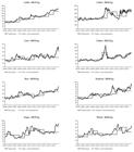
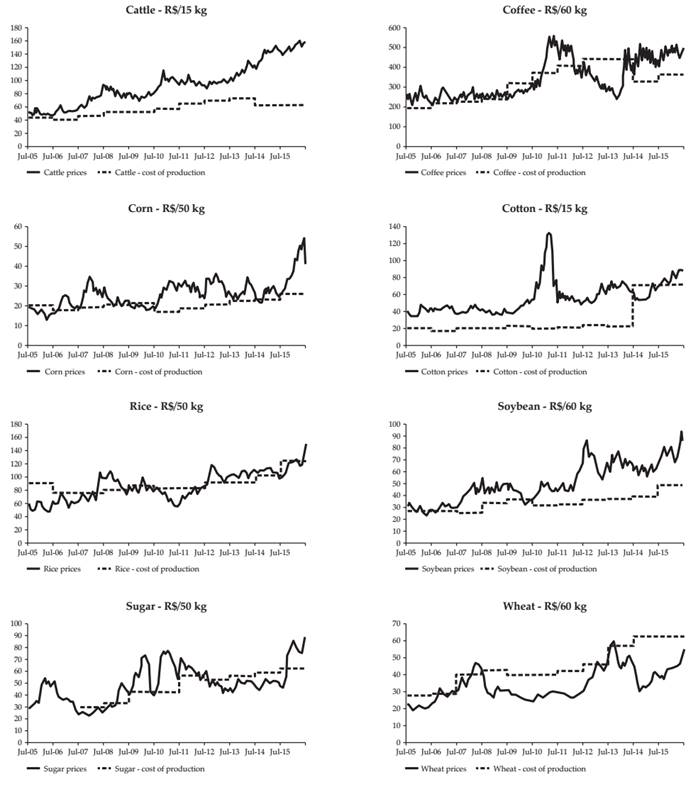
Figures 1 and 2 show daily cash prices for the commodities selected for this study and their respective production costs and minimum prices. These commodities exhibit distinct price behavior over time, not only in terms of how their cash prices moved during the 11 years in our sample but also with respect to their cash prices relative to production costs and minimum prices. For example, cash prices for cattle and soybean were consistently above the average production costs, while cash prices for rice and wheat were often below the average production cost (Figure 1).

Figure 1
Daily cash prices and cost of production, 2005/06 - 2015/16

Figure 2
Daily cash prices and government’s minimum price, 2005/06 - 2015/16

Summary statistics for all commodity price series are presented in Table 1. D’Agostino and Anscombe-Glynn¹² tests were used to test the null hypotheses that skewness equals zero and kurtosis equals 3, respectively. Results show evidence of positive skewness for the price distributions of all commodities but cattle. With respect to kurtosis, results suggest that all price distributions (except cotton) are platykurtic. Therefore, there is evidence that all price distributions are not normally distributed, with commodities exhibiting positive skewness and slim tails, with the exception of cotton, that exhibits positive skewness and fat tail (Table 2).

Table 2
Summary statistics for commodities daily prices, 2005/06 - 2015/16

	Mean	Std. dev.	Median	Max.	Min.	Skewnessa	Kurtosisb
Cattle	93.50	30.71	92.77	159.49	47.14	0.42	-0.66
Coffee	340.34	95.32	292.88	555.19	210.92	0.54	-1.23
Corn	25.93	6.95	25.49	53.91	13.32	1.19	2.53
Cotton	56.29	18.37	52.72	131.95	34.16	1.51	3.05
Rice	29.06	7.05	28.04	50.03	16.12	0.10	-0.97
Soybean	51.05	16.03	47.39	93.18	24.34	0.29	-0.89
Sugar	49.03	15.00	49.21	88.13	23.04	0.30	-0.43
Wheat	33.84	9.10	30.76	59.43	19.06	0.62	-0.46

• (a) D’Agostino test was used to test the null hypothesis that skewness equals zero. The null hypothesis could not be rejected for all series. (b) Anscombe-Glynn test was used to test the null hypothesis that kurtosis equals 3. The null hypothesis could not be rejected for all series.Spurce - Research data.

We use percentage deviations from the benchmark in the calculation of VaR and CVaR. For example, when the benchmark is the cost of production, the daily variables used in the calculation of the risk measures are percentage deviations from the cost of production (e.g. 1.1 would mean that the price was 10% above the cost of production). Summary statistics of these variables are expressed in Table 3. They indicate positive skewness for cattle, corn, cotton, soybean, sugar and wheat, and negative skewness for coffee and rice. All price returns distributions, but cotton, seem to be platykurtic. Normality tests suggest distributions are normally distributed¹³, although four commodities indicate positive skewness and slim tails (cattle, corn, soybean and wheat), three negative skewness and slim tails (coffee, rice and sugar), and one positive skewness and fat tail (cotton).

Table 3
Summary statistics for daily percentage deviations of cash prices from cost of production between 2005/06 and 2015/16^a,b

	Mean	Std. dev.	Median	1st Quartile	3rd Quartile	Max.	Min.	Skewnessc	Kurtosisd
Cattle	1.63	0.37	1.52	1.41	1.74	2.55	1.07	0.99	0.08
Coffee	1.08	0.23	1.11	0.90	1.27	1.56	0.55	-0.37	-0.69
Corn	1.26	0.30	1.20	1.01	1.50	2.06	0.66	0.41	-0.74
Cotton	2.26	1.02	2.16	1.80	2.65	6.71	0.76	1.66	5.04
Rice	0.96	0.18	0.97	0.85	1.09	1.38	0.53	-0.30	-0.20
Soybean	1.46	0.31	1.46	1.21	1.65	2.36	0.89	0.24	-0.38
Sugar	1.08	0.28	0.96	0.87	0.89	1.85	0.75	1.11	0.32
Wheat	0.77	0.15	0.74	0.68	0.86	1.17	0.49	0.66	-0.21

• (a) A rate of return of 10% (-10%) indicates the daily price was 10% above (below) the cost of production. (b) Anderson-Darling and Jarque-Bera test point out to normality in all return series. (c) D’Agostino test was used to test the null hypothesis that skewness equals zero. The null hypothesis could not be rejected for all series. (d) Anscombe-Glynn test was used to test the null hypothesis that kurtosis equals 3. The null hypothesis could not be rejected for all series. Source - Research data.

6. Results

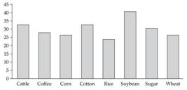
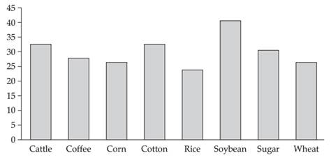
Price risk is first discussed across commodities using the coefficient of variation, i.e. standard deviation divided by the mean. Since all data series are in their original basis, standard deviation tends to be higher (lower) for commodities whose prices are higher (lower). The coefficient of variation offers a more meaningful comparison of price variability across commodities. Values for the coefficient of variation presented in Figure 3 indicate that soybeans present more price variability, followed by cattle, cotton and sugar prices. On the other hand, rice exhibit less price variability. It is important to note that the coefficient of variation suggests that all commodity prices (except for soybeans and rice) appeared to have had similar degrees of variability between 2005/06 and 2015/16.¹⁴

Figure 3
Coefficient of variation for cash prices, 2005/06 - 2015/16 (%)

In order to focus on downside deviations three other risk measures are calculated: LPM, VaR and CVaR. For all of them only deviations below a certain benchmark will be considered. Two benchmarks are adopted: cost of production and government’s minimum price. Note that the government’s minimum price is used here as a reference to discuss how much risk can be avoided by this policy, thus one benchmark is actually the range between cost of production and government minimum price. Since the minimum price is guaranteed by the government, deviations below the cost of production should only be considered risk if they are above the minimum price.

Starting with the lower partial moment of order two (LPM₂), Table 4 presents results for price variability below the two benchmarks. Calculations of lower partial moments suggest that discussions of price variability for each commodity can change depending on whether the focus is on deviations above and below the mean price (e.g. standard deviation and coefficient of variation) or only deviations below a certain benchmark (e.g. LPM). For example, soybeans and cattle exhibited the largest price variability based on the coefficient of variation (Figure 3), but show almost no price variability below their production costs (Table 4). This fact indicates that most variability in soybean and cattle prices occurred above their production costs. Another example is corn, whose coefficient of variation was very similar to all other commodities (except soybean and rice) but whose LPM with respect to production cost is small. Even though corn prices were as volatile as all other commodity prices (except cotton and sugar), most of this variability also occurred above the production cost.

Table 4
Lower Partial Moments (LPM) for different benchmarks, 2005/06 - 2015/16

	Price variability below:
	Cost of production	Cost of production above minimum pricea
Cattle	0.00%	-b
Coffee	54.59%	48.78%
Corn	1.26%	1.20%
Cotton	4.10%	3.90%
Rice	4.53%	3.59%
Soybean	0.50%	0.50%
Sugar	5.32%	-b
Wheat	13.15%	12.90%

• (a) Minimum prices were often set below production costs by the government. (b) There are no minimum price programs for cattle and sugar. Source - Research data.

Note that minimum price programs generally had little impact on the calculation of LPM, since the LPMs across the two benchmarks in Table 3 are very similar (except for cattle and sugar, for which there were no minimum price programs). Soybean prices were consistently above their minimum prices, while corn, cotton and wheat were above their minimum prices during most of the sample period (Figure 2). However, rice and (especially) coffee were the only commodities whose cash prices dropped below the minimum price more frequently, which is why their LPMs show a reduction of 0.94 and 5.81 percentage points, respectively, when measured between the production cost and minimum price rather than only below production cost (Table 4).

Findings from LPM calculations indicate different levels of price variability below production costs, suggesting distinct patterns of potential losses below this benchmark. This point can be further explored with the VaR and CVaR, which will show how much producers can lose if prices fall below the benchmark, i.e. production cost. In this study, VaR and CVaR are based on 95% probability and calculated for each commodity as percentage deviations of daily cash prices from production costs. For example, cotton had a VaR of 21.5%, meaning that its cash price was either above or no more than 21.5% below its production cost in 95% of the days in 2005/06-2015/16. Its CVaR of 23.4% indicates that, in the days when its cash price dropped below the VaR threshold (i.e. more than 21.5% below production cost), the average deviation below production cost was 23.4%.

Summary statistics of the percentage deviations of cash prices with respect to benchmarks show that their distributions exhibit positive means and positive skewness (except coffee and rice). With respect to the tails of the distributions, no variable shows evidence of kurtosis different than 3. Cotton percentage deviations exhibit fat tails (leptokurtic distributions). The other series exhibit slim tails (platykurtic distributions) (Table 2).

Results of VaR and CVaR are presented in Figures 4 and 5, respectively. Point estimates based on historical distributions are shown by the dots inside the charts, while 95% confidence intervals based on nonparametric bootstrap with ordinary simulation and 1,000 replicates are given by the vertical lines crossing each dot (Figures 4 and 5)¹⁵. Results show that both VaR and CVaR are zero for cattle, reflecting the fact that their cash prices have been consistently above their production costs during the sample period (Figure 1). Soybeans indicate small values for VaR and CVaR, as well, reflecting the low variability of its prices below the benchmark (Table 4). Coffee, corn, cotton and sugar exhibit similar values for VaR, indicating potential losses around 21-27%. However, coffee and corn point to larger CVaR values (around 36-37%) than cotton and sugar (close to 23%). The largest values for VaR and CVaR are found for wheat (45.8% and 52.6%, respectively), followed by rice (33.2% and 40.7%, respectively). Additionally, as indicated in Figures 4 and 5, VaR and CVaR confidence intervals point to greater risk dispersion over cotton prices. For example, VaR value for cotton is smaller than corn and sugar. However, if considered the confidence interval limit, cotton downside risk could be higher than corn and sugar.

Figure 4
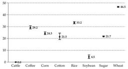
Point estimates and confidence intervals for VaR (in %) using cost of production as the benchmarka,b

Figure 5
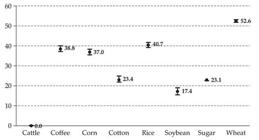
Point estimates and confidence intervals for CVaR (in %) using cost of production as the benchmarka,b

This exercise was also performed for the other benchmark, i.e. below cost of production but above the minimum price determined by the government. In this case, results for alternative VaR and CVaR (including the new benchmark) have not shown significant changes for all commodities, with the exception of rice, that exhibited significant decrease in price risk (Figures 6 and 7, Appendix). This is consistent with the fact that rice was one of the commodities whose cash prices were often below the minimum price during the sample period (Figure 2). Considering deviations below the production cost but above the minimum price, VaR and CVaR values for rice are 27.2% and 33.5%, respectively, which are smaller than values found for wheat and similar to the ones found for corn. Although the VaR and CVaR reduction for coffee and wheat under the new benchmark, the values exhibit slight variation from the original benchmark. VaR and CVaR values for coffee are 27.3% and 37%, and for wheat 45.8% and 51.8%. Therefore, we can observe that rice decreases its downside risk to similar level than coffee, isolating wheat as the highest price risk below cost of production benchmark.

We have discussed findings related to LPM, VaR and CVaR using two benchmarks: production cost and production cost above the minimum price set by the government. Those two were chosen because production costs are a natural benchmark for farmers, since they often see their cost of production as their break-even point. Minimum prices were also chosen because farmers do not think about risk or potential losses below those levels, since they are guaranteed by the government. However, other benchmarks could also be considered, such as historical prices or prices reflecting farmers’ aspirations (KAHNEMAN and TVERSKY, 1979; BAUCELLS et al., 2011). Thus we also conducted the same analysis using a third reference price, which is the previous year’s average cash price (Figure 8, Appendix). Results were qualitatively the same as what has already been discussed and will not be presented for brevity, but are available upon request.

One last issue needs to be addressed regarding the cash prices used in this study. Except for cattle and sugar, whose cash prices represent prices received by producers at the farm gate, the other cash prices include freight since they reflect prices paid at the delivery location. Therefore, for coffee, corn, cotton, rice, soybeans and wheat, prices actually received by producers should be lower (by the amount of the freight) than those used in this study. Therefore, individual results for LPM, VaR and CVaR should be larger than presented here.

Data on freight costs were not included in the analysis because they are not readily available. Only qualitative information was obtained, which provided some useful insights. The distances between delivery locations and producing areas adopted in this study were typically around 15-50 miles, indicating that freight rates would generally be small. In addition, prices of fuel, one of the major components of freight costs, were controlled by the federal government during most of the sample period and showed little changes. Finally, simple qualitative analysis of prices and benchmarks suggests that freight costs might not make much difference in the results for some commodities. For example, cattle, cotton (until 2014) and soybeans (from 2010) prices including freight were about twice as high as the cost of production, and even higher compared to the government’s minimum price. Thus, these prices would likely continue being above the two benchmarks even if freight was discounted, and thus its LPM, VaR and CVaR would still be small.

Lastly, regardless the impact of the inclusion of freight costs in the prices of most commodities discussed in this study, it can be argued that the basic idea of the paper would still be valid. That is, different ways to measure risk can generate distinct insights to the discussion of price risk in commodity markets.

7. Conclusion

The purpose of this study was to explore price risk in commodity markets through alternative measures. In particular, this research focused on downside risk and investigated how risk assessment across commodities can change with one-sided measures vis-à-vis two-sided measures. Results from this study suggest that the question of which commodity exhibits more price risk can have different answers depending on how risk is perceived. If risk is measured by the coefficient of variation (standard deviation), soybeans emerge as the riskiest markets in Brazil between 2005 and 2016, while all other commodities would have relatively lower levels of risk. On the other hand, if risk is measured by VaR and CVaR, wheat, rice and coffee would be highlighted as the riskiest markets, while cattle and soybeans would be among the least risky commodities.

These findings emphasize two related issues that have been discussed in the marketing and risk management literatures. First, there is not a single definition of risk. In a marketing context, different producers can think of risk in different ways, e.g. some producers can be concerned about any price variability while others might think of risk only as the failure to achieve a certain benchmark. Individuals who think about risk in terms of price volatility, or variability in their revenues, would focus more on the standard deviation and coefficient of variation. In that case, they would rank soybeans, cattle, cotton and sugar as the riskiest markets in Brazil between 2005 and 2016. On the other hand, individuals who perceive risk as the magnitude of potential losses would indicate rice and wheat as the riskiest commodities in Brazil in 2005-2016, leaving cattle and soybeans among the least risky ones. Second, producers who are mainly focused on downside risk, the choice of a benchmark can have large implications on the amount of risk they face. In this current research, discussion about downside risk was concentrated on cost of production and government’s minimum price as benchmarks, but the average price of the previous crop-year was also considered as a possible benchmark with similar qualitatively results.

Our findings can have implications for many agents in the agricultural industry. In general, our results can help clarify the discussion about risk measurement and risk perception. Our outcomes show that risk levels across commodities can differ depending on how they are measured. This raises the importance of determining whether risk will be defined as price variability or only downside deviations, and then whether this variability and deviations should be taken from the mean of the price series or another benchmark. These two points are crucial in the calculation of risk and can generate very different results. For example, producers who grow commodities with high price variability are exposed to more uncertainty in revenues but not necessarily to more losses. On the other hand, producers who grow commodities with large VaR and CVaR are more exposed to losses but not necessarily to more uncertainty in revenues. This distinction is important for all agents dealing with commodity marketing, such as producers, marketing advisors who work with producers, and risk managers in processing and exporting firms. Having a clear understanding of how they perceive risk and its implications on the calculation of how much risk they face can help them design and implement appropriate risk management strategies.

Further, policy makers can also benefit from a better understanding and communication to the public of distinct types of risk in different commodity markets. Our results generally suggest that wheat has been the commodity with greatest downside risk in Brazil, followed by rice and coffee. This finding is consistent with anecdotal evidence that rice and wheat growers have often complained about low profits, rising debts and absence of market-oriented risk management tools (such as forward and futures contracts). This situation motivated the federal government to allocate subsidized funding for marketing and storage in the rice and wheat sectors, which became increasingly dependent on government support. Apart from the debate on whether government should support farmers or not, our findings indicate that rice and wheat producers have indeed been exposed to more downside risk and potential losses than other producers. The clarification and dissemination of different ways to measure risk can be useful in policy debates about government support to agriculture.

Despite the results of the debate about government intervention in agriculture, there has recently been a general trend of tighter control of federal government budget, which may lead to less funding allocated to agricultural subsidies in Brazil. Similarly, increasing income might reduce concerns about food security, making government less worried about supporting food commodities. This brings a specific example of how our results can be applied to real-world problems. The trends indicated above suggest risk management might become ever more important for commodity producers in general, and maybe more so for rice and wheat producers. The development of risk management instruments and marketing contracts may be essential in an environment with less government intervention. A careful discussion on how risk is perceived and measured should guide the development of appropriate mechanisms to manage risk (e.g. contracts, diversification, and insurance) according to how agents perceive risk.

Another important issue to consider is related to the dynamics of agricultural markets price discovery. Overall, our findings suggest that most of the markets in which Brazil is a major exporter (e.g. soybeans, cattle, sugar), price risk seems to be smaller in comparison to other markets in which Brazilian agents follow the international market (e.g. wheat and rice). Further research can explore these findings in a comprehensive analysis of each market and their price discovery process in association to price risk.

Finally, future research can advance the issues discussed here by empirically investigating how producers and other agents in the agricultural industry actually perceive risk. This could be done with laboratory or field experiments to explore how individuals form their ideas about risk and how those ideas evolve over time. These insights would be useful in the discussion of appropriate risk measures to use for distinct agents, including the determination of possible benchmarks relevant for risk perception.

8. References

• BAWA, V. S. Safety-first, stochastic dominance, and optimal portfolio choice. Journal of Financial and Quantitative Analysis, v. 13, n. 2, p. 255-271, 1978.
• BAUCELLS, M., WEBER, M. and WELFENS, F. Reference-point formation and updating. Management Science, v. 57, n. 3, 506-519, 2011.
• BRAZILIAN AGRICULTURAL CONFEDERATION - CNA. Sugar: cost of production. Brasilia, DF, Brazil, 2016. Available at <http://www.cna.org.br>.
  » http://www.cna.org.br
• BRAZILIAN BEEF EXPORTERS ASSOCIATION - ABIEC. Statistics. Sao Paulo, SP, Brazil, 2017. Available at <http://www.brazilianbeef.org.br/>.
  » http://www.brazilianbeef.org.br/
• BRAZILIAN INSTITUTE OF GEOGRAPHY AND STATISTICS - IBGE. Agricultural and livestock census. Rio de Janeiro, RJ, Brazil, 2016. Available at <http:// www.sidra.ibge.gov.br>.
  » http:// www.sidra.ibge.gov.br
• BRAZILIAN NATIONAL SUPPLY COMPANY - CONAB. Agricultural cost of production. Brasilia, DF, Brazil, 2016. Available at <http://www.conab.gov.br/>.
  » http://www.conab.gov.br/
• BRAZILIAN SUGARCANE INDUSTRY ASSOCIATION - UNICA. Sugarcane harvest reports. São Paulo, SP, Brazil, 2016. Available at <http://www.unicadata.com.br/>.
  » http://www.unicadata.com.br/
• CAMPOS, K. C. Análise da volatilidade de preços de produtos agropecuários no Brasil. Revista de Economia e Agronegócio, v. 5, n. 3, p. 303-328, 2007.
• CENTER FOR ADVANCED STUDIES ON APPLIED ECONOMICS - CEPEA/USP. Prices indexes. Piracicaba, SP, Brazil, 2016. Available at <http://www.cepea.esalq.usp.br/>.
  » http://www.cepea.esalq.usp.br/
• CHEN, S. S., LEE, C. and SHRESTHA, K. Futures hedge ratios: a review. The Quarterly Review of Economics and Finance, v. 43, n. 3, p. 433-465, 2003.
• COELHO, C. N. 70 anos de Política Agrícola no Brasil (1931-2001). Revista de Política Agrícola, ano 10, n. 3, p. 03-58, jul./set. 2001.
• COMTRADE. International trade statistics database: commodity trade statistics. New York, 2016. Available at <http://www.comtrade.un.org>.
  » http://www.comtrade.un.org
• CONT, R. Empirical properties of asset returns: stylized facts and statistical issues. Quantitative Finance, v. 1, n. 1, p. 223-236, 2001.
• FISHBURN, P. C. 1977. Mean-risk analysis with risk associated with below-target returns. The American Economic Review, v. 67, n. 2, p. 116-126.
• FREITAS, C. A. and SÁFADI, T. Volatilidade dos retornos de commodities agropecuárias brasileiras: um teste utilizando o modelo APARCH. Revista de Economia e Sociologia Rural, v. 53, n. 2, p. 211-228, abr./jun. 2015.
• GARCIA, J. R. and VIEIRA FILHO, J. E. Brazilian agricultural policy: productivity, inclusion and sustainability. Revista de Política Agrícola, ano 23, n. 1, p. 91-104, jan./mar. 2014.
• GROOTVELD, H. and HALLERBACH, W. Variance vs downside risk: is there really that much difference? European Journal of Operational Research, v. 114, n. 2, p. 304-319, 1999.
• HARRIS, R. D. F. and SHEN, J. Hedging and value at risk. Journal of Futures Market, v. 26, n. 4, p. 369-390, 2006.
• INFORM ECONOMICS - FNP. Anuelpec online: cattle cost of production data. São Paulo, SP, Brazil, 2016. Availabe at <http://www.informaeconomic-fnp.com/publicacoes>.
  » http://www.informaeconomic-fnp.com/publicacoes
• JORION, P. Value at risk - the new benchmark for managing financial risk. New York: McGrall-Hill, 2001.
• KAHNEMAN, D. and TVERSKY, A. Prospect theory: An analysis of decision under risk. Econometrica, v. 47, n. 2, p. 263, 1979.
• LIANG, B. and PARK, H. Risk measures for hedge funds: a cross-sectional approach. European Financial Management, v. 13, n. 2, p. 333-370, 2007.
• LIEN, D. and TSE, Y. K. Some recent developments in futures hedging. Journal of Economic Surveys, v. 16, n. 3, p. 357-396, 2002.
• MARKOWITZ, H. M. Portfolio selection: efficient diversification of investments. New York, NY: John Wiley & Sons, 1959.
• MOSCHINI, G. and HENNESSY, D. A. Uncertainty, risk aversion, and risk management for agricultural producers. In: GARDNER. B . and RAUSSER G. , (Eds.). Handbook of agricultural economics. North Holland: Elsevier, 2001, p. 87-153.
• PEREIRA, V. F. et al. Conditional volatility of the returns from Brazilian agricultural commodities. Revista de Economia, v. 36, n. 3, 73-94, set./dez. 2010.
• RACHEV, S. T., MENN, C. and FABOZZI, F. J. Risk measures and portfolio selection. In: RACHEV, S. T.; MENN, C.; FABOZZI, F. J. (Eds.). Fat-tailed and skwed asset returns distributions: implications for risk management, portfolio selection, and option pricing. New York, NY: John Wiley & Sons , 2005, p. 181-198.
• ROY, A. D. Safety first and the holding of assets. Econometrica, v. 20, n. 3, p. 431-450, 1952.
• UNSER, M. Lower partial moments as measures of perceived risk: an experimental study. Journal of Economics Psychology, v. 21, n. 1, p. 253-280, 2000.
• VELD, C. and VELD-MERKOULOVA, Y. The risk perceptions of individual investors. Journal of Economic Psychology, v. 29, n. 2, p. 226-252, 2008.

• 4
  . The federal government establishes a minimum price for these commodities and, if market prices are below that level, it buys from producers at the minimum price.

• 5
  . They are, in principle, the same notion initially discussed by Markowitz (1959) and Roy (1952).

• 6
  . Alternatively, there is a 5% probability that this portfolio will lose at least $100,000 over 1 year.

• 7
  . For conditional variance analysis in the Brazilian agricultural market, see Campos (2007); Pereira et al. (2010); Freitas and Sáfadi (2015).

• 8
  . There are four main producing areas for cattle, one for coffee, two for corn, one for cotton, five for rice, four for soybeans, one for sugar and four for wheat.

• 9
  . Except cotton, rice and wheat, which do not have a futures contract in Brazil.

• 10
  . Note that minimum price programs are not available for cattle and sugar producers.

• 11
  . It is important to point out that producers may use alternative tools to mitigate their price risk, such as establishing forward contracts, operating in the futures/option markets, as well as making decisions over storage and trade.

• 12
  . D’Agostino test computes the skewness and kurtosis to quantify how far the distribution is from Gaussian (normality) in terms of asymmetry and shape. It assumes in the null hypothesis that data has asymmetry equal to zero (skewness equal to 0). Anscombe-Glynn test for kurtosis is a powerful tool to detect normality due to nonnormal kurtosis. In this test, under the hypothesis of normality, data should have skewness equal to 3, instead of different from 3 in the alternative hypothesis.

• 13
  . Derived from D’Agostino test for skewness, Anscombe-Glynn test for kurtosis, Anderson-Darling and Jarque-Bera tests for normality.

• 14
  . Results for commodities whose data referred to more than one production region are presented as a simple average of all regions for brevity. There is little variability in results across regions for the same commodity. Individual results for each production region may be provided upon request.

• 15
  . Bootstrap simulations with one thousand replications for each variable were used to determine the VaR and CVaR confidence interval.

Appendix

Figure 6
Point estimates and confidence intervals for VaR (in %) using cost of production as the benchmark and considering government’s minimum pricea

Figure 7
Point estimates and confidence intervals for CVaR (in %) using cost of production as the benchmark and considering government’s minimum pricea

Figure 8
Daily cash prices and previous year’s average price, 2005/06 - 2015/16

Publication Dates

• Publication in this collection
  Jul-Sep 2017

History

• Received
  18 Aug 2016
• Accepted
  21 May 2017