Exploring the key analogies and differences in Bernoulli’s equations for incompressible and compressible flow

Abstract

This study explores key analogies and differences between the conventional Bernoulli’s Equation for Incompressible Flow (BEIF) and its compressible counterpart (BECF) for ideal gases, excluding gravitational effects. Comparing both equations, we identify terms for kinetic energy, thermal energy, and pressure. A crucial distinction is that the thermal energy per unit mass is spatially uniform and implicit in BEIF, whereas in BECF it is spatially variable and explicit. We demonstrate that BECF reduces to BEIF when the molecular number of degrees of freedom is zero, equivalent to replacing the non-uniform thermal energy of a gas with the uniform one of an incompressible fluid. We generalize the BEIF interpretations of energy or enthalpy conservation per unit mass to BECF. Furthermore, we develop a microscopic interpretation for BECF incorporating an isotropic squared-speed particle distribution and intermolecular interactions. Counterintuitively, the analogous BEIF interpretation implies that microscopic kinetic energy cannot convert into macroscopic forms in incompressible flows. Finally, analysis of the velocity-pressure-density relationship using dimensionless equations reveals that BECF’s convergence to BEIF involves a complex coupling among these variables. While both equations predict maximum flow velocities at zero pressure, incompressible fluids can reach it, whereas compressible fluids cannot, as pressure and density approach zero simultaneously.

Keywords:
Bernoulli’s equation; Compressible flow; Physical interpretation; Enthalpy; Particle level.

1. Introduction

Undergraduate students learn that Bernoulli’s equation is fundamentally derived for incompressible, inviscid, and steady flows [¹, ², ³, ⁴]. Furthermore, while this standard formulation is strictly valid only under these conditions, textbooks often extend it to compressible flows at low Mach numbers¹ (typically below $M=0.7$), where velocity variations remain below approximately 6%, thus exhibiting nearly incompressible behavior [⁴]. To describe compressible flows outside this low-Mach regime, a dedicated Bernoulli’s equation for compressible fluids is required [⁴]. Although the physical meaning of the incompressible Bernoulli’s equation is deeply explored in the literature [⁵, ⁶, ⁷, ⁸, ⁹, ¹⁰, ¹¹], a corresponding analysis for the compressible flow equation remains scarce.

In this work, the term inviscid fluid refers to a fluid with zero viscosity, such that internal friction forces are neglected. A flow is deemed incompressible when density variations are negligible throughout the motion, whereas in a compressible flow such density changes cannot be ignored. In practice, all real fluids are viscous and, strictly speaking, compressible; however, Bernoulli’s equation can be applied to liquids and low-speed gas flows in regions where viscous effects are small [¹, ², ³, ⁴].

We adopt in this work the following terminology to distinguish the two versions of Bernoulli’s equation: Bernoulli’s equation for incompressible flow (BEIF) and Bernoulli’s equation for compressible flow (BECF).

Usually, BEIF is presented as [¹, ², ³]

(1) $$\frac{\rho U^2}{2}+\rho gh+P=P_0,$$

where $\rho$, $U$, $g$, $h$, $P$, $P_0$ are fluid density, flow velocity, gravitational acceleration, height, pressure, and stagnation pressure, respectively. The stagnation pressure, $P_0$, is the pressure for $U=0$ and $h=0$. Each streamline is associated with a specific value of stagnation pressure, $P_0$. In the teaching about BEIF, the terms $\rho U^2/2$, $\rho gh$ and $P$ are named “dynamic pressure”, “hydrostatic pressure” and “static pressure”, respectively [²]. In the terminilogy of this work, we designate static pressure simply as “pressure”.

An example of BEIF application is water distribution in building pipes. When pipe diameter decreases, velocity $U$ increases and pressure $P$ decreases (equation 1). Additionally, the first floor has minimum height $h$, yielding maximum hydrostatic pressure $P$ (equation 1).

The dynamic pressure ($\rho U^2/2$) and hydrostatic pressure ($\rho gh$) represent kinetic and gravitational potential energy densities, respectively. The role of pressure can be understood through the pressure gradient force density, $\overrightarrow{f}=-\nabla P$[⁹]. When pressure decreases along a streamline, the force density $\overrightarrow{f}=-\nabla P$ accelerates fluid elements, increasing their kinetic energy. Conversely, increased pressure leads to flow deceleration and a reduction in kinetic energy reduction [⁹].

In general, pressure itself is not an energy density [⁵, ⁸, ⁹]. Consequently, some authors argue that pressure should not be interpreted as an energy density, and instead view BEIF as representing conservation of enthalpy density along streamlines [⁸, ⁹, ¹²]. In this interpretation, the stagnation pressure $P_0$ corresponds to the enthalpy density. This perspective is referred to as the “enthalpy interpretation” [⁹].

Specifically for stationary flows, pressure behaves as a type of potential energy density [⁹]. Building on this concept, other authors argue that pressure effectively represents a form of potential energy density, contrasting with the enthalpy interpretation [⁶, ⁷, ⁹]. In this view, BEIF expresses conservation of mechanical energy density along each streamline [⁹], with the stagnation pressure $P_0$ corresponding to the total mechanical energy density. This interpretation is called the “energy interpretation” [⁹].

A third interpretation posits that BEIF expresses the balance between ordered macroscopic kinetic energy ($\rho U^2/2$) and disordered microscopic kinetic energy [⁸, ¹⁰, ¹¹, ¹³]. Within this framework, BEIF represents the conservation of energy density along each streamline, stagnation pressure $P_0$ corresponds to the total energy density, while, in contrast to the energy interpretation, pressure is interpreted as a fraction of the kinetic energy density associated with the random motion of fluid particles at the microscopic level [⁸, ¹⁰, ¹¹, ¹³]. Notably, some authors have successfully derived BEIF without the gravitational term, $\rho gh$, directly from a model based on this interpretation [¹¹, ¹³]. We designate this as the “conventional microscopic interpretation”.

Some authors criticize two problematic premises of the conventional microscopic interpretation model: (1) the statistical distribution of particle squared speeds in random motion would be anisotropic [⁸, ¹¹, ¹³], contradicting established principles of fluid kinetic theory [¹², ¹⁴]; and (2) interactions between particles would be limited to perfectly elastic mechanical collisions [⁸, ¹¹, ¹²], which describes ideal gases [¹⁵] but not incompressible fluids [¹⁶]. The BEIF derived under this approach constitutes a valid conclusion drawn from false premises [¹²]. Using an isotropic distribution of particle squared speeds and more general interparticle interactions, a rigorous kinetic theory predicts the Navier-Stokes equations, which generalize BEIF through the inclusion of viscous and time-dependent effects [¹⁴].”

The BECF is presented as [⁴]

(2) $$\frac{U^2}{2}+\left(\frac{\gamma }{\gamma -1}\right)\frac{P}{\rho }=\left(\frac{\gamma }{\gamma -1}\right)\frac{P_0}{{\rho }_0},$$

where $\gamma$ and ${\rho }_0$ denote the adiabatic index and stagnation fluid density, respectively. The stagnation fluid density, ${\rho }_0$, is the fluid density if $U=0$ and $P=P_0$. Each streamline has specific $P_0$ and ${\rho }_0$. In this work, we apply BECF only to ideal gases² composed of identical molecules to facilitate exploration through kinetic theory of gases [¹⁵]. Ideal gases without heat transfer obey the adiabatic condition,

(3) $$\frac{P}{{\rho }^{\gamma }}=\frac{P_0}{{\rho }_0^{\gamma }}.$$

The literature contains two versions of BECF: one including gravitational effects [¹²] and another without them [⁴]. In this work, we use the non-gravitational version 2.

An example of BECF without gravitational effects is wind dynamics. Between two regions, the air moves from the high-pressure zone to the low-pressure zone, and its speed increases toward the low-pressure side.

This work provides a comparative analysis of BEIF and BECF. The analysis begins by rewriting both equations in analogous terms without gravitational effects, an approach that immediately reveals a fundamental contrast: the very process of aligning their analogous terms most clearly illuminates their key physical differences. Subsequently, we generalize energy and enthalpy interpretations from BEIF to BECF and, conversely, formulate a new microscopic interpretation for BECF that is also applied to BEIF. The study completes the comparison between BEIF and BECF by analyzing how the different density behaviors of incompressible and compressible fluids impact both equations across low and high velocities. This analysis is performed by rewriting both equations in terms of dimensionless parameters.

Section 2 presents a direct comparison between BEIF and BECF. Section 3 then establishes BEIF as a degenerate particular case of BECF. Building on this framework, Sections 4 and 5 extend the energy and enthalpy interpretations from BEIF to BECF, respectively. Section 6 analyzes BECF using results from the kinetic theory of gases to develop an isotropic interpretation, which is subsequently adapted for BEIF. Section 7 incorporates fluid density behavior into the BEIF-BECF comparison, exploring the relationship among velocity, pressure, and fluid density, across both low and high velocity regimes. The paper concludes with a general discussion (Section 8) and final conclusions (Section 9).

2. Comparison Between the Two Equations

To compare BEIF and BECF, we first rewrite BEIF (equation 1) in terms of energy per unit mass and without gravitational effects as

(4) $$\frac{U^2}{2}+\frac{P}{\rho }=\frac{P_0}{\rho }.$$

The term $U^2/2$ represents the kinetic energy per unit mass. This is evident when considering a fluid element of mass $\delta m$ and velocity $U$: its kinetic energy, $\delta m{U}^2/2$, divided by its mass $\delta m$, yields $U^2/2$. The term $P/\rho$ originates from the work done by pressure forces, which is derived from the pressure gradient, $\overrightarrow{f}=-\nabla P$. We designate $U^2/2$ and $P/\rho$ as kinetic and pressure terms, respectively.

We rewrite BECF equation 2 as

(5) $$\frac{U^2}{2}+\frac{P}{\rho }+\frac{n_{f}P}{2\rho }=\frac{P_0}{{\rho }_0}+\frac{n_f{P}_0}{2{\rho }_0},$$

where the adiabatic index, $\gamma$, is related to the number of molecular degrees of freedom available for energy storage, $n_f$, by

(6) $$\gamma =\frac{n_f+2}{n_f}.$$

The relationship between $\gamma$ and $n_f$ is a key prediction of the kinetic theory of gases [¹⁵]. For monatomic ideal gases, $n_f=3$, corresponding exclusively to translational kinetic energy. Polyatomic molecules possess additional degrees of freedom ($n_f>3$) arising from rotational and vibrational modes.

The terms $U^2/2$ and $P/\rho$ appear in both BEIF (equation 4) and BECF (equation 5); thus they must have the same interpretation in both equations. However, the term $n_{f}P/2\rho$ in equation 5, which is present only in BECF, represents the thermal energy per unit mass for ideal gases. The term $n_f{P}_0/2{\rho }_0$ in BECF (equation 5) represents the thermal energy per unit mass when $U=0$; we refer to $n_{f}P/2\rho$ and $n_f{P}_0/2{\rho }_0$ as the thermal and stagnation thermal terms, respectively.

The proof that $n_{f}P/2\rho$ represents the thermal energy per unit mass is presented as follows: in the kinetic theory of gases, if the squared speed distribution of $N$ identical molecules is isotropic, the thermal energy of a portion of ideal gas at rest, $E_{th0}$, with temperature $T_0$, pressure $P_0$, volume $V_0$, and without gravitational effects is given by

(7) $$E_{th0}=\frac{n_{f}N{k}_B{T}_0}{2}=\frac{n_f{P}_0{V}_0}{2},$$

where $k_B$ is the Boltzmann constant. Considering fluid density $\rho =m/V$, according to equation 7, the thermal energy per unit mass, ${\epsilon }_{th0}$, is

(8) $${\epsilon }_{th0}=\frac{E_{th0}}{m}=\frac{n_f{P}_0}{2{\rho }_0}.$$

When the gas moves with velocity $U$, the speed of each particle is $U$ plus a random speed component with an isotropic distribution of squared speed. Each speed component is related to a form of energy. The component $U$ is associated to the kinetic term, $U^2/2$, in BECF (equation 5). The particle random speed is associated with the microscopic kinetic energy. The sum of this microscopic kinetic energy with the molecular energies from rotations and vibrations is precisely the thermal energy for the gas in motion, $n_{f}P/2\rho$, as we set out to prove. We omitted the index 0 from expression 8 in $n_{f}P/2\rho$ because the gas is in motion.

A term involving the thermal energy does not appear in the BEIF (equations 1 and 4). Unlike ideal gases, pressure and temperature are independent in incompressible fluids. The thermal energy in incompressible fluids depends only on temperature, not on pressure. Heat transfer in incompressible fluids is proportional to temperature variation, $Q=C\Delta T$. Thus, pressure variations in BEIF do not change the temperature nor the thermal energy per unit mass.

Without external heat sources and with no viscous dissipation in inviscid incompressible fluids, there is no heat transfer ($Q=0$), and temperature remains constant ($\Delta T=0$). A uniform and constant temperature implies that thermal energy per unit mass is also constant and uniform in inviscid incompressible fluids. We can therefore add the uniform and constant thermal energy per unit mass ${\epsilon }_{th}$ to equation 4,

(9) $$\frac{U^2}{2}+\frac{P}{\rho }+{\epsilon }_{th}=\frac{P_0}{\rho }+{\epsilon }_{th}.$$

Thus, the only difference between BEIF (equation 9) and BECF (equation 5) is the thermal term: the uniform ${\epsilon }_{th}$, and non-uniform $n_{f}P/2\rho$.

3. Unifying the Two Equations

Although mathematically $n_f=0$ is possible in equation 5, ideal gases can store energy in at least the three spatial directions ($n_f\ge 3$). However, BEIF in equation 4 is a particular case of BECF in equation 5, provided that we admit the possibility $n_f=0$. Analogously to approaching a circumference as a degenerate ellipse with zero focal distance, BEIF behaves as a degenerate BECF with $n_f=0$.

As the ideal gases, the molecules of the incompressible fluids present translational motion, rotations and vibrations. Thus, $n_f=0$ in BECF (equation 5) does not mean that an ideal gas can have zero degrees of freedom. In incompressible fluids, any energy variations at the molecular level are immediately rebalanced by intermolecular interactions, keeping the temperature and density constant, and the thermal energy does not depend on pressure. Unlike the thermal term $n_{f}P/2$ in BECF for compressible fluids (equation 5), we can neglect the uniform and constant thermal term ${\epsilon }_{th}$ in BEIF (see equations 4 and 9). The condition $n_f=0$ is a mathematical artifice for neglecting the thermal term ($n_{f}P/2=0$) in BECF (equation 5) for reducing to BEIF (equation 4). In the specific case $n_f=0$, $n_f$ does not represent the number of degrees of freedom.

Although the uniform and constant thermal term ${\epsilon }_{th}$ in BEIF (equation 9) can be neglected, it is necessary for comparing BEIF and BECF, and in the physical interpretation of BEIF at the particle level.

While equation 5 elegantly unifies both equations, it also highlights a fundamental distinction between them: the behavior of the fluid density. The BEIF describes a flow with a uniform fluid density, $\rho ={\rho }_0$. In contrast, BECF obeys the adiabatic relation (equation 3), showing a critical dependence of fluid density on pressure and velocity. This profound difference in how fluid density is treated underpins the distinct physical behavior predicted by the BEIF and BECF.

4. Energy Interpretation

When applying the energy interpretation in equation 1, the pressure arises as a type of potential energy density, thus there is a “pressure potential energy”. In a fluid element of volume $\delta V$, the potential pressure energy for a gas with pressure $P$ is $P\delta V$. The potential pressure energy per unit mass in a fluid element of mass $\delta m$ is given by

(10) $$\frac{P\delta V}{\delta m}=\frac{P}{\rho },$$

where fluid density is $\rho =\delta m/\delta V$.

Thus, in the energy interpretation, the term $P/\rho$ in BECF (equation 5) represents the potential pressure energy per unit mass (equation 10). Consequently, according to this interpretation, BECF implies that the sum of the kinetic, pressure, and thermal terms remains constant along each streamline (see equation 5). The constant $P_0/{\rho }_0+n_f{P}_0/2{\rho }_0$ is the total energy per unit mass in each streamline.

Within the energy interpretation of BECF, the constancy and uniformity of energy per unit mass along a streamline underscore that this energy is carried with the fluid as it moves. Consequently, this framework does not account for the flow of thermal energy independent of matter, as occurs in mechanisms such as heat conduction between stationary solid bodies.

The energy interpretation for the BEIF becomes a particular case of the same physical view for BECF (equation 5). However, a peculiarity of the BEIF in the energy interpretation lies in the coupling between thermal and mechanical energy. In general, in equation 5, the thermal term, $n_{f}P/2\rho$, is dynamically linked to the mechanical energy terms, $U^2/2+P/\rho$, through the pressure. However, when $n_f=0$, the thermal term vanishes ($n_{f}P/2\rho =0$), and only the mechanical energy terms ($U^2/2+P/\rho$) remain constant. For the BEIF (equation 9), the thermal term, ${\epsilon }_{th}$, is uniform and decoupled from the mechanical energy balance defined by equation 4. Thus, the BEIF represents the conservation of mechanical energy alone, independent of thermal effects, and constitutes only one aspect of the broader energy conservation framework.

5. Enthalpy Interpretation

According to the enthalpy interpretation of BEIF in equation 1, pressure is not a type of potential energy. Consequently, “potential pressure energy” does not exist, and the quantity $P\delta V$ in equation 10 cannot be interpreted as an energy. It follows that the term $P/\rho$ must not represent an energy per unit mass.

The enthalpy $H$ of a fluid with total energy $E$, pressure $P$, and volume $V$ is defined as $H=E+PV$. For a fluid element of mass $\delta m$, and volume $\delta V$, with total energy $\delta E$, its enthalpy is $\delta H=\delta E+P\delta V$. The enthalpy per unit mass $h_m$ is therefore given by

(11) $$h_m=\frac{\delta H}{\delta V}=\frac{\delta E+P\delta V}{\delta m}=\epsilon +\frac{P}{\rho },$$

where $\epsilon =\delta E/\delta m$ represents the total energy per unit mass.

If we adopt the enthalpy interpretation for BECF (equation 5), identify the sum $P_0/{\rho }_0+n_f{P}_0/2{\rho }_0$ as the enthalpy per unit mass, $h_m$, and compare equations 5 and 11, we obtain the total energy per unit mass,

(12) $$\epsilon =\frac{U^2}{2}+\frac{n_{f}P}{2}.$$

We generalize the enthalpy interpretation from BEIF to BECF. The enthalpy interpretation for the BEIF in equation 1 implies that the energy density is not uniform [⁹]. This non-uniformity does not violate energy conservation, as pressure variations perform work on the fluid, thereby changing its energy [⁹]. Extending this principle to BECF, the total energy per unit mass in the enthalpy interpretation (equation 12), when analyzed via BECF (equation 5), also varies along each streamline. The work per unit mass associated with the $P/\rho$ term is the mechanism that alters this total energy.

6. Isotropic Microscopic Interpretation

The conventional microscopic interpretation fails for BECF because the expression of the thermal energy per unit mass, $n_{f}P/2\rho$, is explicitly based on the isotropic distribution of the random squared speed (see Section 2). For this reason, we develop a new microscopic interpretation for BECF by leveraging the more tractable framework of the kinetic theory of gases.

According to equation 8 from the kinetic theory of gases, for a monoatomic ideal gas at rest ($n_f=3$), the thermal term, $3P/2\rho$, consists solely of the microscopic translational kinetic energy. For polyatomic molecules ($n_f>3$), the thermal term, $n_{f}P/2\rho$, can be partitioned into the translational kinetic energy per unit mass, ${\epsilon }_{trans}=3P/2\rho$, and the molecular energy per unit mass associated with rotational and vibrational modes, ${\epsilon }_{int}=\left(n_f-3\right)P/2\rho$. Therefore, the microscopic kinetic energy constitutes only a part of the total thermal energy in a polyatomic gas.

In BECF (equation 5), the thermal term is $n_{f}P/2\rho$, which includes the microscopic kinetic energy, ${\epsilon }_{trans}=3P/2\rho$. Since this thermal energy can be converted into other forms, it follows that microscopic and macroscopic kinetic energy per unit mass can transform into each other.

In the conventional microscopic interpretation for BEIF, pressure $P$ is viewed as a fraction of the microscopic kinetic energy density. This implies that the term $P/\rho$ represents a form of microscopic kinetic energy per unit mass. However, BECF (equation 5) presents the pressure term $P/\rho$ and the thermal term $n_{f}P/2\rho$ as distinct quantities. In an alternative microscopic interpretation, while the interconversion between microscopic and macroscopic kinetic energy must be retained, the direct identification of $P/\rho$ itself as microscopic kinetic energy is excluded.

Based on our preliminary results, we propose an “isotropic microscopic interpretation” for the BECF in equation 5, which describes the balance along a streamline between three distinct quantities: the thermal energy in $n_{f}P/2\rho$ (which includes the microscopic kinetic energy in $3P/2\rho$); the macroscopic kinetic energy in $U^2/2$; and the work associated with the pressure gradient in $P/\rho$.

The isotropic microscopic interpretation reveals contrasts between $P/\rho$ and $n_{f}P/2\rho$: the first term is macroscopic while the second, microscopic; moreover, $P/\rho$ depends on pressure gradients, whereas $n_{f}P/2\rho$ is a local quantity.

Furthermore, the isotropic microscopic interpretation is compatible with the macroscopic enthalpy and energy interpretations, offering two complementary perspectives. If $P/\rho$ is not considered an energy density per unit mass, the result is the classical conservation of enthalpy. Conversely, if $P/\rho$ is interpreted as a pressure potential energy per unit mass, it becomes part of the total mechanical energy per unit mass ($U^2/2+P/\rho$). Thus, the synergy between the modified microscopic and energy interpretations frames the BECF as a unified balance between microscopic and macroscopic energies.

We proceed by applying the isotropic microscopic interpretation to the case $n_f=0$ in equation 5 (BEIF). Here, the microscopic kinetic energy associated with the thermal term vanishes ($n_{f}P/2=0$). Thus, microscopic kinetic energy cannot assume macroscopic forms. A counterintuitive conclusion emerges from the isotropic microscopic interpretation: the very tool designed to elucidate micro–macro energy exchange reveals that, for incompressible flow, such exchange is fundamentally absent. The BEIF, therefore, does not represent a balance between macroscopic and microscopic kinetic energies.

The isotropic microscopic interpretation of BEIF in equation 9 depends on the role of strong interparticle interactions in incompressible fluids. In both compressible and incompressible fluids, the temperature is related to the thermal energy per unit mass, which encompasses microscopic translational, rotational, and vibrational molecular energies. In ideal gases, pressure is proportional to temperature [¹⁵], so pressure variations change the microscopic molecular energies. However, unlike ideal gases, the strong intermolecular interactions in incompressible fluids maintain constant temperature and fluid density under pressure variations [¹⁴, ¹⁶]. Thus, in BEIF in equation 9, pressure variations cannot change the thermal energy per unit mass, ${\epsilon }_{th}$, but they balance the macroscopic kinetic energy. Consequently, there is no conversion between microscopic energy (contained within ${\epsilon }_{th}$ in equation 9) and macroscopic kinetic energy.

7. Relationships Among Velocity, Pressure, and Fluid Density

To facilitate the analysis of BEIF and BECF, we define the dimensionless velocity as

(13) $$u=U\sqrt{\frac{{\rho }_0}{P_0}},$$

the dimensionless pressure as

(14) $$p=\frac{P}{P_0},$$

and dimensionless fluid density as

(15) $$d=\frac{\rho }{{\rho }_0}.$$

Using Definitions 13, 14 and 15, BECF (equation 5) is rewritten as

(16) $$\frac{u^2}{2}+\frac{p}{d}+\frac{n_f}{2}\frac{p}{d}=1+\frac{n_f}{2}.$$

The BEIF can be derived in dimensionless form through two equivalent approaches: (1) applying the incompressibility condition ($\rho ={\rho }_0$) directly to equation 4 and using definitions 13, 14, and 15; (2) reducing the generalized BECF (equation 16) to BEIF by setting $n_f=0$ (see Section 3), which, via Definition 15, simultaneously imposes the uniform fluid density condition ($\rho ={\rho }_0$) by setting $d=1$. Both approaches yield the same result:

(17) $$\frac{u^2}{2}+p=1,$$

Furthermore, we express the adiabatic relation (equation 3) in terms of the dimensionless variables (equations 14 and 15), and the adiabatic index $n_f$ (equation 6) as

(18) $$d=p^{\frac{n_f}{n_f+2}},$$

or

(19) $$p=d^{\frac{n_f+2}{n_f}}.$$

The dimensionless pressure and density are confined to the interval $[0,1]$. The proof proceeds as follows.

From definitions 14 and 15, it is immediate that $p\ge 0$ and $d\ge 0$, as they are defined via ratios of non-negative physical quantities (pressure and density). Furthermore, starting from BECF (equation 16) and noting that $u^2\ge 0$, we derive the inequality:

(20) $$p\le d.$$

For BEIF, the density is uniform, $d=1$. Substituting $d=1$ into inequality 20 yields $p\le 1$. Therefore, for BEIF, the ranges are $0\le p\le 1$ and $d=1$.

Unlike BEIF, BECF obeys the adiabatic relation in equation 18. Combining equation 18 with inequality 20, we obtain:

(21) $$d^{\frac{n_f+2}{n_f}}\le d.$$

The condition $n_f\ge 3$ in BECF implies that the exponent in equation 21 satisfies $\left(n_f+2\right)/n_f>1$. Thus, the inequality 21 holds if and only if $d\le 1$. Given inequality 20 and $d\le 1$, it follows that $p\le 1$.

Therefore, both BEIF and BECF satisfy the inequalities $p\ge 0$, $d\ge 0$, and $p\le d\le 1$, which implies that $0\le p\le 1$ and $0\le d\le 1$. Thus, in both BEIF and BECF, the dimensionless pressure and density are indeed bounded within the interval $[0,1]$.

We rewrite BECF (equation 16) with the adiabatic relation (equation 18) to express it solely in terms of velocity and pressure as

(22) $$\frac{u^2}{2}+\left(1+\frac{n_f}{2}\right)p^{\frac{2}{n_f+2}}=1+\frac{n_f}{2}.$$

equation 22 does not represent the general BECF case because we imposed the adiabatic relation (equation 18). However, although BEIF (equation 17) does not obey the adiabatic relation (equation 19), equation 22 reduces to BEIF (equation 17) when $n_f=0$. This reduction is coincidental, as the adiabatic relation (equation 18) for $n_f=0$ corresponds to $d=p=1$, which is not the general solution of BEIF (equation 17).

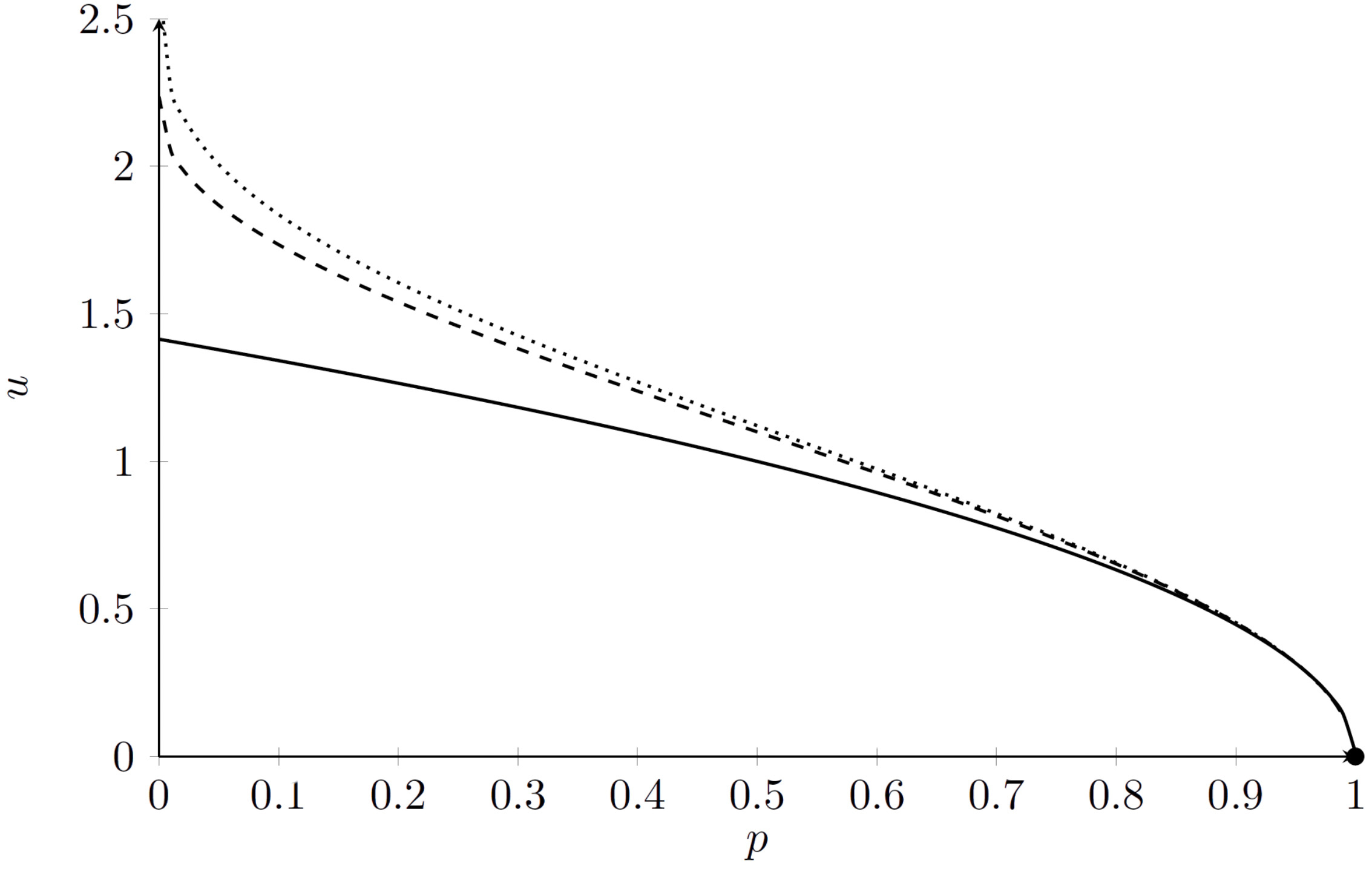
The Fig. 1 illustrates the relations between adimensional pressure and velocity according to BEIF (equation 17) and BECF (equation 22) for $n_f=3$ (monoatomic gas) and $n_f=5$ (diatomic gas without vibration), in the range $0\le p\le 1$.

Figure 1
Comparison of dimensionless velocity-pressure relationships for BEIF (equation 17, solid line), BECF (equation 22) with $n_f=3$ (dashed line), and $n_f=5$ (dotted line), in the range $0\le p\le 1$. The stagnation point at $\left(p=1,u=0\right)$ is marked with a black dot.

A complete comparison between BECF and BEIF must include the relationship between velocity and density. We rewrite BECF (equation 22) using the adiabatic relation (equation 19) as

(23) $$\frac{u^2}{2}+\left(1+\frac{n_f}{2}\right)d^{\frac{2}{n_f}}=\left(1+\frac{n_f}{2}\right).$$

The condition $n_f=0$ in equation 23 results in a singularity in the exponent $2/n_f$. We can circumvent this problem by considering the limit $n_f\to 0$, which yields $d=1$. Although $d=1$ describes the uniform fluid density of BEIF, substituting $n_f\to 0$ and $d=1$ into equation 23 results in $u=0$, which does not correspond to BEIF (equation 17). Thus, BEIF is not a particular case of BECF (equation 23) when the adiabatic relation is imposed.

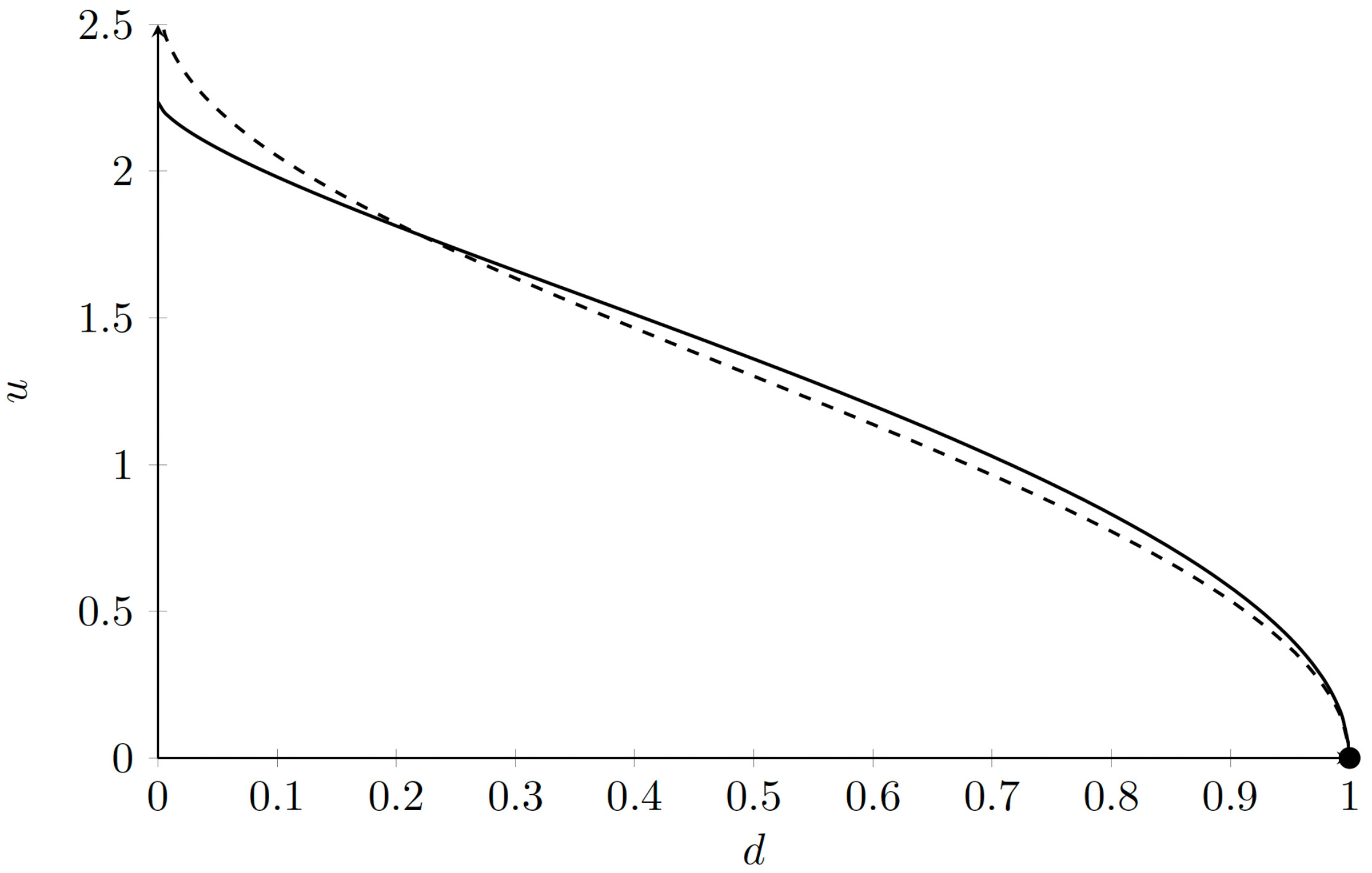
Analogously to Fig. 1, Fig. 2 shows the relationship between dimensionless density and velocity for BECF (equation 22) with $n_f=3$ (monatomic gas) and $n_f=5$ (diatomic gas without vibration), in the range $0\le p\le 1$. The pressure-velocity relationship for BEIF (equation 17) does not appear explicitly in Fig. 2 because BEIF maintains constant density ($d=1$).

Figure 2
Comparison of density-velocity relationships for BECF (equation 23) with $n_f=3$ (solid line) and $n_f=5$ (dashed line). For BEIF (equation 17), $d=1$. The stagnation point at $\left(d=1,u=0\right)$ is marked with a black dot.

7.1. Regime for low velocities

Figure 1 illustrates that the results for BEIF and BECF are similar at low velocities. In particular, Fig. 2 exhibits $d\approx 1$ (uniform fluid density) for low velocities. The agreement between BECF and BEIF at low velocities is consistent with the literature [⁴].

A superficial analysis suggests that equations 17 and 16 naturally explain the convergence of both equations at low velocities. If the thermal term is approximately uniform for low velocities ($n_{f}p/2d\approx n_f/2$), BECF (equation 16) becomes similar to the BEIF (equation 17).

In addition, we examine the implications of this assumption within the BECF directly. The approximation $n_{f}p/2d\approx n_f/2$ for BECF implies that $p/d\approx 1$. If this condition holds, equation 16 reduces to $u^2\approx 0$, a result which is demonstrably not equivalent to BEIF (equation 17).

It is unnecessary to prove that BECF converges to BEIF at low velocities, as this result is established in the literature [⁴]. In this work, we prove that BECF converges to BEIF to understand the reason for this convergence. The proof is as follows.

Equations 16 and 22 imply that

(24) $$\frac{p}{d}+\frac{n_f}{2}\frac{p}{d}=\left(\frac{n_f+2}{2}\right)p^{\frac{2}{n_f+2}}$$

We succeed by analyzing the low-velocity limit of BECF through the condition $u\underset{˜}{>}0$ in equation 22. In this regime, the dimensionless pressure $p$ approaches $1$ ($\left|p-1\right|\ll 1$). Writing the dimensionless pressure as $1+\left(p-1\right)$, the small deviation $p-1$ allows us to apply the binomial approximation ${\left(1+\delta \right)}^n\approx 1+n\delta$ to $p^{\frac{2}{n_f+2}}$. We obtain:

(25) $$p^{\frac{2}{n_f+2}}={\left(1+\left(p-1\right)\right)}^{\frac{2}{n_f+2}}\approx 1+\frac{2}{n_f+2}\left(p-1\right)=\frac{n_f+2p}{n_f+2}.$$

The above approximation (equation 25) in equation 24 implies that

(26) $$\frac{p}{d}+\frac{n_f}{2}\frac{p}{d}\approx p+\frac{n_f}{2}.$$

Replacing directly the approximation (equation 26) in BECF (equation 16), we obtain

(27) $$\frac{u^2}{2}+p+\frac{n_f}{2}=1+\frac{n_f}{2}.$$

equation 27 is equivalent to equation 17. However, the convergence of BECF to BEIF does not mean that $n_{f}p/2d\approx n_f/2$ in BECF (equation 16) at low velocities. Comparing equations 27 and 9, the dimensionless stagnation thermal term, $n_f/2$, behaves as a uniform dimensionless thermal density $E_{th}$.

Thus, the convergence from BECF (equation 16) to BEIF (equation 17) is related to the two sides of the approximation (equation 26): $p/d+n_{f}p/2d$ and $p+n_f/2$. When $u=0$, both BEIF (equation 17) and BECF (equations 22 and 23) have the same solution $p=d=1$, both sides of equation 26 equal $\left(n_f+2\right)/2$, and the approximation (equation 26) becomes an exact identity.

For low velocities, where $u\approx 0$ results in $p\approx 1$ and $d\approx 1$, the approximation (equation 26) remains valid. Even as $u$ increases further, leading to $p\not\approx 1$ and $d\not\approx 1$, the inequalities $p/d>p$ and $n_{f}p/2d<n_f/2$ can be expressed as $p/d=p+{\delta }_1$ (${\delta }_1>0$) and $n_{f}p/2d=n_f/2-{\delta }_2$ (${\delta }_2>0$). If ${\delta }_1\approx {\delta }_2$, the approximation (equation 26) remains valid. The approximation (equation 26), and the consequent convergence from BECF to BEIF, become invalid only when ${\delta }_1\not\approx {\delta }_2$ due to increasing $u$.

Tables 1 and 2 show that the BEIF (equation 17) and BECF (equation 22) solutions, for $n_f=3$ (Table 1) and $n_f=5$ (Table 2), converge as the dimensionless velocity $u$ approaches zero. Moreover, these tables demonstrate that BEIF-BECF convergence correlates with the proximity between $\frac{p}{d}+\frac{n_{f}p}{2d}$ and $p+\frac{n_f}{2}$. Conversely, their divergence grows with increasing $u$ and separation between $\frac{p}{d}+\frac{n_{f}p}{2d}$ and $p+\frac{n_f}{2}$.

Table 1
The first column represents the dimensionless velocity $u$. The second and third columns exhibit the dimensionless pressures $p$ for BEIF (equation 17) and BECF (equation 22) with $n_f=3$. The fourth column shows the dimensionless fluid density for BECF (equation 23) with $n_f=3$. The fifth and sixth columns contain the dimensionless quantities $p/d+n_{f}p/2d$ and $p+n_f/2$, whose proximity determines the convergence from BECF to BEIF. The seventh column represents the Mach number $M$.

$u$	$p$(BEIF)	$p$(BECF)	$d$(BECF)	$p/d+n_{f}p/2d$	$p+n_f/2$	$M$
0.0000	1.0000	1.0000	1.0000	2.5000	2.5000	0.0000
0.1000	0.9950	0.9950	0.9970	2.4950	2.4950	0.0775
0.2000	0.9800	0.9801	0.9880	2.4800	2.4801	0.1555
0.3000	0.9550	0.9556	0.9731	2.4550	2.4556	0.2345
0.4000	0.9200	0.9219	0.9524	2.4200	2.4219	0.3149
0.5000	0.8750	0.8796	0.9259	2.3750	2.3796	0.3974
0.6000	0.8200	0.8296	0.8940	2.3200	2.3296	0.4825
0.7000	0.7550	0.7727	0.8567	2.2550	2.2727	0.5709
0.8000	0.6800	0.7101	0.8143	2.1800	2.2101	0.6636
0.9000	0.5950	0.6429	0.7671	2.0950	2.1429	0.7615
1.0000	0.5000	0.5724	0.7155	2.0000	2.0724	0.8660
1.1000	0.3950	0.5002	0.6599	1.8950	2.0002	0.9787
1.2000	0.2800	0.4278	0.6008	1.7800	1.9278	1.1016
1.3000	0.1550	0.3566	0.5386	1.6550	1.8566	1.2376
1.4000	0.0200	0.2882	0.4741	1.5200	1.7882	1.3908

Table 2
Same columns as Table 1 but with $n_f=5$.

$u$	$p\left(BEIF\right)$	$p\left(BECF\right)$	$d\left(BECF\right)$	$p/d+n_{f}p/2d$	$p+n_f/2$	$M$
0.0	1.0000	1.0000	1.0000	3.5000	3.5000	0.0000
0.1	0.9950	0.9950	0.9964	3.4950	3.4950	0.0846
0.2	0.9800	0.9801	0.9858	3.4800	3.4801	0.1695
0.3	0.9550	0.9557	0.9682	3.4550	3.4557	0.2552
0.4	0.9200	0.9223	0.9438	3.4200	3.4223	0.3420
0.5	0.8750	0.8805	0.9131	3.3750	3.3805	0.4303
0.6	0.8200	0.8313	0.8763	3.3200	3.3313	0.5207
0.7	0.7550	0.7757	0.8341	3.2550	3.2757	0.6135
0.8	0.6800	0.7149	0.7869	3.1800	3.2149	0.7093
0.9	0.5950	0.6502	0.7353	3.0950	3.1502	0.8089
1.0	0.5000	0.5830	0.6802	3.0000	3.0830	0.9129
1.1	0.3950	0.5147	0.6222	2.8950	3.0147	1.0222
1.2	0.2800	0.4466	0.5623	2.7800	2.9466	1.1380
1.3	0.1550	0.3802	0.5012	2.6550	2.8802	1.2615
1.4	0.0200	0.3167	0.4399	2.5200	2.8167	1.3944

In Tables 1 and 2, the maximum dimensionless velocity is $u=1.4$, and we justify this restriction in the next subsection.

We include in Tables 1 and 2 the corresponding Mach number $M$ alongside the dimensionless velocity $u$ for ideal gases. The sound speed is given by $a=\sqrt{\gamma P/\rho }$ [⁴]. Using relation 6 with definitions 13, 14 and 15, we obtain:

(28) $$M=\frac{U}{a}=\frac{u\sqrt{\frac{P_0}{{\rho }_0}}}{\sqrt{\left(\frac{n_f+2}{n_f}\right)\frac{P}{\rho }}}=u\sqrt{\frac{n_{f}d}{\left(n_f+2\right)p}}$$

7.2. Regime for high velocities

The velocity in BECF (equation 16) cannot increase infinitely due to the constraint $p\ge 0$. The maximum achievable dimensionless velocity, $u_{max}$, is found by considering the limit $p\to 0$ in equation 16:

(29) $$u_{max}=\sqrt{2+n_f}.$$

Analogously to BECF, the maximum dimensionless velocity for BEIF is found through the limit $p\to 0$ in equation 17, yielding $u_{max}=\sqrt{2}$. Thus, the maximum velocity in expression 29 encompasses BEIF for $n_f=0$, although this case does not obey the adiabatic relation (equation 18).

Incompressible fluids can reach the maximum dimensionless velocity $u_{max}=\sqrt{2}$, because $p=0$ does not imply $T=0$ for incompressible fluids. However, for ideal gases, $p=0$ is equivalent to $T=0$, and the velocity cannot reach the maximum value. In this case, the velocity can approach the maximum value infinitely closely, but never reaches $u_{max}=\sqrt{2+n_f}$.

The fluid density behavior in BEIF and BECF differs fundamentally as the flow dimensionless velocity approaches its maximum value. For BEIF, the fluid density remains uniform and constant, even when $u=u_{max}=\sqrt{2}$. In contrast, for BECF, as $u\to \sqrt{2+n_f}$, the dimensionless pressure tends to zero ($p\to 0$), and the adiabatic relation (equation 18) implies that $d\to 0$, approaching a vacuum state.

Considering only the velocity-pressure relation, we may underestimate the difference between BEIF and BECF at high velocities. According to relation 29, the maximum dimensionless velocities for BEIF ($n_f=0$) and BECF with $n_f=3$ and $n_f=5$ are $\sqrt{2}\approx 1.4$, $\sqrt{5}\approx 2.2$, and $\sqrt{7}\approx 2.6$, respectively. Fig. 1 shows that the velocity-pressure relationships are relatively close over most of the range $0\le p\le 1$. However, Fig. 2 and Table 1 show that the velocity-density relationship changes dramatically with increasing dimensionless velocity: BEIF maintains $d=1$ for any velocity, while BECF decreases rapidly and approaches $d\to 0$ at maximum velocity.

We restrict the dimensionless velocity to $u\le 1.4$ in Tables 1 and 2 because this is approximately the maximum dimensionless velocity for BEIF, $u_{max}=\sqrt{2}\approx 1.4$. For $u>\sqrt{2}$, a comparison between BEIF and BECF is no longer meaningful.

8. Discussion

The main contributions of this work address three fundamental gaps in the fluid mechanics literature: demonstrating that BEIF can be written as a particular case of BECF; elucidating the physical meaning of BECF and its consequences; and rigorously exploring the differences between BEIF and BECF.

We identify three key obstacles to recognizing analogies between BEIF and BECF. First, the conventional forms of BEIF (equation 1) and BECF (equation 2) have different units, a problem resolved by the reformulation in equations 4 and 5. Second, in BECF (equation 2), the term $\gamma P/\left(\gamma -1\right)$ combines two physically distinct quantities: the thermal term, $n_{f}P/2\rho$, and the pressure term, $P/\rho$. Third, in BEIF (equation 4), the thermal term is implicit, as it is uniform and constant under the incompressibility assumption.

While the enthalpy and energy interpretations are successfully generalized from BEIF to BECF, we demonstrate that the conventional microscopic interpretation fails when applied to BECF. Consequently, we corroborate the findings of works that reject this conventional interpretation of Bernoulli’s equation at the particle level [⁸, ¹²].

This isotropic microscopic interpretation preserves the two key features from the general kinetic theory of fluids [¹⁴] cited in the Introduction: (1) the isotropy of the squared speed distribution for random particle motion, and (2) the necessity of including the role of intermolecular interactions.

As indicated in the Introduction, the literature suggests that BECF converges to BEIF for low velocities because an ideal gas behaves similarly to an incompressible fluid due to small fluid density variations [⁴]. In contrast, we demonstrate that the convergence of BECF to BEIF depends on a complex and counterintuitive relationship between velocity, pressure, and fluid density, which is precisely expressed by the approximation in equation 26.

This work opens up possibilities for introductory Fluid Mechanics courses. Instructors can present the BEIF and BECF as examples of mass, energy, and enthalpy transport. Furthermore, students can explore the concept of enthalpy beyond the standard example of isobaric transformations in ideal gases at rest. The isotropic interpretation of the BEIF and BECF at the molecular level illustrates the role of interparticle interactions in the fluid dynamics of incompressible and compressible flows, without resorting to the complex details of kinetic theory.

We suggest a specific didactic approach for introducing the BECF in the present work. Typically, the BECF in the form of equation 2 is presented as an analog of the BEIF for gases, converging to the BEIF itself for low velocities [², ⁴]. Here, we propose to formulate the BECF in equation 5 as the BEIF (equation 4) with additional thermal terms $n_{f}P/2\rho$ and $n_f{P}_0/2\rho$. However, it is essential that Fluid Mechanics courses emphasize the implicit difference between the matter densities in the BEIF (equation 4) and the BECF (equation 5). In this way, everything students learn from the BEIF can be extended to the BECF, provided they take into account the additional thermal term and the corresponding variations in matter density.

Courses may also connect the thermal term $n_{f}P/2\rho$ to the thermal energy in the kinetic theory of gases. While in the BEIF the pressure gradient produces only a kinetic energy variation, in the BECF the thermal energy accounts for part of the energy variation. Consequently, the same velocity change, associated with kinetic energy variation, produces a smaller pressure change in the BECF (see Tables 1 and 2). Moreover, the larger the number of degrees of freedom available for energy storage in the molecules, $n_f$, the greater the thermal energy per unit mass, $n_{f}P/2\rho$. Thus, increasing $n_f$ corresponds to an increase in thermal energy, leading to a more attenuated pressure variation with velocity (see Tables 1 and 2).

9. Conclusion

We conclude that both Bernoulli’s equations for incompressible and compressible fluids can be understood as describing the conservation of the sum of kinetic energy per unit mass, thermal energy per unit mass, and pressure per fluid density along each streamline. However, unlike compressible fluids, in incompressible fluids the thermal energy per unit mass is uniform, and this becomes implicit in the Bernoulli’s equation for incompressible flow.

Analogously to Bernoulli’s equation for incompressible flow, the version for compressible fluids can be interpreted as conservation of energy or enthalpy per unit mass. Furthermore, we can interpret that microscopic kinetic energy is present in both incompressible and compressible fluids, but the balance between macroscopic and microscopic kinetic energies occurs only in Bernoulli’s equation for compressible flow; for incompressible fluids, the intermolecular interactions balance the microscopic kinetic energy, preventing its conversion into other macroscopic energy forms.

The relation between velocity, pressure, and fluid density is radically different in each version of Bernoulli’s equation. The convergence from Bernoulli’s equation for compressible flow to its incompressible equivalent depends on a complex and counterintuitive relation between velocity, pressure, and fluid density. Both Bernoulli’s equations predict a maximum velocity reached at zero pressure. However, only incompressible fluids can actually attain this maximum velocity, while compressible fluids exhibit coupled behavior where density and pressure approach zero simultaneously.

Acknowledgments

The authors would like to acknowledge the AI assistant DeepSeek (DeepSeek Chat) for linguistic polishing and grammatical review of the manuscript. It is important to note that the conceptual framework, mathematical derivations, and scientific conclusions remain entirely the authors’ original work. GAO has a post doctoral fellowship from Universidade de São Paulo, C2PO 1-2025.

Data Availability

The entire dataset supporting the results of this study was published in the article itself.

References

• ^[1] P. Fife, A Gentle Introduction to the Physics and Mathematics of Incompressible Flow Course Notes (Published by the author, 2000). Available in: https://www.math.utah.edu/~fogelson/6750_f09/paulfife_fluidnotes2000.pdf
  » https://www.math.utah.edu/~fogelson/6750_f09/paulfife_fluidnotes2000.pdf
• ^[2] J.M. McDonough, Lectures in Elementary Fluid Dynamics: Physics, Mathematics and Applications (University of Kentucky, Lexington, 2009).
• ^[3] J. Braithwaite, An Introduction to Hydrodynamics (Published by the author, 2011). Available in: http://elibrary.bsu.edu.az/files/books_400/N_224.pdf
  » http://elibrary.bsu.edu.az/files/books_400/N_224.pdf
• ^[4] Y. Nakayama and R.F. Boucher, Introduction to Fluid Mechanics (Butterworth-Heinemann, London, 1999).
• ^[5] G.A. Van Lear Jr., Am. J. Phys. 2, 99 (1934).
• ^[6] E.H. Kennard, Science 62, 243 (1925).
• ^[7] G.A. Lindsay, Am. J. Phys. 20, 86 (1952).
• ^[8] R.P. Bauman and R. Schwaneberg, Phys. Teach. 32, 478 (1994).
• ^[9] L.S.F. Santos, Rev. Bras. Ensino Fís. 46, e20230253 (2024).
• ^[10] K. Misaiko and J. Vesenka, in: Anais do Physics Education Research Conference (Portland, 2013).
• ^[11] F. Glover, Am. J. Phys. 36, 811 (1968).
• ^[12] L.S.F. Santos, Eur. J. Phys. 39, 035102 (2018).
• ^[13]C.A. Crummer, arXiv:nlin/0507032 (2005).
• ^[14] D. Tong, https://www.damtp.cam.ac.uk/user/tong/kintheory/kintheory.pdf (2012).
  » https://www.damtp.cam.ac.uk/user/tong/kintheory/kintheory.pdf
• ^[15] T.I. Gombosi, Gaskinetic Theory (Cambridge University Press, Cambridge, 1994).
• ^[16] A.S. Yurchenko and S.A. Yurchenko, Int. J. Sci. Technol. Res. 9, 430 (2020).

• 1
  The Mach number $M$ is defined as the ratio of the fluid velocity $U$ to the local speed of sound $a$, $M=U/a$. For example, when the fluid velocity is half the speed of sound ($U=0.5a$), $M=0.5$.
• 2
  Ideal gas model assumes particles interact only through elastic collisions, while real gases exhibit intermolecular attractions and repulsions between molecules. Above the critical temperature, real gases behave more closely to ideal gases, making the model highly useful.

Edited by

• Editor-in-Chief:
  Marcello Ferreira https://orcid.org/0000-0003-4945-3169

Publication Dates

• Publication in this collection
  20 Mar 2026
• Date of issue
  2026

History

• Received
  18 Nov 2025
• Reviewed
  30 Jan 2026
• Accepted
  20 Feb 2026